The Split Delivery Vehicle Routing Problem with Three-Dimensional Loading and Time Windows Constraints

Abstract

Besides routing and packing plans, synthetically considering the requirements of customers about service time is absolutely necessary. An order split delivery plan can not only better satisfy the service time requirements, but also improve the full-load rate of vehicles. The split delivery vehicle routing problem with three-dimensional loading constraints (3L-SDVRP) combines vehicle routing and three-dimensional loading with additional packing constraints. In the 3L-SDVRP splitting deliveries of customers is basically possible, i.e., a customer can be visited in two or more tours. The vehicle routing problem with three-dimensional loading constraints that are based on the time window and considering split delivery of orders (3L-CVRPTWSDO) and its optimization algorithm are studied in this paper. We established mathematical model of the problem and designed the tabu search algorithm. Based on the examples used in Gendreau et al. (2006), examples was constructed to test our algorithm. The experimental results have expressed that, in the 3L-CVRP problem, the results of split delivery is better than those of non-split delivery, and it is easier to satisfy the time window constraints. The algorithm in this paper generates high quality solutions, it provides a effective method to solve the 3L-CVRPTWSDO problems.

1. Introduction

As the most important and basic activity in logistics, transportation will cause serious pollution to the environment. The specific performance is the traffic vehicle itself produces noise pollution, air pollution, waste oil pollution, traffic congestion, unreasonable logistics node layout aggravates waste gas, and noise pollution. The research of logistics distribution management is benefit to reduce the environmental pollution that is caused by such activities and implement the strategy of sustainable development. The routing problem of logistics delivery line is the core of logistics distribution management. Researchers are usually boiling down to its vehicle routing problem (Vehicle Routing Problem, VRP). Improper vehicle routing leads to high energy consumption and excessive carbon emissions. According to statistics [1], transportation accounted for 14% of global carbon emissions, and road transport represented almost one-third of these emissions. With the enhancement of people’s awareness of environmental protection, the concept of low carbon environmental protection, energy conservation, and emission reduction has become a new guiding ideology for vehicle routing research. Therefore, a better feasible solution to the vehicle routing problem is the key to realize low carbon. Chang and Morlok (2005) [2] first proposed the vehicle routing problem considering fuel consumption. Similar to some literature on how to develop green logistics, such as Peng et al. (2019) [3] and Zhang et al. (2020) [4], our research has a positive impact on transport sustainability.

In the actual distribution problem, the customer sometimes concentrates on the delivery time interval, and this time interval is usually called “time window”. The time window can be divided into hard time window and soft time window according to the severity of requirements or whether the corresponding price is allowed. In practical problems, we can limit the hard time window by setting the cost of time window deviation to infinity. From this, we can see that the hard window is actually a special case of the soft window type.

Traditional VRP can bring waste from using excessive vehicle to serve a small amount of customer. Customers’ needs are sometimes allowed to be split up and shipped in separate vehicles in order to reduce transportation costs and waste of resources. In this way, the loading capacity of the vehicle can be fully utilized and the driving cost of the vehicle can be reduced. Moshe Dror and Pierre Trudeau investigated the delivery of demand points that can be assigned among any number of vehicles and solved the computation-difficult split delivery vehicle routing problem (Split Delivery Vehicle Routing Problem, SDVRP) by using heuristic rules.

However, researches show that if only consider the customer’s service time window constraints and split orders, the result will often be that, even if the total volume of the loaded cargoes is smaller than the total volume of the vehicle, it still will not be able to load successfully because of the incorrect loading method and sequence. Aiming at this problem, Andreas Bortfeldt and Yi Junming (2018) [5] studied to expand SDVRP to the problem with three-dimensional (3D) loading constraints (3D-loading Split Delivery Vehicle Routing Problem, 3L-SDVRP) SDVRP. They propose a hybrid algorithm to solve this problem. This algorithm can generate high quality solutions with simple packaging plan structure in a short running time.

In this paper, we also refer to the research of Christos et al. [6] on “capacity vehicle routing problem with 3-D loading constraint (3L-CVRP)”. They believe that 3-D rectangular projects shapecustomer requirements. Transport problems should take into account the physical dimensions of the cargoes to be carried. They consider the various operational constraints that often occur in real-world situations to meet the various requirements of the customer. The purpose of this problem is also to design the route with the lowest cost, and the study of this problem also provides a reflection on how to reduce the waste of resources for the sustainable of this research.

This paper focuses on the problem that most organizations are required to adopt more sustainable methods in their logistics operations, and raises the vehicle routing problem with three-dimensional loading constraints based on the time window and considering split delivery of orders. We set up the corresponding delivery model, described and analyzed the characteristics of the problem. The proposed algorithm is analyzed by constructing a numerous practical test cases. Our algorithm reduces the total travel distance of transport vehicles in the same delivery process by improving the overall efficiency in the logistics process, which can reduce fuel consumption, save fuel costs, and reduce greenhouse gas emissions. This is consistent with the sustainable development strategy.

This paper is organized, as follows. In Section 2, the literature concerning the SDVRP problem and 3L-VRP problem is reviewed and existing approaches to the 3L-SDVRP problem are shortly described. In Section 3, we devise the loading scheme and delivery scheme of several vehicles that are involved in transportation activities in order to build a model. Section 4 designs the order splitting algorithm. Section 5 design the Deepest-Bottom-Leftfill algorithm. Section 6 studies the tabu search algorithm for route solution. In Section 7, numerical experiments are carried out and followed by the conclusion in Section 8.

2. Literature Review

In this section, the literature concerning the SDVRP problem and 3L-VRP problem is reviewed and existing approaches to the 3L-SDVRP problem are shortly described.

2.1. Vehicle Routing Problems with 3D Loading Constraints

The 3L-CVRP was introduced by Gendreau et al. (2006) [7] and motivated by a real furniture distribution decision in Italy. Besides geometrical constraints, exact-one-visit condition, and a weight constraint, they considered four loading constraints on orientation, fragility, vertical stability, and last-in-first-out policy (LIFO). The 3L-CVRP with these constraints is called here the Gendreau formulation of 3L-CVRP. Wang Lei (2009) [8] improve the method in Gendreau et al. (2006) [7] in his master thesis who replaces the tabu search algorithm of which 3D loading with local search. Its optimization results are almost the same with using tabu search and it effectively improves the program running efficiency. Xijun Li (2018) [9] use the distribution estimation algorithm. The problem is divided into three sub-questions: standard VRP vehicle distribution, SDR and customer cargo sub-carriage, 3D-bin loading.

Other features are also considered, such as time windows by Moura (2008) [10], who uses a multi-objective genetic algorithm. Additionally, time window combines with backhuals by Sebastian Rei (2018) [11] who uses a two-layer heuristic algorithm, its outer layer tabu search provides the routing plan, and the inner layer local search provides the packing plan.

2.2. Vehicle Routing Problem with Split Deliveries

There are two versions of the split delivery problem research.

The first version is the one in which demand can be divided in unlimited number of batches, but the total demand of all batches will be equal to the total demand of the customer. Dror and Trudeau (1989) [12] introduced the SDVRP problem, this paper examines a relaxed version of the generic vehicle routing problem. In this version, a delivery to a demand point can be split between any number of vehicles. Then they further refined the previous study in Dror and Trudeau (1990) [13]. Thereafter, the SDVRP problem further analyzed by Archetti et al. (2008) [14] and Archetti et al. (2011) [15]. They proposed a tabu search algorithm to solve such problems. Jin M. et al. (2008) [16] studied an integer programming algorithm for solving demand-splitable VRP.

The above split delivery problems are all based on the background that customer point demand can be arbitrarily divided (i.e., split according to unit of measurement). Actually, a customer’s order sometimes packages more than one piece of cargoes, which cannot be separately transported. The cargoes in the same order must be transported the same vehicle, such as the transportation of boxed milk. The order size is the number of cartons of milk, not the weight or volume of milk.

Therefore, in the second version, number of batches and the quantity of each batch is known in advance. Archetti, C et al. (2013) [17] show that the profit collected by allowing split deliveries may be as large as twice the profit collected under the constraint that each customer has to be served by one vehicle at most. The number of batches is known in advance in this paper. Archetti et al. (2015) [18] considered that, in actual operation, different cargo requires different handling tools, and cargoes of the same kind shall not be transproted separately. Besides, the tabu search algorithm is used by Fu Zhuo et al. (2017) [19] to solve the problem of capacity vehicle routing optimization with time window and order splitting, and the number of split orders per customer point is limited to five.

2.3. Approaches to 3L-VRPTW

The VRPTW problem was introduced by Solomon (1987) [20]. Moura (2008) [10] presented a multi-objective genetic algorithm for the 3L-VRPTW problem, while Moura and Oliveira (2009) [21] proposed different constructive heuristics for the same problem. Fu et al. (2008) [22] classified the main types of soft time Windows into six types and proposed an integrated tabu search algorithm that could solve various types of soft time Windows. Repoussis et al. (2009) [23] put forward an arc-guided evolutionary algorithm to solve the VRPTW problem. The method proposed by Bortfeldt and Homberger (2013) [24] consists of an evolutionary strategy and two tabu search procedures. A local search heuristic for the pallet packing VRPTW, which was considered as a variant of the 3L-VRPTW was discussed by Zachariades et al. (2016) [25]. The cargos of the customers are first packed on identical pallets that are then loaded onto vehicles. The practical application of Distributing fibred boards is studied by Pace et al. (2015) [26], and time windows and three-dimensional loading constraints was considerate in this paper.

2.4. Approaches to 3L-SDVRP

Moura and Oliveira (2009) [21] proposed two methods for the vehicle routing problem with time windows and 3D loading constraints. In their sequential method, a sequential candidate list (SCL) is defined and a candidate of SCL is composed of a client and a single box type of his demand. When none of the remaining candidates in the SCL can feasibly be assigned to the current vehicle, a new, empty vehicle is opened; thus, a candidate with the same client and a different box type might be assigned to a different vehicle. Ceschia et al. (2013) [27] deal with three problems: first, the 3L-CVRP in Gendreau formulation; second, an extended 3L-CVRP with difficult packing constraints (load bearing strength, robust stability, and reachability); and, third, a 3L-SDVRP with same packing constraints as in the second one. Ceschia tackle all three problems by a single-staged local search approach. Good results are achieved for well-known benchmark instances for the 3L-CVRP. To test their heuristic, they use 13 instances derived from practice and with limited vehicle fleet. The local search approach does not reach feasible solutions for all instances of the extended 3L-CVRP. In case of their 3L-SDVRP feasible solutions are provided, i.e., split delivery helped to achieve the missing feasible solutions. However, the results with split delivery are worse than those without split delivery, which contrasts with the classical SDVRP. Furthermore, relatively long running times of up to 10,000 s are reported. Li, Yuan et al. (2018) [9] propose a novel data-driven three-layer search algorithm to solve the 3L-SDVRP. They minimize the number of used vehicles with first and the total travel distance with second priority. Additionally, Li et al. add a packing material constraint and other process constraints for their industrial scenario in which an average delivery order contains more than 300 boxes to be distributed across the Pearl River Delta region. Yi and Bortfeldt (2018) [5] address the 3L-SDVRP with the same packing constraints as the 3L-CVRP in Gendreau formulation. Only inevitable splits are allowed, i.e., serving a customer in two or more routes is only permitted if not all boxes can be packed into a single loading space. A hybrid heuristic is developed that can be considered as a preliminary variant of the algorithm presented here. They further studied the above problem in Andreas Bortfeldt and Junmin Yi (2019) [28]. According to the actual situation, order splitting problem can also be divided into SDVRP-f (forced split) and SDVRP-o (optional split) two ways.

Splitting each customer’s order can avoid the situation that a customer’s cargoes cannot be loaded into one vehicle and the constraints are not satisfied, so more feasible packing schemes can be obtained. For the three-dimensional loading and vehicle routing combination optimization problem, splitting the customer’s demand according to the known order batch and quantity can increase the flexibility of packing and obtain the higher quality solution of the problem interest. On the other words, splitting the order by this way in which number of batches and quantity is known can avoid separating the cargoes which must be packaged delivery.

At present, there are fewer widely cited papers regarding the 3L-CVRPHTWSDO problem, so it can be said that there is a blank in the research of the problem.

3. Model Development

In the vehicle routing problem with three-dimensional loading constraints based on the time window and considering split delivery of orders, to achieve the best loading and delivery scheme within the loading capacity of the vehicle from the view of distribution center side, we devise the loading plan and delivery route of several vehicles that are involved in transportation activities. On the premise of the time window limit (the cargoes must reach the customer point after the earliest arrival time but before the latest arrival time), we split the customer’s order that can be delivered by several vehicles when the demand of a customer point is greater than the remaining loading capacity of the vehicle. The optimization objective of the problem is to determine a reasonable transportation route and three-dimensional loading plan in order to minimize the number of vehicles usage and the distance of vehicles under the condition that the vehicle loading capacity limit and time window limit. The first optimization objective is to minimize the use of vehicles and the second optimization objective is to minimize the vehicle travel distance.

Model Building

There are K customers and one depot (if variable’s $i=0$ represent depot’s variable in the following description). Each customer point’s $C_i({\alpha }_i,{\beta }_i)$ cargo demand is $I_i=I_i^1+I_i^2+\cdots +I_i^M(i=1,2,\cdots ,K)$. There are P vehicles coming to serve customers one-by-one, and finally return back to the depot. Each customer point’s demand can be served by several vehicle, but all demands $I_i$ must be satisfied after the configured earliest arrival time $A_i$ and before the latest arrival time $B_i$. Dimensions of these cargoes are known. Each $I_i^m$ involve each cargo’s length $l_i^m$, wide $w_i^m$, high $h_i^m$, and volume $v_i^m$ attributes. $Q_i$ is the vehicle’s capacity. There are four attributes (length $L_i$, wide $W_i$, high $H_i$, and volume $V_i$) for each vehicle’s $Q_i$.

Define other operational variables, as follows:

$b_{ij}$ is the travel distance from customer point i to customer point j:

$$b_{ij}=\sqrt{{\left({\alpha }_i-{\alpha }_j\right)}^2+{\left({\beta }_i-{\beta }_j\right)}^2}(i=1,2,\cdots K,j=1,2,\cdots K)$$

$\overline{t}$ is the unit time of vehicle pass through unit distance, $t_{ij}$ is the travel time from customer point i to customer point j:

$$t_{ij}=b_{ij}\overline{t}$$

$t_i$ is the time of reaching the customer point i. $t_{i_s}$ is the service time of customer point i. If customer point i and customer point j are on the same route, and service customer point j immediately after service customer point i, then:

$$t_j=t_i+t_{i_s}+t_{ij}$$

$Y_i^p$ means the cargoes that the vehicle p delivered to the customer point i. $X_{ij}^p$ and $h_{i_m}^p$ is the binary variable.

$$X_{ij}^p=\left\{\begin{array}{cc}1\hfill & \mathrm{Vehicle}\mathrm{P}\mathrm{travel}\mathrm{from}i\mathrm{to}j\hfill \\ 0\hfill & \mathrm{Otherwise}\hfill \end{array}\right.$$

$$h_{i_m}^p=\left\{\begin{array}{cc}1\hfill & \mathrm{Vehicle}P\mathrm{delivers}\mathrm{the}\mathrm{cargo}m\mathrm{to}\mathrm{custom}i\hfill \\ 0\hfill & \mathrm{Otherwise}\hfill \end{array}\right.$$

In three-dimensional loading plan, the assembly sequence is constructed in three directions on the number axis of the cartesian coordinate system in space, so that the newly added boxes are always located outside the packed boxes in each assembly sequence (away from the origin). In order to describe the relative position between the cargo and cargo or cargo and carriage. The position coordinates of the cargo $I_i^m$ at the far left, bottom and inside of the carriage are $x_i^m$, $y_i^m$ and $z_i^m$, relative position is $righ{t}_{mn}$, $fron{t}_{mn}$ and $to{p}_{mn}$.

$$righ{t}_{mn}=\left\{\begin{array}{cc}1\hfill & \mathrm{If}\mathrm{cargo}m\mathrm{is}\mathrm{on}\mathrm{the}\mathrm{right}\mathrm{of}\mathrm{cargo}n\hfill \\ 0\hfill & \mathrm{If}\mathrm{cargo}m\mathrm{is}\mathrm{on}\mathrm{the}\mathrm{left}\mathrm{of}\mathrm{cargo}n\hfill \end{array}\right.$$

$$fron{t}_{mn}=\left\{\begin{array}{cc}1\hfill & \mathrm{If}\mathrm{cargo}m\mathrm{is}\mathrm{in}\mathrm{front}\mathrm{of}\mathrm{cargo}n\hfill \\ 0\hfill & \mathrm{If}\mathrm{cargo}m\mathrm{is}\mathrm{behind}\mathrm{cargo}n\hfill \end{array}\right.$$

$$to{p}_{mn}=\left\{\begin{array}{cc}1\hfill & \mathrm{If}\mathrm{cargo}m\mathrm{is}\mathrm{above}\mathrm{cargo}n\hfill \\ 0\hfill & \mathrm{If}\mathrm{cargo}m\mathrm{is}\mathrm{below}\mathrm{cargo}n\hfill \end{array}\right.$$

The mathematical model can be described as

$$minP$$

(1)

$$minZ=\sum _{i=0}^K\sum _{j=0}^K\sum _{p=1}^P{b}_{ij}{X}_{ij}^p$$

(2)

$$\sum _{i=0}^K{Y}_i^p\le Q_i,p=1,2,\cdots ,P$$

(3)

$$\sum _{p=1}^P\sum _{i=1}^K{X}_{ij}^p\ge 1,j=1,2,\cdots ,K$$

(4)

$$\sum _{p=1}^P{Y}_i^p=I_i,i=1,2,\cdots ,K$$

(5)

$$A_i\le max{t}_i\le B_i,i=1,2\cdots ,K$$

(6)

$$\sum _{i=1}^{K}X{}_{ih}^p=\sum _{j=1}^K{X}_{hj}^p,h=1,2,\cdots K;p=1,2,\cdots ,P$$

(7)

$$Y_i^p=h_{i^1}^p{I}_i^1+h_{i^2}^p{I}_i^2+\cdots +h_{i^m}^p{I}_i^m,i=1,2,\cdots ,K;p=1,2,\cdots ,P$$

(8)

$$f=min(V_i-\sum _{m=1}^M{v}_i^m),i=1,2,\cdots ,K$$

(9)

$$0\le x_i^m\le W-w_i^m,x_i^m+(1-righ{t}_{mn})M\ge x_i^n+w_i^n$$

(10)

$$0\le y_i^m\le H-h_i^m,y_i^m+(1-to{p}_{mn})M\ge y_i^n+h_i^n$$

(11)

$$0\le z_i^m\le L-l_i^m,z_i^m+(1-fron{t}_{mn})M\ge z_i^n+l_i^n$$

(12)

$$fron{t}_{mn}+righ{t}_{mn}+to{p}_{mn}+fron{t}_{nm}+righ{t}_{nm}+to{p}_{nm}=1$$

(13)

In the above model:

• Formula (1) is the first optimization objective, minimize vehicle usage P.
• Formula (2) is the second optimization objective, minimize vehicle travel distance.
• Formula (3) is the vehicle loading capacity limit.
• Formulas (4) and (5) indicate that each customer point is accessed at least once, and the demand should be met.
• Formula (6) indicates that the vehicle must reach the customer point after the earlist arrival time but before the latest arrival time.
• Formula (7) indicates the conservation of flow, the number of vehicles entering a customer point is equal to the number of vehicles leaving the customer point.
• Formula (8) indicates that the requirements i the customer point can be split, but each order is not detachable.
• Formula (9) indicates the volume constraints of each vehicle.
• Formulas (10)–(12) indicates the cargoes are loaded by deep-bottom-leftfill method.
• Formula (13) indicates the loading position’s consistency.

4. Order Splitting Algorithm

4.1. Purpose of Order Splitting

The purpose of order splitting is to reduce the number or the total travel distance of the vehicles by merging the routes.

In the description of the order splitting mode in this paper, the node 0 is the warehouse, the cargos are sent out from the warehouse. Vehicles return to the warehouse after completing the distribution task. The arc between node i and node j is expressed as arc $(i,j)$. The route between node i and node j is expressed as route $(i,k,j)$ (k is a node or the nodes between node i and node j). For example, route $(0,3,4)$ means a route between node 0 and node 4, the vehicles start at node 0, then goes through node 3, and finally ends up at node 4.

4.1.1. Reduction in Number of Vehicles

As shown, splitting the order at node 3. In the example shown in Figure 1, the route $(0,1,2,0)$ and arc $(0,3)$ are merged into route $(0,1,2,3,0)$. The route $(0,3,4,0)$ is merged with route $(0,5,0)$ into route $(0,3,4,5,0)$. The number of vehicles is reduced from three to two.

4.1.2. Reduction in Total Distance

As shown, splitting the order at node 3. In the example shown in Figure 2, the route $(0,1,2,0)$ and arc $(0,3)$ after order splitting are merged into route $(0,1,2,3,0)$. In this example, the total distance of arc $(2,3)$ and arc $(0,3)$ is less than the total distance of arc $(0,2)$ and arc $(0,3)$.

4.2. Order Splitting Mode

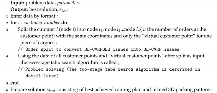
Set node i as “Split Customer”. Splitting the node i into node $i_1$, node $i_2$...node $i_N$ (N is the number of orders at the customer point). The nodes are called “virtual customer”. They have the same coordinates and only need one piece of cargos. “Split Customers” are always the last customer in the prior route and the first customer in the next route. In the subsequent tabu search algorithm, all “virtual customers” split from one point will be merged in the result due to the same coordinates of them.

In Algorithm 1, all of the customer points are treated as “Split Customers”. Thus, 3L-CVRPSDO problem has been transformed into 3L-CVRP problem. This makes it suitable for the two-stage tabu search algorithm of “route first, then load ”(the loading part of this paper uses the local search algorithm. The experimental results show that the optimization effect is almost the same as the tabu search).

Algorithm 1: Convert 3L-CVRPSDO to 3L-CVRP

4.3. Algorithm Overview

We transform 3L-CVRPSDO problem into 3L-CVRP problem. Subsequently, the two-stage tabu search algorithm will be called to solve the problem. The two-stage tabu search algorithm is described in detail in the next section.

5. Deepest-Bottom-Leftfill Algorithm

3L-CVRP was first proposed by Gendreau et al.(2006) [7], who considered geometrical constraints, exact-one-visit condition, weight constraints, and loading constraints in four facets, namely orientation, fragility, vertical stability, and last-in-first-out policy (LIFO). This is called Gendreau formula. In recent years, Gendreau formula has proposed a multitude of heuristic algorithms, such as deepest-bottom-leftfill for solving 3L-CVRP. We also use this method to complete our packing plan.

5.1. Deepest-Bottom-Leftfill Packing Mode

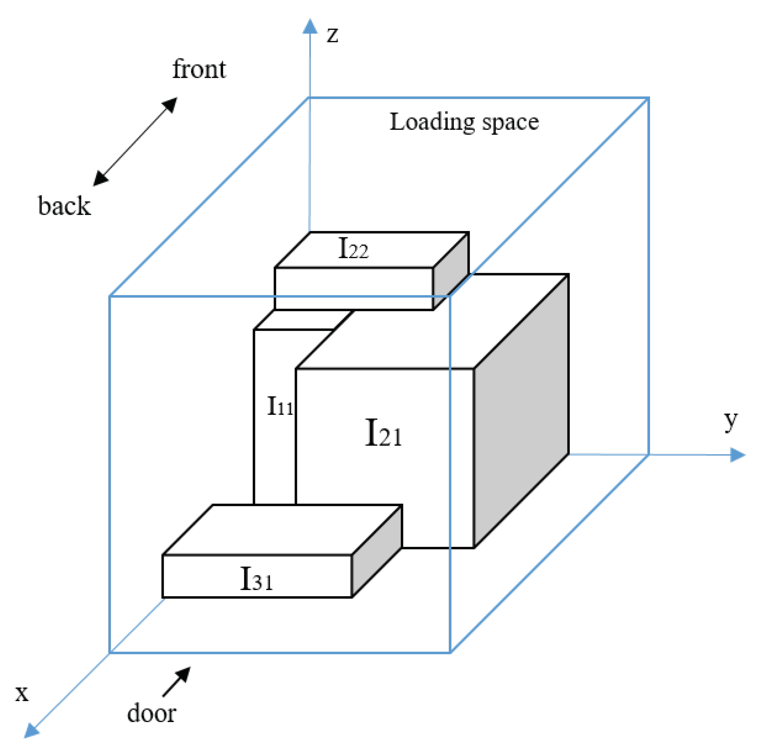
In the 3L-CVRP solution, there are n customers and a fixed distribution center (where the cargos are assembled). Each customer has a series of cargo boxes I of known size, which will be delivered from the distribution center to customer i$(i=1,...,n)$. Each series I has $m_i$ containers $I_k(k=1,...,m_i)$, and each cargo box $I_k$ has length $l_k$, width $w_k$, and height $h_k$.

The loading space of each car is placed into the first hexagram limit in cartesian coordinate system, and the length, width, and height of the loading space are respectively parallel to the X-axis, Y-axis and Z-axis of cartesian coordinate system. The position of each box $I_k$ in the loading space is given by the box angle coordinates $x_k$, $y_k$, and $z_k$, which are closest to the origin of the coordinate system.

If an assembly scheme satisfies the following three conditions, we consider it feasible.

• Each container placed is completely located in the loading space.
• Any two containers placed in the same loading space shall not overlap.
• Each container is parallel to the surface of the loading space.

As shown in the Figure 3.

In addition, there are the following load and weight constraints:

• Weight constraint: each cargo container $I_i$${}_k$ has weight $d{b}_i$${}_k$$(i=1,...,n;k=1,...,n)$ the sum of the weight of all the cargo boxes in each loading scheme shall be less than the maximum load weight of the loading space.
• LIFO constraint: the cargo boxes of customers who are delivered later in the distribution routing cannot be placed on the upper or front side of the cargo boxes of customers who are delivered first. This ensures that all containers for each customer can be taken out without the need to move another customer’s containers.
• Vertical direction constraint: the height direction of each cargo box is fixed, and it is not allowed to rotate arbitrarily.
• Vertical stability constraint: if a cargo box is not placed on the floor of the vehicle, its underside needs to be supported by other boxes.

5.2. Algorithm Overview

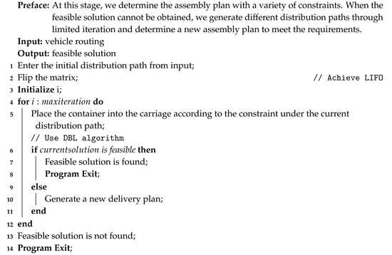
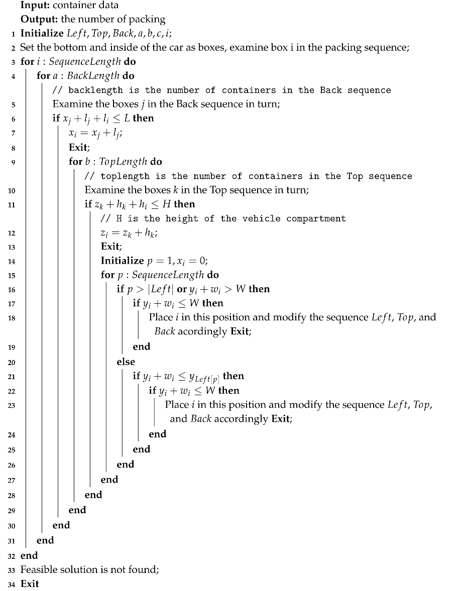
In this paper, local search and deepest-bottom-leftfill algorithm are used to generate the assembly scheme. We were given an assembly sequence Q, ordinal independent load each cargo tank. During loading, enumerated the x-coordinate first, place the cargo box in front of the loaded cargo box, then enumerate the z-coordinate, place the cargo box on the upper side of the loaded cargo box, and finally make it in the y direction to find the first feasible assembly position.

Now, we use the Algorithm 2 and the algorithm in Appendix A to calculate the assembly scheme. If the program returns a feasible solution, it indicates that we have found a feasible assembly scheme under the current distribution route.

Algorithm 2: Generate Feasible Assembly Plan

6. Tabu Search Algorithm for Route Solution

In the routing step, Gendreau et al. (2006) [7] adopt a saving algorithm (Clarke and Wright (1964) [29]) to find the initial solution, and then they used tabu search algorithm to seek a better solution, finally obtaining an optimal approximate solution through limited iterations. In the saving algorithm, they started a depot-customer-depot route for every customer and proceeded by amalgamating two routes into one until the vehicle number constraint was met. The merging rule is that the merged route must be totally feasible. In the tabu search algorithm, they explored neighbors of the initial solution by moving a customer from one route to another (operator called move-client).

Wang Lei (2009) [8] roughly followed this method and proposed a new algorithm, called two-stage tabu search algorithm, which start an initial solution and focus on searching a feasible solution in the first stage, continue to maintain the feasibility of the solution and search for the best solution in the second stage.

Through experiments, we found that the two-stage tabu search algorithm could be better to search a satisfactory solution by avoiding switching between feasible and infeasible solutions. Thus, we referred to Wang’s research to construct our tabu search algorithm.

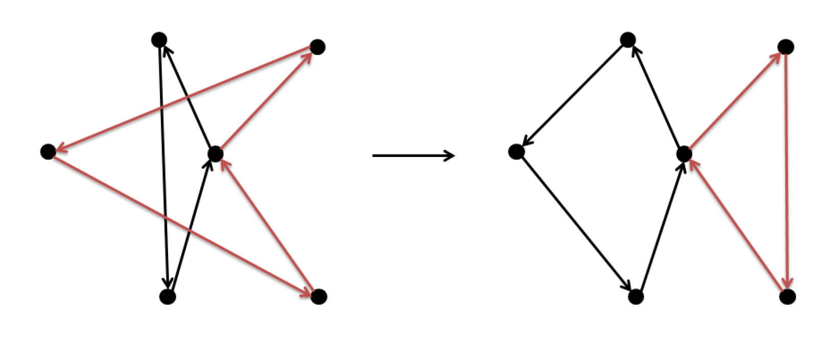
In the algorithm, we have four operators for moving solution:

1.

Cross-over:

We swap prefixes of two routes, and that will be described as Figure 4.

2.

Move-client:

This operator is the same as Gendreau’s. We randomly select a route to remove one of the customers and insert it into another route as Figure 5.

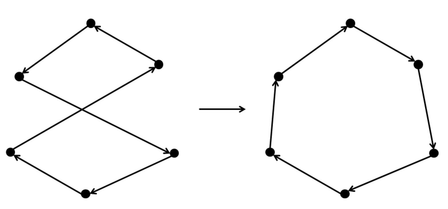
3.

2-opt:

This is a method frequently used in the traveling salesman problem (TSP). As we use this operator to move the solution, we will choose one route that has at least three customers to reverse a sub route of it. We can eliminate internal intersections of one route by this way as Figure 6.

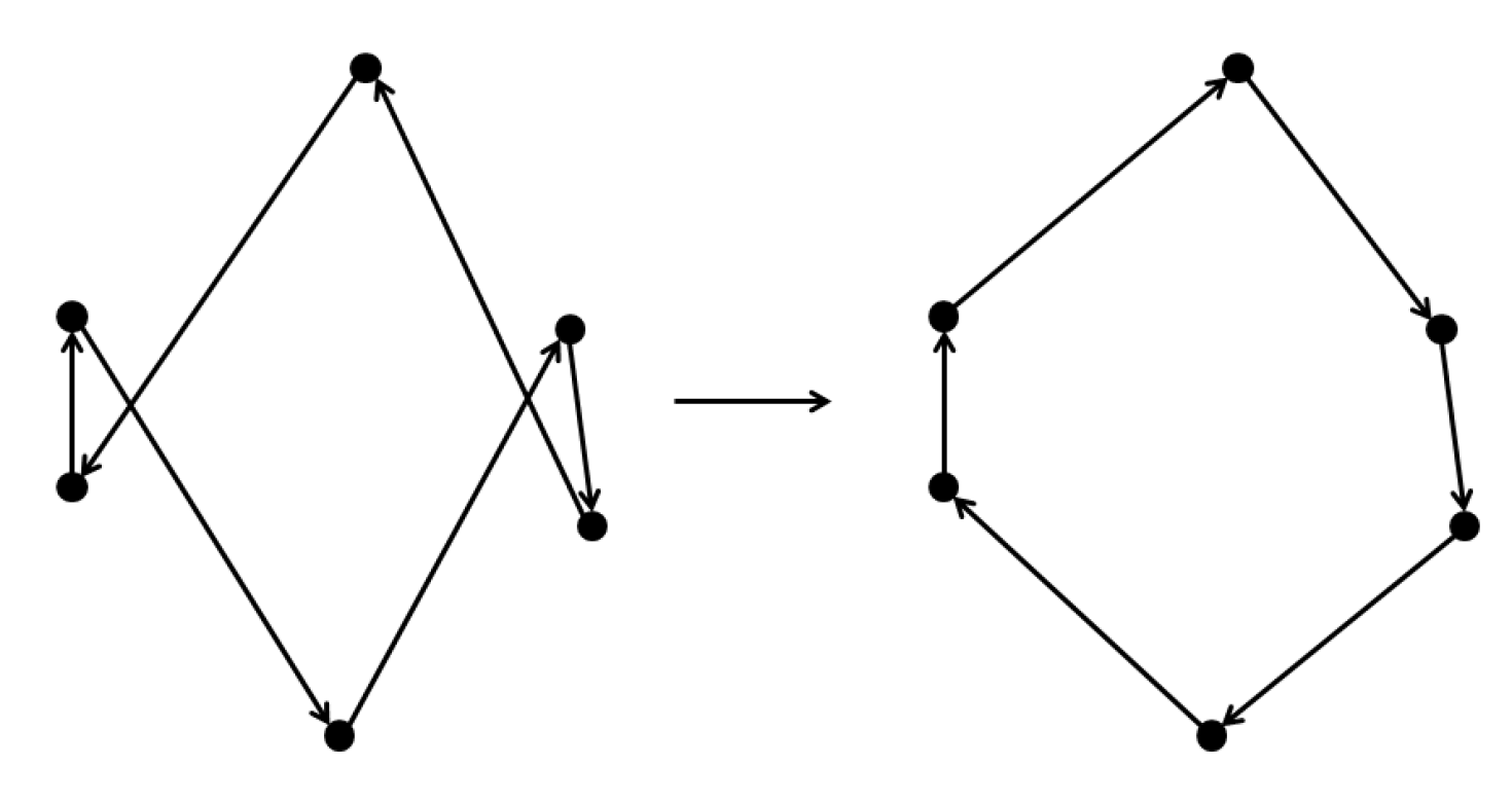
4.

2-swap:

We randomly select one route that contains more than three customers and swap two of the customers stochastically as Figure 7.

Tabu State

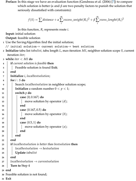
As shown in Algorithms 3 and 4, we set up two kinds of tabu list for different solution moves.

For operators (a), (c), (d), we build a $TabuClient\left[n\right]\left[n\right]$, where n is the number of customers, when a move involves two key customers i and j, we convert the status of the element $TabuClient\left[i\right]\left[j\right]$ from 0 to 1, which means that this move will be prohibited to produce a new neighbor solution in the next number of steps. For operator (b), we build a $TabuClient\left[n\right]\left[m\right]$ where n is the number of customers and m is the number of routes, when a move involves a key route j and a key customers i, we convert $TabuClient\left[i\right]\left[j\right]$ from 0 to 1.

Now, we obtained a feasible solution, then we will proceed to search further for an optimal solution.

For the above five algorithms, we integrate them to clarify the calling relationship of them. See Algorithm 5 for details.

Algorithm 3: Tabu Search Stage 1

Algorithm 4: Tabu Search Stage 2

Algorithm 5: Integration of Algorithms 1–5

1 Use algorithm 1 to convert 3L-CVRPSDO to 3L-CVRP and get a new input data model, $customernodes$

2 Use the Saving Algorithm to find the $initialsolution$

//$\phantom{(}$Call Algorithm 2 to check the feasibility, and the packing subprogram will call Algorithm 3 to load all the boxes$\phantom{(}$

3 Use tabu search stage 1 to search a $feasiblesolution$ through limited iterations, using initial solution from Saving Algorithm as the input1

//$\phantom{(}$In each iteration we will call the packing subprogram to check the feasibility of the solution$\phantom{(}$

4 Use tabu search stage 2 to search the $optimalsolution$, using the $feasiblesolution$ from Algorithm 4 as the input solution

//$\phantom{(}$In each iteration we will call the packing subprogram to check the feasibility of the solution$\phantom{(}$

5 Exit

7. Numerical Experiments

In this section, we firstly describe the setting value of the parameters, and then show the results of the experiment.

The examples we use are based on the first ten examples that used by Gendreau et al. (2006) [7] 3L-CVRP01–3L-CVRP10. The coordinates and requirements of the depot and customers, as well as the parameters of the box (length, width, weight, etc.) are exactly the same as these examples. About the time window constrains, we first test the approximate arrival time of each customer by experiments. Afterwards, add some random floating values to them to set the time window constrains.

We compare two optimization results with and without order splitting of the same example. The optimization effect of order splitting is verified.

The details of the examples we use can be found in the Appendix B of this paper. All of the experiments were run on a PC with a processor of Intel (r) core (tm)15-6300 hq cpu @ 2.30 ghz RAM 8 GB under Windows 10. The program of our algorithm was encoded with java “1.8.0_221”. Each example has been run five times.

7.1. Parameter Setting

Parameters $\alpha ,\beta ,\gamma$ are all related to $\overline{c}$, they need to be dynamically adjusted according to the example and the number of iterations. Some of the other parameters come from examples, others are determined through many experiments.

Table 1. Parameters of packing and routing.

Parameter	Meaning	Value
$\overline{c}$	Average of all edge weights	According to the example, according to the number of iterations state adjustment
$Node\_NUM$	Number of customer points	Based on the example
D	Vehicle load	Based on the example
L	Length of carriage	Based on the example
T	Single case service hours	3 (Customer hours Order boxes for the client ∗ T)
$\alpha$	Overweight Punishment Factor	20 $\overline{c}$/D
$\beta$	Extra long penalty factor	20 $\overline{c}$/L
$\gamma$	Time-out penalty factor	20 $\overline{c}$/T
$tabuLength$	Taboo length	30
$solutionSpace$	Solution space size	100
$maxIter1$	Number of first-stage iterations	5000
$maxIter2$	Number of second-stage iterations	10,000

shows how to set the value of the parameters.

This paper compares the quality of the feasible solution and the best solution to check whether the algorithm is improved. The approximate optimal is the key to the comparison. Hereinafter, the feasible solution in this paper represents the solution of the Tabu Search algorithm stage 1 in Algorithm 3, which can only reach a feasible solution not a best solution. The best solution represents the solution of the Tabu Search algorithm stage 2 in Algorithm 4, in which stage we can hold the feasibility of the solution of stage 1, and then search further to obtain an approximate optimal solution in all iterations. It shows the optimization effect of the algorithm.

The calculation formula of Solution Gap (Feasible and Best) is

$$\frac{(Feasible-Best)}{Feasible}$$

Additionally, that of Solution Gap (Best solutions of two algorithms) is

$$\frac{\left(\right(Best\left(left\right)-Best\left(right\right))}{Best\left(left\right)}$$

7.2. Comparison with Gendreau et al. (2006)

Before we take the time window constraint into account, we will compare our algorithm with the algorithm in Gendreau et al. (2006) that without split delivery to verify that if considering split delivery brings better optimization results, as shown in

Table 2. Statistical comparison of the data from the two algorithms.

Algorithm in Gendreau et al. (2006)				Algorithm in this Paper			Solution Gap
Node	Feasible	Best	Solution Gap (Feasible and Best)	Feasible	Best	Solution Gap (Feasible and Best)	Best Solutions of two Algorithms
1	356.35	309.02	13%	358.09	306.05	15%	1%
2	345.36	345.36	0%	357.68	322.81	10%	7%
3	465.69	465.69	0%	461.94	412.82	11%	11%
4	649.85	472.83	27%	575.38	466.84	19%	1%
5	490.63	490.63	0%	489.45	462.57	5%	6%
6	754.01	530.41	30%	601.50	511.24	15%	4%
7	1020.34	803.59	21%	866.02	803.59	7%	0%
8	897.22	785.69	12%	870.01	807.48	7%	−3%
9	1019.24	693.93	32%	769.93	657.68	15%	5%
10	917.93	835.98	9%	907.55	834.33	8%	0%
11	1049.05	1049.05	0%	1035.13	1035.13	0%	1%
12	837.13	691.21	17%	773.82	630.12	19%	9%
13	3005.20	2719.62	10%	3031.77	2710.84	11%	0%
14	1640.00	1551.82	5%	1670.68	1549.75	7%	0%
15	1767.82	1600.35	9%	1697.91	1551.91	9%	3%
16	811.31	719.08	11%	894.51	719.60	20%	0%
17	1011.61	917.11	9%	1099.93	892.31	19%	3%
18	1468.89	1370.42	7%	1341.51	1302.46	3%	5%
19	905.30	834.88	8%	911.23	847.37	7%	−1%
20	741.68	615.07	17%	746.10	591.03	21%	4%
21	1500.20	1240.24	17%	1314.99	1202.18	9%	3%
22	1555.22	1343.53	14%	1479.52	1288.68	13%	4%
23	1297.65	1210.17	7%	1869.24	1148.69	39%	5%
24	1432.17	1196.45	16%	1903.49	1202.57	37%	−1%
25	1841.05	1527.08	17%	2434.57	1584.30	35%	−4%
26	2645.45	1753.92	34%	2861.58	1838.50	36%	−5%
27	2132.53	1696.36	20%	1730.06	1595.17	8%	6%
Average Solution Gap	13%			15%			2%

and Figure 8.

As Table 2 shown, when compared to the algorithm in Gendreau et al. (2006) [7], we have an average optimization of 2%.

Betters results of the examples in the Gendreau et al. (2006) [7] also can be obtained after splitting. Experiments show that order splitting can bring obvious optimization effect.

7.3. Under the Time Window Constraint

In this section, we’re going to add the time window constrain(as shown in

Table 3. Summary of examples.

Numerical Example		Number of Nodes		Boxes Number		Number of Vehicles		Earliest Service Time		Latest Closing Time
1		15		32		4		10		150
2		15		26		5		0		110
3		20		37		4		0		200
4		20		36		6		0		140
5		21		45		6		0		110
6		21		40		6		0		100
7		22		46		6		0		180
8		22		43		6		0		110
9		25		50		8		5		170
10		29		62		8		5		200

) to test the performance of the algorithm with split delivery under time window constraints.

We are going to achieve the above goal by comparing the optimization effect of the same algorithm with and without split delivery.

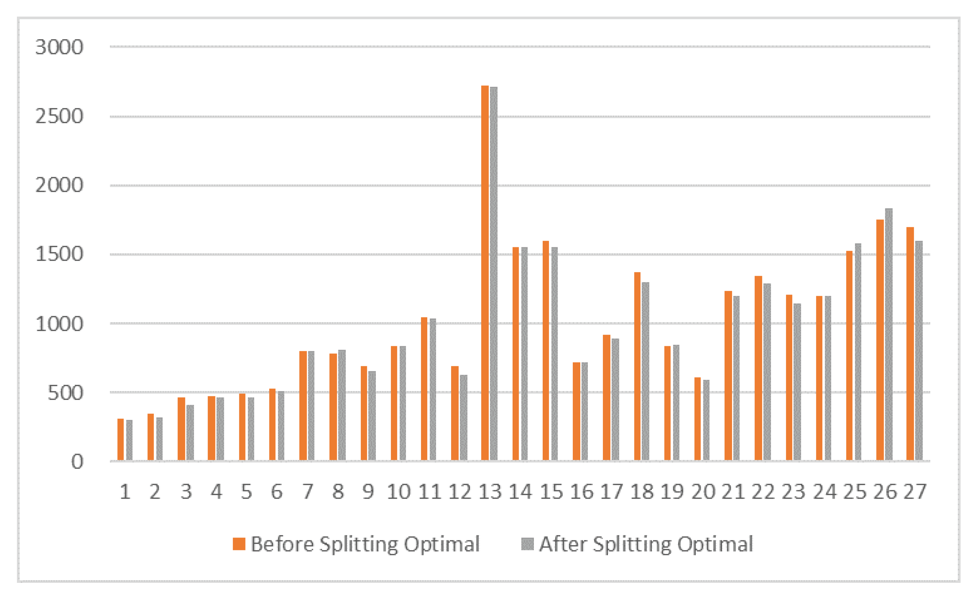
Before splitting represents the algorithm without split delivery process. After splitting represents the algorithm with split delivery process.

As

Table 4. Comparison of results before and after splitting.

	Before Splitting			After Splitting			Solution Gap
Node	Feasible	Best	Solution Gap (Feasibale and Best)	Feasible	Best	Solution Gap (Feasibale and Best)	Best Solutions of Two Algorithms
1	356.09	351.86	1.19%	361.15	307.66	14.81%	12.56%
2	353.91	353.91	0.00%	369.66	352.01	4.77%	0.54%
3	507.08	499.75	1.45%	520.52	512.42	1.56%	−2.54%
4	511.35	511.35	0.00%	528.05	528.05	0.00%	−3.27%
5	515.30	481.13	6.63%	594.88	455.49	23.43%	5.33%
6	771.64	514.02	33.39%	611.84	534.38	12.66%	−3.96%
7	1098.99	841.28	23.45%	857.71	850.63	0.83%	−1.11%
8	/	/	/	/	/	/	/
9	770.71	701.47	8.98%	674.45	583.08	13.55%	16.88%
10	/	/	/	1107.16	994.76	10.15%	/
Average Solution Gap	9%			9%			3%

shows, under the time window constraint, it is an average optimization of 3% in the case of split delivery.

Figure 9a,b and Table 4 show the statistical comparison of the examples before and after splitting by our algorithm. Because the time window constraints is not considered in Gendreau et al. (2006) [7], there might be no feasible solution of some examples. According to the experimental statistical results, our algorithm obtains the feasible solution and the best solution of eight sets of data before splitting, two sets of data have no feasible solution, the average running time of the algorithm before splitting is 76.7 s and the best solution reduces the average distance of 9.39%. When comparing with the data after splitting, it is not difficult to see that only one set of data cannot be solved after the order splitting is added, which shows that the algorithm with order splitting can analyze and calculate more cases. Additionally, these results also mean the algorithm with order splitting can satisfy the time window constrains more easily. The average running time of the algorithm with order splitting is 84.2 s. Its best solution compared with the feasible solution average distance decreased by 9.09%, which shows that the algorithm can get closer to the approximate optimal solution in fewer iterations. Order splitting greatly improves the efficiency and accuracy of the algorithm.

Split delivery reduced the average total travel distance by 3% under the window constraint (2% without the window constraint). It’s a reduction of three mile (two mile) per 100 miles. According to Reichmuth et al. (2013) [30], a hydrogen-fueled vehicle produces 0.2 kg CO2 per mile of vehicle travel distance. Accordingly, we can calculate the carbon emission by multiplying total distances covered by vehicles with the carbon emission conversion factor. This algorithm is equivalent to a reduction of carbon dioxide emission by 600 g (400 g) per 100 miles.

8. Conclusions

In this paper, we propose a new algorithm that includes two-layer tabu search algorithm and DBLF packing algorithm, it can be used to solve the 3D loading constrained vehicle routing problem that is based on hard time window that considers order splitting in practical application(3L-CVRPSTWSDO). This algorithm has a certain contribution to the research on vehicle routing and assembly at the same time, also focuses on the sustainable development, effective distribution can reduce automobile emissions of pollutants, the optimization results show that per car can reduce CO2 emissions by about 600 g per 100 miles, for the society, less carbon emissions can slow down the greenhouse effect and provide a better living environment.

The experimental results indicate that it is more efficient in comparison with the existing technical scheme, which is reflected in a 3% reduction in the total length of its distribution path. Moreover, it can solve multiple problems at the same time, in the first place it can solve the problem of resource waste that is caused by customer order can not be split when using traditional VRP algorithm, the other it can solve the problem the improper loading sequence and position of cargos when using SDVRP algorithm lead to even the waste of loading volume, the last but not least it can solve the problem of lack of authenticity and flexibility of distribution system caused by the VRP algorithm without time window. However, the new algorithm still has some limitations, the first is that there is only one pattern of order splitting. In addition, the ability of the algorithm to solve large-scale examples has not been verified. In the future, we can continue to adopt the machine learning-based method to improve this algorithm to obtain better results and make the algorithm sustainable. We expect this algorithm to fully demonstrate its capability.

References

- Wang, Y.; Zhou, Y.; Zhu, L.; Zhang, F.; Zhang, Y. Influencing Factors and Decoupling Elasticity of China’s Transportation Carbon Emissions. Energies 2018, 11, 1157. [Google Scholar] [CrossRef]
- Chang, D.J.; Morlok, E.K. Vehicle Speed Profiles to Minimize Work and Fuel Consumption. J. Transp. Eng. 2005, 131, 173–182. [Google Scholar] [CrossRef]
- Peng, B.; Zhang, Y.; Gajpal, Y.; Chen, X. A Memetic Algorithm for the Green Vehicle Routing Problem. Sustainability 2019, 11, 6055. [Google Scholar] [CrossRef]
- Zhang, W.; Gajpal, Y.; Appadoo, S.S.; Wei, Q. Multi-Depot Green Vehicle Routing Problem to Minimize Carbon Emissions. Sustainability 2020, 12, 3500. [Google Scholar] [CrossRef]
- Yi, J.; Bortfeldt, A. The Capacitated Vehicle Routing Problem with Three-Dimensional Loading Constraints and Split Delivery—A Case Study. Q. J. Oper. Res. 2018, 7, 351–356. [Google Scholar] [CrossRef]
- Tarantilis, C.D.; Zachariadis, E.E.; Kiranoudis, C.T. A Hybrid Metaheuristic Algorithm for the Integrated Vehicle Routing and Three-Dimensional Container-Loading Problem. IEEE Trans. Intell. Transp. Syst. 2009, 10, 255–271. [Google Scholar] [CrossRef]
- Gendreau, M.; Iori, M.; Laporte, G.; Martello, S. A Tabu Search Algorithm for a Routing and Container Loading Problem. Transp. Sci. 2006, 40, 342–350. [Google Scholar] [CrossRef]
- Lei, W. An Integrated Research for the Capacitated Vehicle Routing Problem with Container Loading. Ph.D. Thesis, Sun Yat-sen University, Guangzhou, China, 2009. [Google Scholar]
- Li, X.; Yuan, M.; Chen, D.; Yao, J.; Zeng, J. A Data-Driven Three-Layer Algorithm for Split Delivery Vehicle Routing Problem with 3D Container Loading Constraint. In Proceedings of the Knowledge Discovery and Data Mining, London, UK, 19–23 August 2018; pp. 528–536. [Google Scholar]
- Moura, A. A Multi-Objective Genetic Algorithm for the Vehicle Routing with Time Windows and Loading Problem. Intell. Decis. Support 2008. [Google Scholar] [CrossRef]
- Reil, S.; Bortfeldt, A.; MNch, L. Heuristics for Vehicle Routing Problems with Backhauls, Time Windows, and 3d Loading Constraints. Eur. J. Oper. Res. 2018, 266, 877–894. [Google Scholar] [CrossRef]
- Dror, M.; Trudeau, P. Savings by Split Delivery Routing. Transp. Sci. 1989, 23, 141–145. [Google Scholar] [CrossRef]
- Dror, M.; Trudeau, P. Split delivery routing. Nav. Res. Logist. 1990, 37, 383–402. [Google Scholar] [CrossRef]
- Archetti, C.; Savelsbergh, M.W.P.; Speranza, M.G. To split or not to split: That is the question. Transp. Res. Part E Logist. Transp. Review 2008, 44, 114–123. [Google Scholar] [CrossRef]
- Archetti, C.; Bianchessi, N.; Speranza, M.G. A Column Generation Approach for the Split Delivery Vehicle Routing Problem. Networks 2011, 58, 241–254. [Google Scholar] [CrossRef]
- Jin, M.; Liu, K.; Eksioglu, B. A column generation approach for the split delivery vehicle routing problem. Oper. Res. Lett. 2008, 36, 265–270. [Google Scholar] [CrossRef]
- Archetti, C.; Bianchessi, N.; Speranza, M.G.; Hertz, A. The split delivery capacitated team orienteering problem. Networks 2013, 63, 16–33. [Google Scholar] [CrossRef]
- Archetti, C.; Bianchessi, N.; Speranza, M.G. A branch-price-and-cut algorithm for the commodity constrained split delivery vehicle routing problem. Comput. Oper. Res. 2015, 64, 1–10. [Google Scholar] [CrossRef]
- Fu, Z.; Liu, W.; Qiu, M. The requirement of vehicle routing problem with soft time window and its tabu search algorithm. Chin. J. Manag. Sci. 2017, 025, 78–86. [Google Scholar]
- Solomon, M.M. Algorithms for the Vehicle Routing and Scheduling Problems with Time Window Constraints. Oper. Res. 1987, 35, 254–265. [Google Scholar] [CrossRef]
- Moura, A.; Oliveira, J.F. An integrated approach to the vehicle routing and container loading problems. OR Spectrum 2009, 31, 775–800. [Google Scholar] [CrossRef]
- Fu, Z.; Eglese, R.; Li, L.Y.O. A unified tabu search algorithm for vehicle routing problems with soft time windows. J. Oper. Res. Soc. 2008, 59, 663–673. [Google Scholar] [CrossRef]
- Repoussis, P.; Tarantilis, C.; Ioannou, G. Arc-Guided Evolutionary Algorithm for the Vehicle Routing Problem with Time Windows. IEEE Trans. Evol. Comput. 2009, 13, 624–647. [Google Scholar] [CrossRef]
- Bortfeldt, A.; Homberger, J. Packing first, routing second-a heuristic for the vehicle routing and loading problem. Comput. Oper. Res. 2013, 40, 873–885. [Google Scholar] [CrossRef]
- Zachariadis, E.E.; Tarantilis, C.D.; Kiranoudis, C.T. The Pallet-Packing Vehicle Routing Problem. Transp. Sci. 2016, 46, 341–358. [Google Scholar] [CrossRef]
- Pace, S.; Turky, A.; Moser, I.; Aleti, A. Distributing Fibre Boards: A Practical Application of the Heterogeneous Fleet Vehicle Routing Problem with Time Windows and Three-dimensional Loading Constraints. Procedia Comput. Sci. 2015, 51, 2257–2266. [Google Scholar] [CrossRef]
- Ceschia, S.; Schaerf, A.; Stutzle, T. Local search techniques for a routing-packing problem. Comput. Ind. Eng. 2013, 66, 1138–1149. [Google Scholar] [CrossRef]
- Bortfeldt, A.; Yi, J. The Split Delivery Vehicle Routing Problem with three-dimensional loading constraints. Eur. J. Oper. Res. 2019, 282, 545–558. [Google Scholar] [CrossRef]
- Clarke, G.; Wright, J.W. Scheduling of Vehicles from a Central Depot to a Number of Delivery Points. Oper. Res. 1964, 12, 568–581. [Google Scholar] [CrossRef]
- Reichmuth, D.S.; Lutz, A.E.; Manley, D.K.; Keller, J.O. Comparison of the technical potential for hydrogen, battery electric, and conventional light-duty vehicles to reduce greenhouse gas emissions and petroleum consumption in the United States. Int. J. Hydrog. Energy 2013, 38, 1200–1208. [Google Scholar] [CrossRef]
© 2020 by the authors. Licensee MDPI, Basel, Switzerland. This article is an open access article distributed under the terms and conditions of the Creative Commons Attribution (CC BY) license (http://creativecommons.org/licenses/by/4.0/).