Article

Solar Energy Prediction Model Based on Artificial Neural Networks and Open Data

by
Jose Manuel Barrera
1,2,*,
Alejandro Reina
1,2,
Alejandro Maté
1,2 and
Juan Carlos Trujillo
1,2
1
Department of Software and Computing Systems, University of Alicante, 03690 Alicante, Spain
2
Lucentia Lab, C/ Pintor Pérez Gil, N-16, 03540 Alicante, Spain
*
Author to whom correspondence should be addressed.
Sustainability 2020, 12(17), 6915; https://doi.org/10.3390/su12176915
Submission received: 4 July 2020 / Revised: 4 August 2020 / Accepted: 17 August 2020 / Published: 25 August 2020

Abstract

:
With climate change driving an increasingly stronger influence over governments and municipalities, sustainable development, and renewable energy are gaining traction across the globe. This is reflected within the EU 2030 agenda, that envisions a future where there is universal access to affordable, reliable and sustainable energy. One of the challenges to achieve this vision lies on the low reliability of certain renewable sources. While both particulars and public entities try to reach self-sufficiency through sustainable energy generation, it is unclear how much investment is needed to mitigate the unreliability introduced by natural factors such as varying wind speed and daylight across the year. In this sense, a tool that aids predicting the energy output of sustainable sources across the year for a particular location can aid greatly in making sustainable energy investments more efficient. In this paper, we make use of Open Data sources, Internet of Things (IoT) sensors and installations distributed across Europe to create such tool through the application of Artificial Neural Networks. We analyze how the different factors affect the prediction of energy production and how Open Data can be used to predict the expected output of sustainable sources. As a result, we facilitate users the necessary information to decide how much they wish to invest according to the desired energy output for their particular location. Compared to state-of-the-art proposals, our solution provides an abstraction layer focused on energy production, rather that radiation data, and can be trained and tailored for different locations using Open Data. Finally, our tests show that our proposal improves the accuracy of the forecasting, obtaining a lower mean squared error (MSE) of 0.040 compared to an MSE 0.055 from other proposals in the literature.

1. Introduction

Renewable energies have been gaining traction in the last decades. Non-polluting, and not limited by resources, these energies would be an ideal source of electricity for any activity, whether domestic or industrial, if it was not because of their unreliability. Indeed, renewable energies throughput varies significantly depending on the conditions and the characteristics of the place where they are located, which makes it difficult to estimate how much benefit in terms of power is going to be obtained from them.
One of the most relevant energies in recent years has been solar energy. Solar energy has a better-defined behavior than wind-based energies and harnesses considerable amounts of power from the sun in certain countries. As such, it is one of the most important renewable energies for a wide array of countries in south Europe, such as Spain, and other locations in the same longitude, such as Saudi Arabia [1] or India [2].
Solar energy can be broken down into two different kinds of energy: thermal solar energy, which converts solar radiation into thermal energy used for heating industrial processes, desalination plants, homes, or water purification plants, among others [3]; and photovoltaic solar energy, through which solar radiation is converted into electrical energy that can be transported for other uses than heating.
Despite this wide array of uses, photovoltaic energy presents varying performance from panel to panel, as shown in Figure 1. Combined with changing atmospheric conditions from the place where the panels are finally installed, it becomes challenging for customers to determine whether solar energy is a viable investment for them.
A potential solution for this problem would be to create a solar map, which contains the amount of solar energy received by each area annually. This approach has been applied successfully in certain Spanish towns [5]. Unfortunately, the cost involved in making these solar maps is considerable, which makes them widely unavailable. As a result, a large part of the potential self-producers of solar energy stop their investment, since they do not have the appropriate tools to estimate the technical-economic viability of the project.
Compared to existing approaches, in this paper, we propose a solution based on neural networks that helps to easily estimate the energy output of the solar panels installed in the target area while being significantly less costly than solar maps. Currently, a considerable part of the literature focuses on solar radiation forecasting rather than solar energy production prediction. This introduces additional uncertainty for users, since they only know how much energy their installation will receive, but not how much energy it will produce. Moreover, so far studies are built upon private data, limiting the applicability of the solutions proposed, due to the difficulty to find or build the necessary data to train and run the models. Taking this into account, the advantages that our approach presents are as follows:
  • It can be built from Open Data. Therefore, it only requires data that can be freely found available on the web, and anyone with technical knowledge can build their own tailored version.
  • It focuses on energy production, rather than solar radiation. Consequently, we are adding an abstraction layer that can answer higher-level questions. These questions range from analyzing the suitability of a specific place for a solar installation to its return on investment (ROI) from an economic point of view.
  • It provides solid accuracy results. The approach provides competitive results on the MSE (Mean Squared Error) and MAE (Mean Absolute Error) metrics that have been found in the literature.
Thus, our solution can be built and adapted for most areas around the world, providing a great substitute for locations where solar maps are not available. Therefore, thanks to our approach, the risk of installing new solar energy panels will be reduced and investments in new installations will be fostered.
The remainder of this paper is structured as follows. Section 2 presents the related work in solar energy models. Section 3 covers the aspects related to solar energy generation that must be taken into account for the neural network. Section 4 presents the structure of the different topologies and experiments carried out, and presents our solution for solar energy forecasting. Section 5 discusses the results and limitations of the approach, and finally, Section 6 describes the conclusions and sketches future works.

2. Related Work

In this section, we provide information about the state of the art literature in the research field and we point out the main advantages that our proposal can provide to the research community.
Many solar energy models have been proposed in the literature using different techniques and approaches. For instance, linear mathematical functions have been used on different project as in Algeria [6], with Satellite data [7], in sparse regions [8], or in Malaysia [9]. On the other hand, non-linear functions have been used for calculating daily diffuse solar radiation [10], irradiation models [11], and they have been combined with Ångstrom coefficients in quadratic models [12] and unrestricted methods [13]. If we focus on fuzzy logic approach, it has been used with meteorological parameters [14] and for short-term energy forecasting [15]. Finally, we can find genetic algorithms used in order to achieve the self-sustainability of a pump [16] and finally, the use of artificial neural networks (ANN).
Linear models present the advantages of being easily understandable, and their linearity makes them a suitable tool that will guarantee finding optimal weights to every component (and consequently, a quasi-optimal solution) if a linear relation exists. However, linear models usually present poor predictive performance, because the relationships that can be learned are so restricted that they usually oversimplify a complex reality. In addition, linear models are very sensitive to outliers (anomalies). Thus, outliers should be clearly identified and removed before applying the linear functions, which is not always an easy task.
Non-linear functions present the advantage of being capable of dealing with more complex relationships (since they are not constrained only to linear functions). However, because there are so many candidates, it can be necessary to conduct some research to determine which function provides the best fit for the data at hand. In turn, they require a significantly higher time investment than linear models.
Fuzzy logic models have the advantage that can deal properly with imprecise data thanks to their well-defined rule base. This capability provides more flexibility whereas other methods get compromised. Nevertheless, the disadvantages outnumber the advantages: the design of the rules can be very complex, it is necessary to have domain knowledge in order to deal properly with the problem presented, and defining precise values for creating the rule base can be difficult.
Genetic algorithms are a suitable tool when a quasi-optimal solution is needed. In addition, they manage noisy functions better than linear models. However, these algorithms require convergence, which may require a long time and a decent-sized population, making this approach very costly from a temporal point of view.
Finally, ANNs and their use in the field of solar energy deserve a separate section. ANNs exploit the use of graphic cards for boosting their computation speed [17]. This makes these systems optimal for prediction in multidimensional spaces, where their high cardinality makes it much more likely to find non-linear functions between different magnitudes or dimensions. Nevertheless, this ability to adapt to the distribution function presents the problem that it is very possible that the neural network largely overfits the training data, producing the effect called “overfitting” [18]. When this happens, the ANN “memorizes” the data received and loses its capability of prediction. This can create a false sense of accuracy in the model. To avoid this, a split of the data must be carried out between training models and test models (80%–20% or 90%–10% for different samples), with the aim of obtaining what would be the degree of accuracy of the model trained with completely unknown samples. Due to their suitability for multidimensional spaces, ANNs have been widely used in the solar energy field. A great variety of models have been presented, both for the construction of solar panels [19], and for the field of solar energy modeling in Nigeria [20], stand-alone installations [21], daily local energy radiation forecasting [22], residential stand-alone self-sustainability [23], solar power forecasting [24], 24-h-ahead energy production prediction [25], or global forecasting of energy prediction in Spain [26].
However, these approaches present some problems. On one hand, in [20], general aggregated values from solar radiation for a whole month were used in the forecasting. In contrast, our approach breaks down values from solar radiation (one for every 5 min) in order to allow our ANN to calculate the amount of energy generated even across very short ranges of time. On the other hand, references [21,22] have been used to forecast solar radiation, whereas in our approach we focus on solar power output prediction. In this way, we provide an abstraction layer to the customer, focused ROI of the installation. In [23], the authors focused on the ROI of the solar installation. However, this ANN was focused on a specific stand-alone installation, while our ANN aims to provide a general method that could be applied to almost any installation as long as their characteristics are provided. Finally, compared to the structure of the ANN in [24] and [25], our structure focuses on predicting the output of specific installations located in specific places, instead of general solar power forecast.
To better understand our model, in the next section we cover the factors that influence solar energy generation

3. Input Data for Solar Energy Prediction

In order to design an ANN for solar energy prediction, it is important to analyze the main factors that affect solar energy generation. These factors will have to be considered by the model as inputs, which will need to be adequately tailored for each particular situation we wish to predict. Therefore, in the following, we analyze these elements and how they affect solar energy production.
The first set of elements that has an influence on solar energy forecasting are solar components. These components provide the solar energy input to be processed and converted into electrical energy, such as with the excitation of electrons in a photovoltaic cell, generating energy from a renewable source. There are three solar components [27] that lead to energy production on a solar panel:
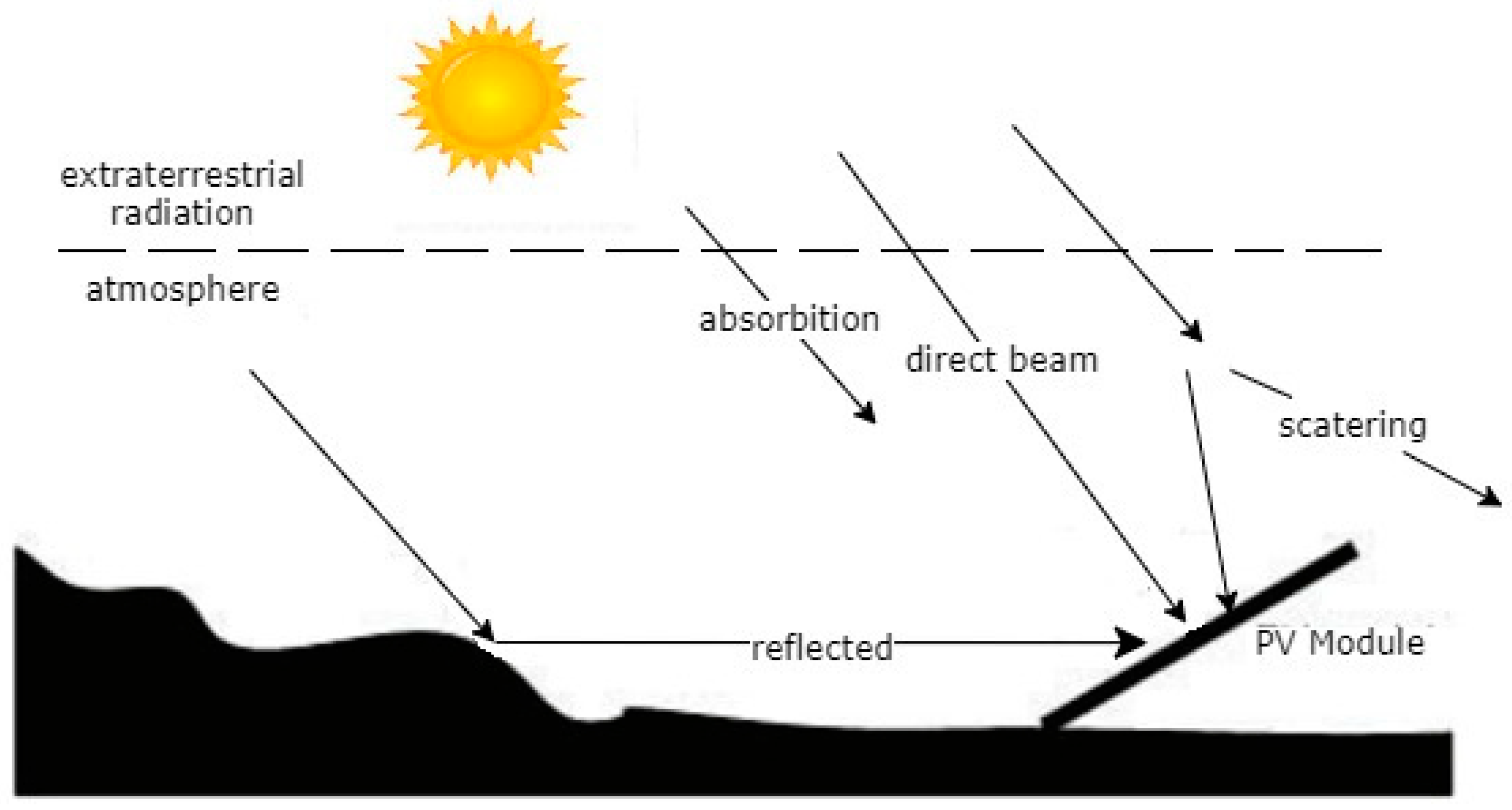
  • Direct radiation: Direct radiation is the component that is neither reflected nor scattered, reaching the directly the surface.
  • Diffuse radiation: Diffuse radiation is the component of the solar energy that is scattered by the atmosphere and reaches the surface.
  • Reflected radiation: Reflected radiation is the part of the radiation reflected by the surface or other elements and reaches the surface.
These three solar components can be combined (sum) into a Global Radiation value. However, this value does not take into account the angle at which solar rays reach solar panels, which alters the energy input received. We consider this value as Global Horizontal Irradiation (GHI). GHI is used to calculate the energy input received at a certain angle, Global Tilted Irradiation, effectively estimating the raw energy input received by a solar panel taking into account its inclination. Meteorological stations usually measure solar global and diffuse radiation intensities on horizontal surfaces. Consequently, the solar radiation incident on a tilted surface must be determined by converting the solar radiation intensities measured on a horizontal surface to that incident on the tilted surface of interest (the solar panels) in order to design the system size and estimate its long-term performance. The beam radiation on a tilted surface can be computed by the relatively simple geometrical relationship between the horizontal and tilted surfaces.
Aside from the energy carried by solar rays, the amount of electric solar energy generated also varies depending on various parameters and conditions that vary depending on the moment of the day. Among these factors, the most notable ones are:
  • Solar azimuth angle: It is the angle from due north in a clockwise direction of the sun. It influences solar energy generation. Usually, this information would need to be input into the model. However, our approach provides an abstraction layer that deals properly with this parameter.
  • Air temperature: Air temperature has been demonstrated to have a strong influence on solar models [27] and a high correlation with solar photovoltaic generation. Solar panels are tested at room temperature (25 °C) and, therefore, the information provided by the manufacturer most often corresponds to a rather unusual situation of a solar panel operating under strong sunlight but with low temperature [28].
  • Wind speed: Wind speed is closely related with air temperature. In the same way as air temperature affects photovoltaic panels, wind speed can influence temperature variance and consequently on performance of energy conversion [29].
Finally, once solar rays reach the solar panel, the final group of elements that influence energy generation are electrical components themselves. These are related to electricity and photovoltaic installation and they can have a strong influence on electrical production. These components are:
  • Performance of the photovoltaic (PV) panel: The electrical energy conversion ratio of solar panels greatly influences the amount of energy generated, depending on the radiation received. Currently, there is a great variety of photovoltaic panels, with a great variety of different compositions, offering very varied performances.
  • Size of the generating installation: The larger the generating installation, the greater the collection of solar energy, and therefore, the greater the amount of electrical energy produced. This is one of the foremost factors in order to get a properly electrical energy production.
In order to provide a better overview of all factors involved in energy generation, we present an overview in Figure 2:
Once we have summarized the factors that affect solar energy generation, in the next section we present how we make use of these factors to predict solar energy output taking into account the characteristics of the solar panel installation as well as its location and other particular conditions.

4. Solar Energy Prediction Model Based on Neural Networks and Open Data

In this section we present our prediction model based on ANNs. To this aim, we first present how data is selected. Then, we present the topology of the neural network. Finally, we present the experiment setup for training and testing the neural network.

4.1. Data Selection

The digital revolution has transformed curated public research data into an essential upstream resource whose value increases with use. The use of Open Data [30] in artificial intelligence (AI) systems makes those systems highly replicable and allows users to gather data to replicate these systems tailored to their needs. Thus, in order to maximize the applicability of our model, our aim is to select Open Data that is publicly available and allows for the reusability of the model. However, not all Open Data is suitable for training AI models. In this sense, we define a set of requirements for selecting which data are adequate to be gathered.
In order to train and test our model, we require data from different locations and solar panel installations across Europe. Accordingly, any dataset to be used for training purposes must provide the following information across a range of time:
  • Information about the amount of energy generated by that installation
  • Information about solar factors
  • Information about geological and atmospheric factors
  • Information about electrical factors that conform that installation.
In our case, we have identified the following Open Data sources that fulfill these information needs:
  • PVOutput [31]: A free service for sharing and comparing Photovoltaic output data. It provides large volumes of raw data related to solar photovoltaic production. From this data source, we can obtain information about the amount of energy generated by an installation in a range of time (item 1), information about the solar azimuth angle (item 3), and information about the electrical factors that conform that installation (item 4)
  • Photovoltaic Geographical Information System (PVGIS) [32]: PVGIS is a system developed by the European Commission Joint Research Centre, at the JRC site in Ispra, Italy, since 2001. The focus of PVGIS is research in solar resource assessment, photovoltaic (PV) performance studies, and the dissemination of knowledge and data about solar radiation and PV performance. The information available on the platform is monthly, daily and even hourly solar radiation. Therefore, it fulfills the requirement of solar factors in a specific range of time (item 2) and the information about air temperature and winds speed for that range of time (item 3).
For our training and testing, we have selected five installations for each of the four countries selected. The selection of the countries was done according to their different climatological conditions and the size of their contribution to the PVOutput dataset. These countries are Italy, Germany, United Kingdom, and Belgium. For each installation, in addition to the data required for the datasets, the following information must be provided:
  • Location, with Universal Transverse Mercator (UTM) coordinates
  • Brand and model of the solar panels installed
  • Full data (or almost full data) over the selected period (between 2014 and 2017, including data of the energy generated each day)
  • Orientation and tilt of the solar panels installed.
After filtering the installations that fulfilled all these conditions, we obtained the following parameters from PVOutput:
  • Size of installation (kW)
  • Energy generated (kWh/day)
  • Ratio of solar energy conversion (%). This value can be obtained from manufacturer of the solar panel (taking in account model and brand)
All these data are complemented by retrieving solar radiation data from PVGIS. The data is provided by the service through several satellites (PVGIS -SARAH, PVGIS-CMSAF, PVGIS-ERA5). These satellites are part of METEOSAT and have been used to carry out the training and testing of the model. The API provided by the web service also provides an abstraction to the mathematical calculation detailed in point 3.1, so that it provides data such as panel tilt angle (α) and angle of azimuth (ϕ), returning the amount of solar radiation received directly by the solar panels at the desired point. The data supplied by the PVGIS API has the following structure:
Datetime with format YYYY/DD/MM: HH:mm (24 h)
  • Beam (direct) irradiance on the inclined plane (on photovoltaic panel) (W/m2)
  • Diffuse irradiance on the inclined plane (on photovoltaic panel) (W/m2)
  • Reflected irradiance on the inclined plane (on photovoltaic panel) (W/m2)
  • Sun height (degrees)
  • Temperature of the air (degree Celsius)
  • Wind speed (m/s)
Each of these satellites provides one measure in a range of 5 min in every hour in different timeframes. That implies that only 3 of the 12 parts of “5 min” that comprise an hour are real and, consequently, the other 9 parts have been interpolated. This introduces certain noise and uncertainty on predictions, lowering the accuracy of the proposed model.

4.2. Artificial Neural Network

In this section, we provide information about the different experiments that were carried out to evaluate the different structural alternatives for the ANN.
The training dataset consists of 2 years of daily forecasting of 16 different installations distributed across 4 different countries. For testing purposes, we predicted 2 years of daily energy generation for 4 unknown installations (for the ANN) on 4 different countries as well.
In order to find out the optimal ANN structure, different approaches to the problem with different topologies of neural networks were tested. These topologies vary according to different parameters, in search of the best experimental ANN, namely the one that provides the most accurate forecast:
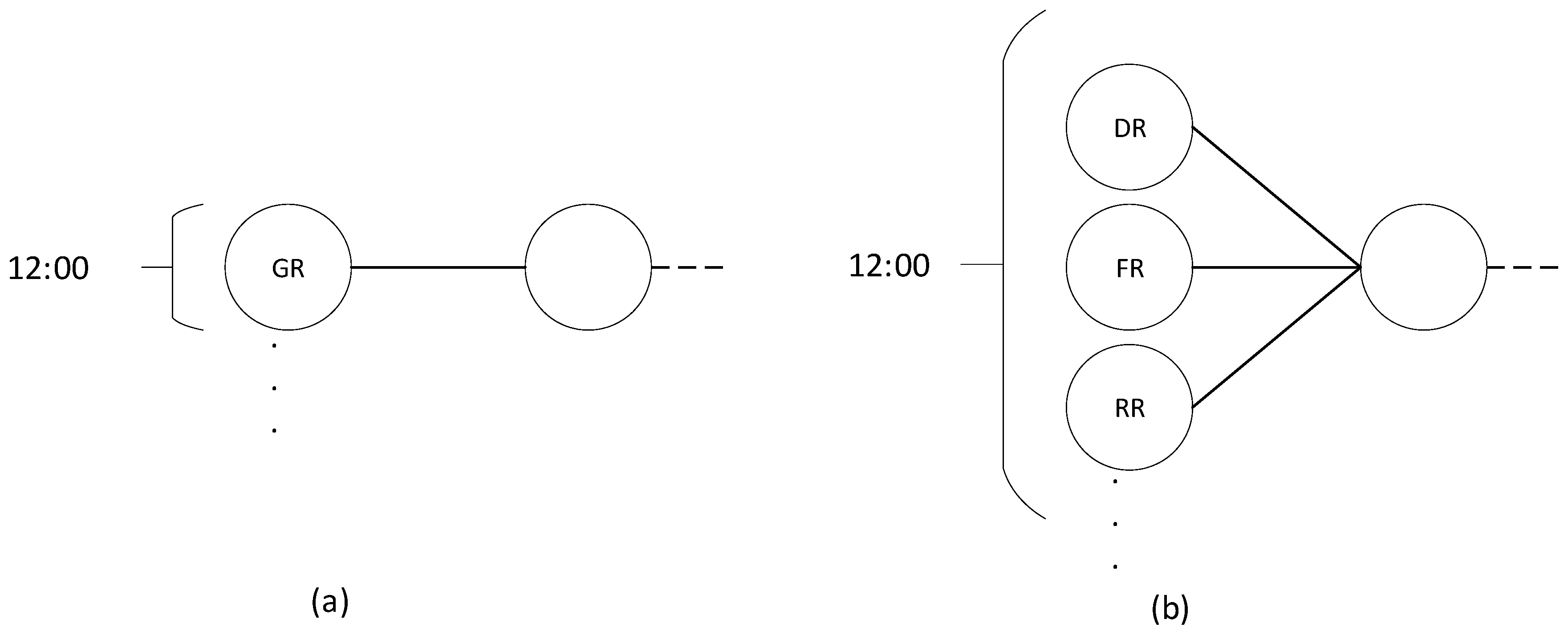
  • Solar forecasting can be done using global energy (GR) as input parameter or it can be separated into its components: directed radiation (DR), diffused radiation (FR), and reflected radiation (RR), as we can see in Figure 3. Depending how this information is provided, the input will have one structure or other.
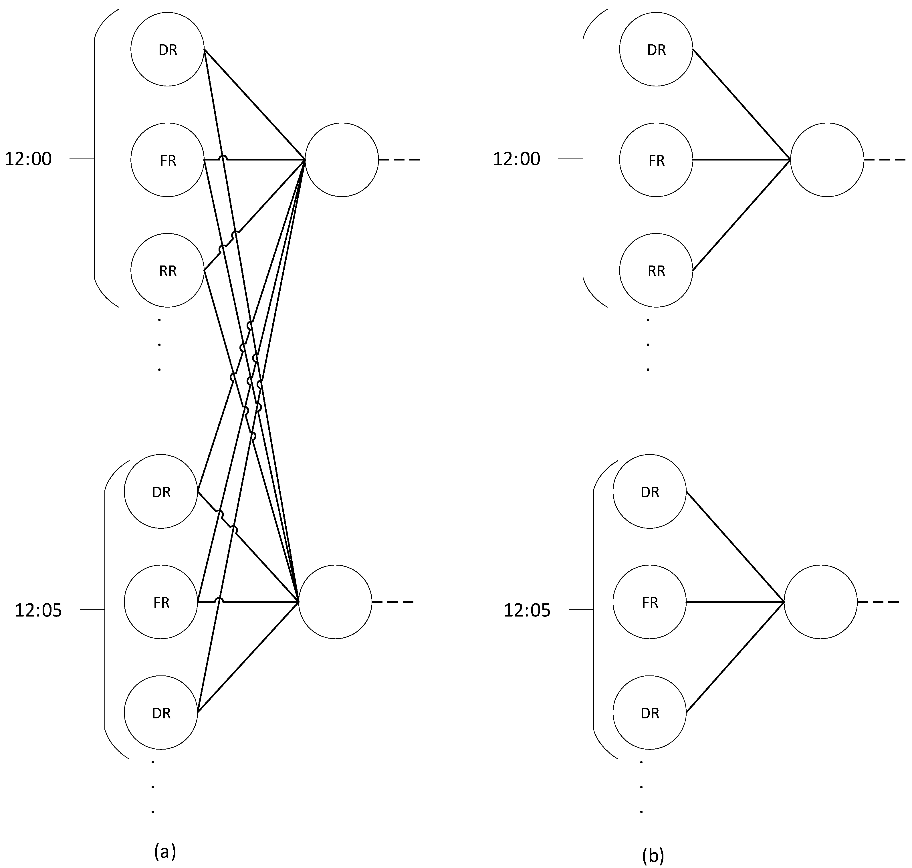
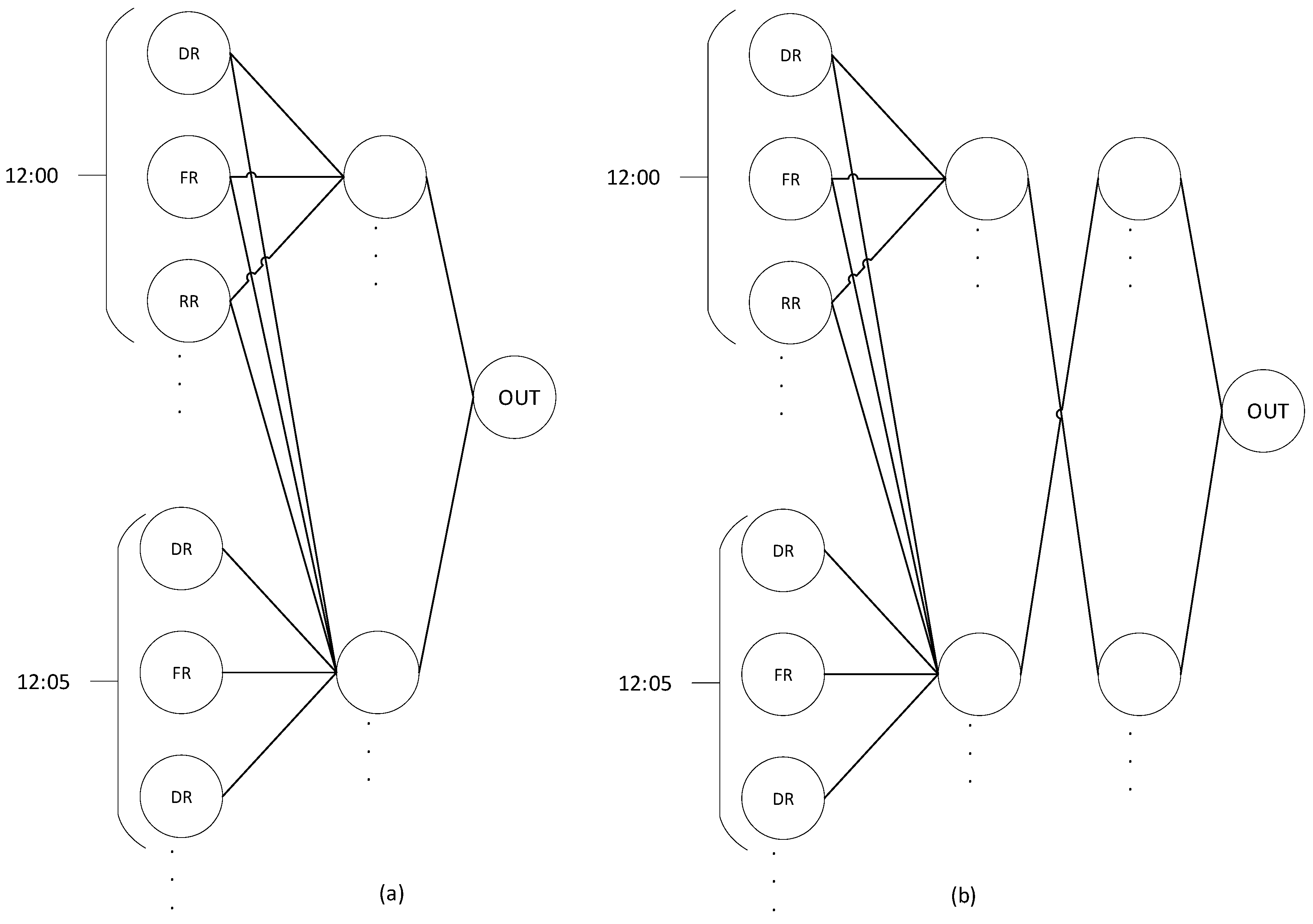
  • Information related about solar parameters provided by the satellites is supplied every 5 min. That information can be connected with a dense layer (where all the information related with solar parameters are interconnected with each other), or we can use a stratified layer to isolate solar radiation data. With this last approach, the solar parameters from one range of time are not interfering in other ranges and it forms an isolated information core (Figure 4).
This approach is used together with broken-down radiation and when an additional layer hidden layer is used (or at least, when is used an additive layer with one neuron). If paired together with global radiation, or if only one hidden layer is used, the stratification does not add predictive capability to the ANN.
  • Number of hidden layers (1 or 2). It has been shown that the number of hidden layers of the ANN can influence the precision of the result, therefore different hypotheses were tested [33]. An additional layer is necessary if broken-down radiation is used, whereas if global radiation is the input element, then only one hidden layer is necessary (Figure 5).
  • Formula for calculating the number of neurons in the hidden layers. It has been shown that the number of neurons in the hidden layers can influence the result, so the number of neurons in the hidden layers was varied, following examples from the literature [34]. The proposed formulas are as follows:
    Hidden = 2 3 ( In + Out )
    Hidden = 3 2 ( In + Out )
    Hidden = 1 2 ( In + Out ) + SQRT ( Training )
    where: In = Number of elements/dimensions in the Input layer, Out = Number of elements/ dimensions on the output layer, Training = Number of samples.
For ANNs with two hidden layers, the number of neurons of this layer was calculated taking in account that the input layer for the formula is the output of the first layer.
In order to summarize, the following table (Table 1) represents different approaches and attributes that each ANN has for every case described above. In order to be able to run each of these ANN, data was adapted attending to the structure of each neural network.
After presenting the different neural network configurations, we provide information about the metrics that were used to evaluate the suitability of the different ANN structures proposed. To know which of the proposed approaches is the most accurate, two statistical parameters that have been used in literature and are well documented in surveys, such as [35] and [36], were used. Additionally, they have been applied in comparative problems of prediction [33], solar power forecasting for smart grid energy management problem [37], and in a system for weather prediction with multiclass support vector machines [38]:
  • MAE (Mean Absolute Error): MAE measures the average magnitude of the errors in a set of predictions, without considering their direction. It is the average over the test sample of the absolute differences between prediction values (A) and real values (B) where all individual differences have equal weight. The mathematical representation is:
    MAE = 1 n = i = 0 n | A i B i |
  • MSE (Mean Squared Error): MSE measures the average magnitude of the squared errors in a set of predictions. As the error is squared, it will be always positive, and the direction of the error is irrelevant. The mathematical representation is:
    MSE = 1 n = i = 0 n ( A i B i ) 2
The experiments were carried out using an Intel Pentium i9-7920X CPU 2.90 GHz, with 64 Gb RAM and 12 cores and 2 NVIDIA GeForce RTX 2080 Ti. Each training run for every approach tested lasted around 8 h.

5. Results, Discussion, and Limitations

In this section, we present a comparison of the results obtained by the different configurations of neural networks that we described, with the statistical parameters cited in Section 4.2. In order to avoid overfitting, we analyze the evolution of the train and test value for every iteration, selecting the optimal number of iterations.
Only the graphic result with the best approach is shown in this section (Figure 6). The rest can be found in the Appendix A.
As can be seen in the result charts, results vary significantly depending on the ANN structure selected. The approach with a dense layer obtains the worst results, as MAE and MSE are greater than 0.04 and 0.2, respectively. This result can be expected since solar radiation may vary significantly depending on the range of time, which denotes that each range of time should be completely isolated from other ranges. In general, all experiments using a stratified layer obtain better results than all the approaches based on dense connection.
Another aspect to take in account is whether radiation should be decomposed. According to the general results obtained, decomposed radiation provides better results than global radiation. The only exception is approach number 8, which has good MSE and MAE values. According to the results, it seems that the ANN can find relationships between the different elements that conform the solar radiation. In this way, the overall performance gets better when broken-down solar data is used. It is noteworthy that all approaches that use decomposed solar radiation use a stratified layer.
Finally, the different formulas used for calculating the number of neurons in hidden layers in every approach only present slight differences in performance. On dense layer connections the results are not conclusive (some of the approaches have slight accuracy improvements, whereas other approaches obtain worse results). However, on stratified layer we always obtain slight improvements.
We must highlight that approach number 13 (stratified layer, two hidden layers, and decomposed radiation) provides the best result of the whole experiment. It obtains significantly lower error values on both metrics (MSE ≈ 0.04 and MAE ≈ 0.16) compared to the initial approaches. Translated into accuracy, this means an average error of ±16% on energy production forecasting, tested over one installation for each country, whose data has not been fed as input to the model (four in total).

5.1. ANN Topologies Results

In this subsection, we present the specific results obtained by all the alternative ANN layouts that we have tested. Furthermore, we also provide a discussion on the performance of each of the models and their particularities. If the different alternatives are not considered relevant, Section 5.2 compares the result of our best performing model with state-of-the-art approaches.
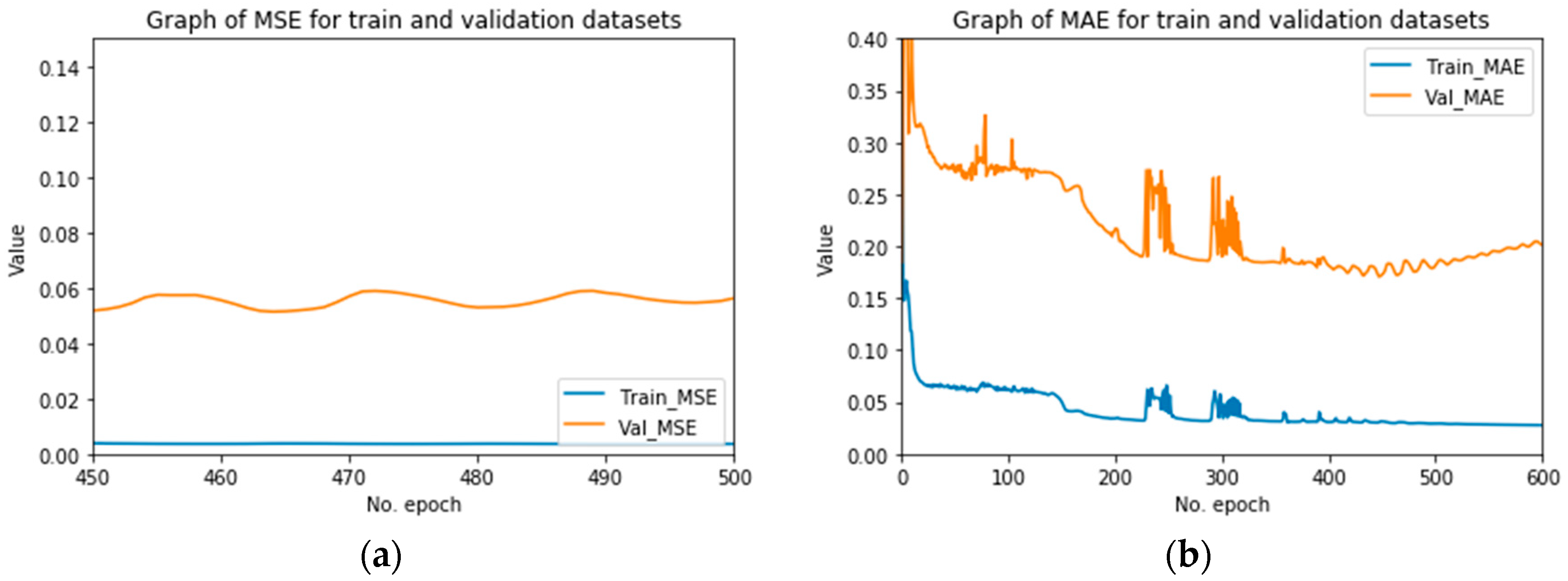
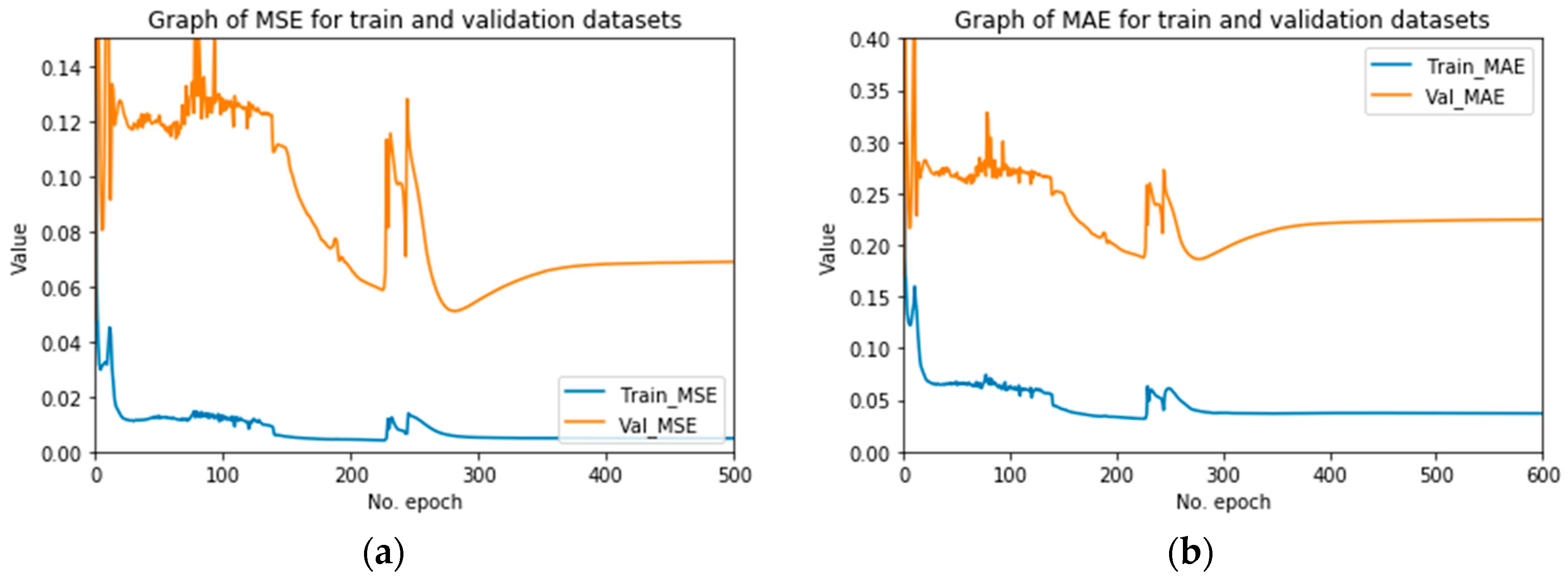
  • In approach 1, we can see oscillations in the training and validation datasets. In addition, it must be pointed that optimal iterations are centered around 500 epochs. From that point on, the validation dataset loses its minimum error value (0.2) and starts to grow.
  • Approach 2 is very similar to the previous one. Global radiation, number of hidden layers, and dense connections are maintained (it changes the formula used for the number of neurons on the hidden layer). As we can see in the figures in the Appendix A, there are greater oscillations in MSE and MAE values than in the previous case, with similar results. As a result, this approach would be worse than previous one.
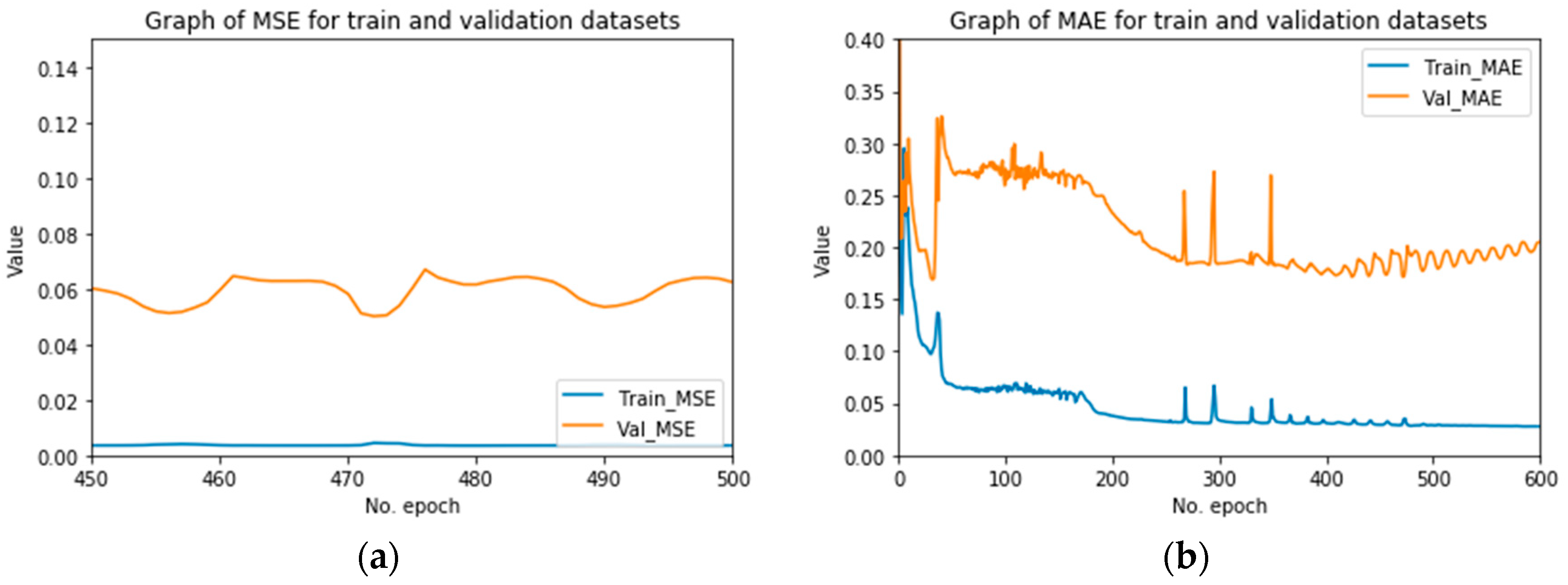
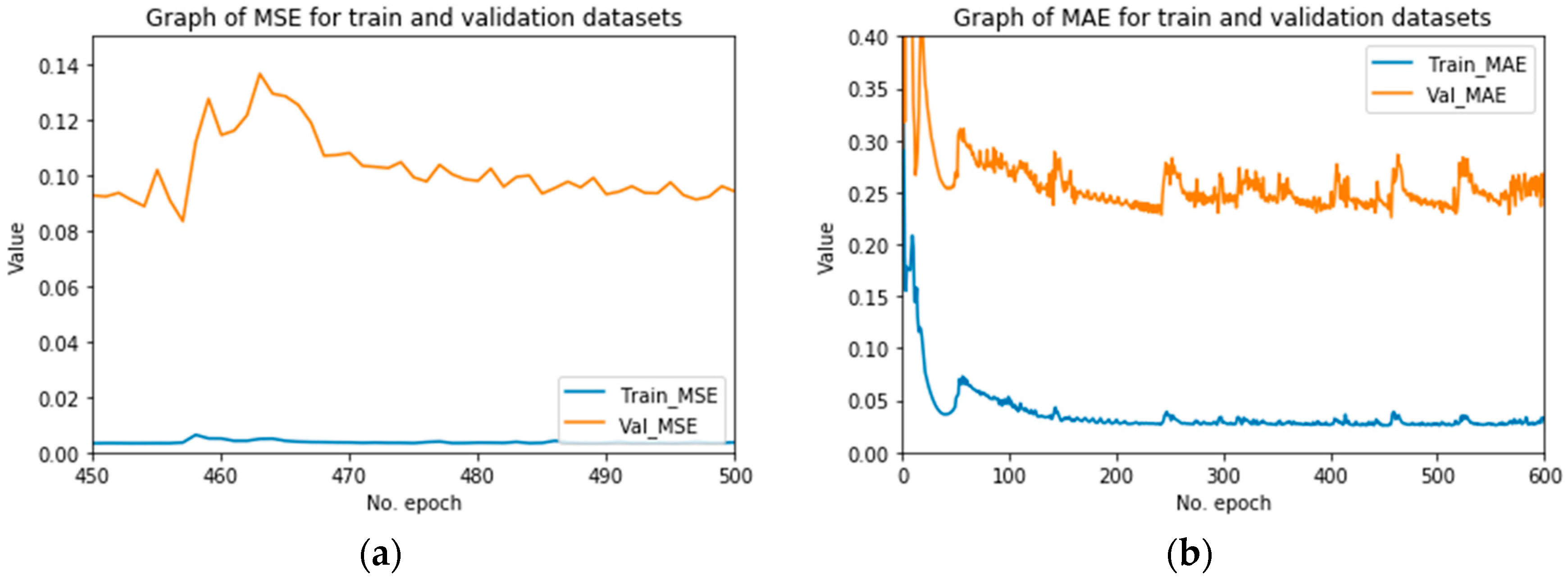
  • In approach 3, we can see oscillations on the initial phases of the training/test phases, until it smooths from epoch 300 onwards. However, the results are not interesting, due to higher values of MSE and MAE (0.067 and 0.024, respectively).
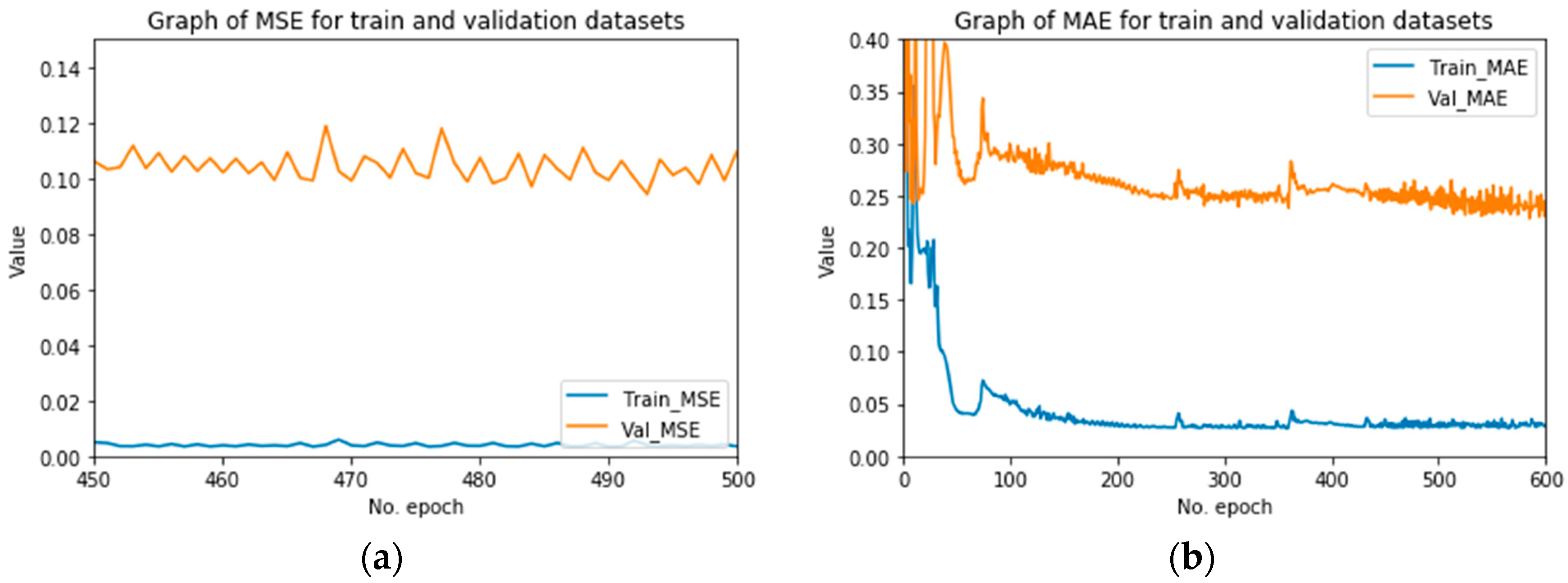
  • Approach 4 is the first pair of graphs with the dense layer connection and decomposed radiation. As it can be easily seen, there are too many oscillations, due to the fully connected approach with the decomposed radiation that conforms a huge multidimensional space of possibilities. Thus, the distribution function can be very difficult to learn properly. In addition, the results are not interesting due to higher values of MSE and MAE (0.10 and 0.27, respectively).
  • Similar to the previous case, there are too many oscillations in approach 5. As a result, we can conclude that the formula used for calculating the number of neurons on hidden layer is less important than other parameters. As in the previous case, error values are relatively higher compared to best performing topologies.
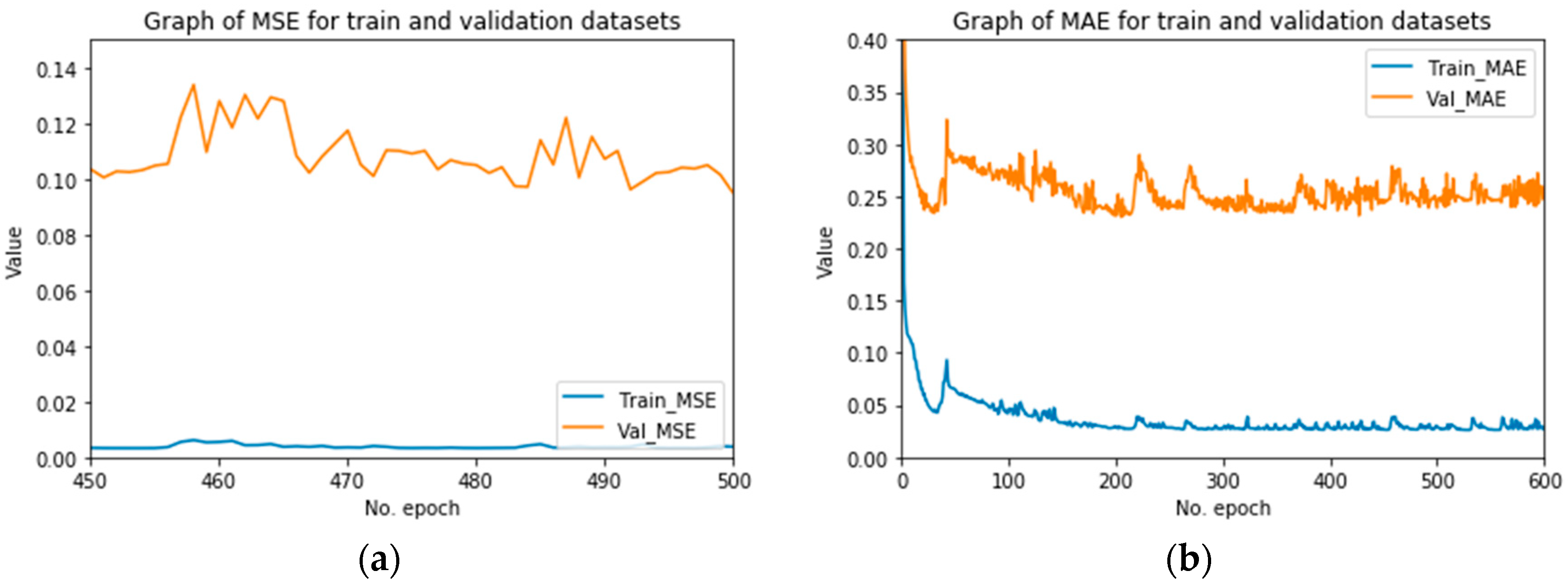
  • The third approach with dense layer and decomposed radiation is reflected in approach 6. It follows the trend of the other two: too many oscillations and elevated values of MSE (0.11) and MAE (0.27) for the validation dataset.
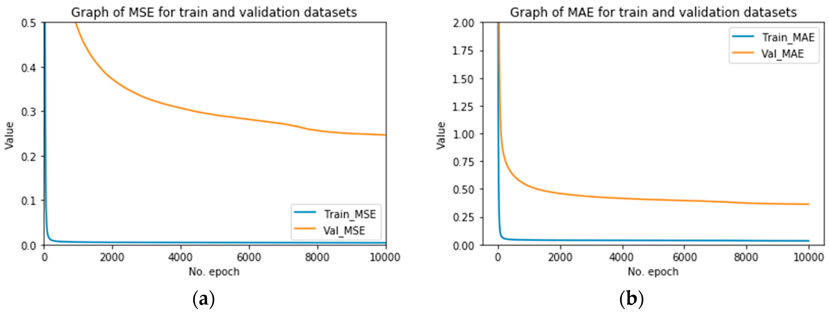
  • Approach 7 is a hybrid of topologies with one hidden layer and topologies with two hidden layers. In this approach, we are using decomposed radiation, but only a simple add layer is used to obtain the distribution function. As it can be observed in the provided figures, the results are the worst across all the topologies, and they must be represented with a different scale.
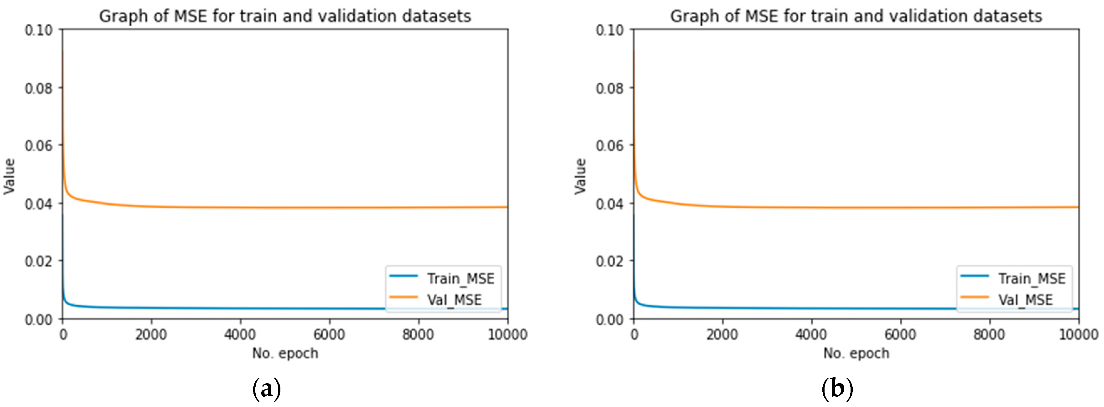
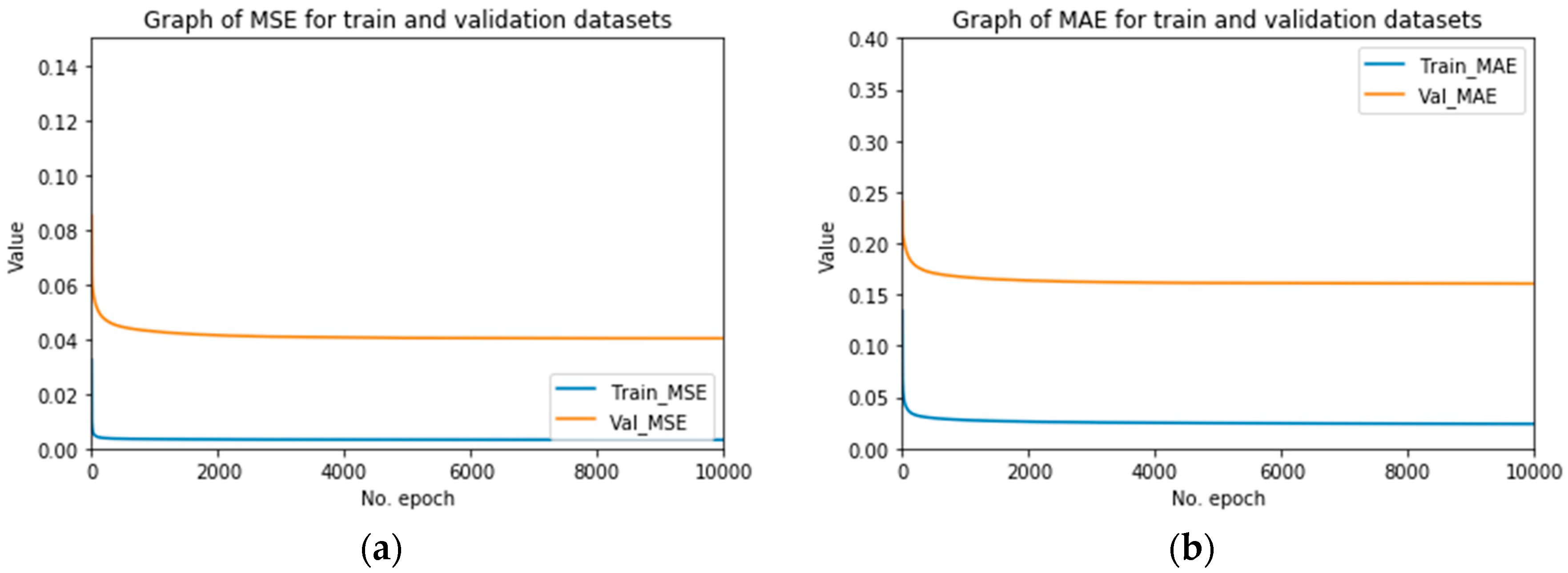
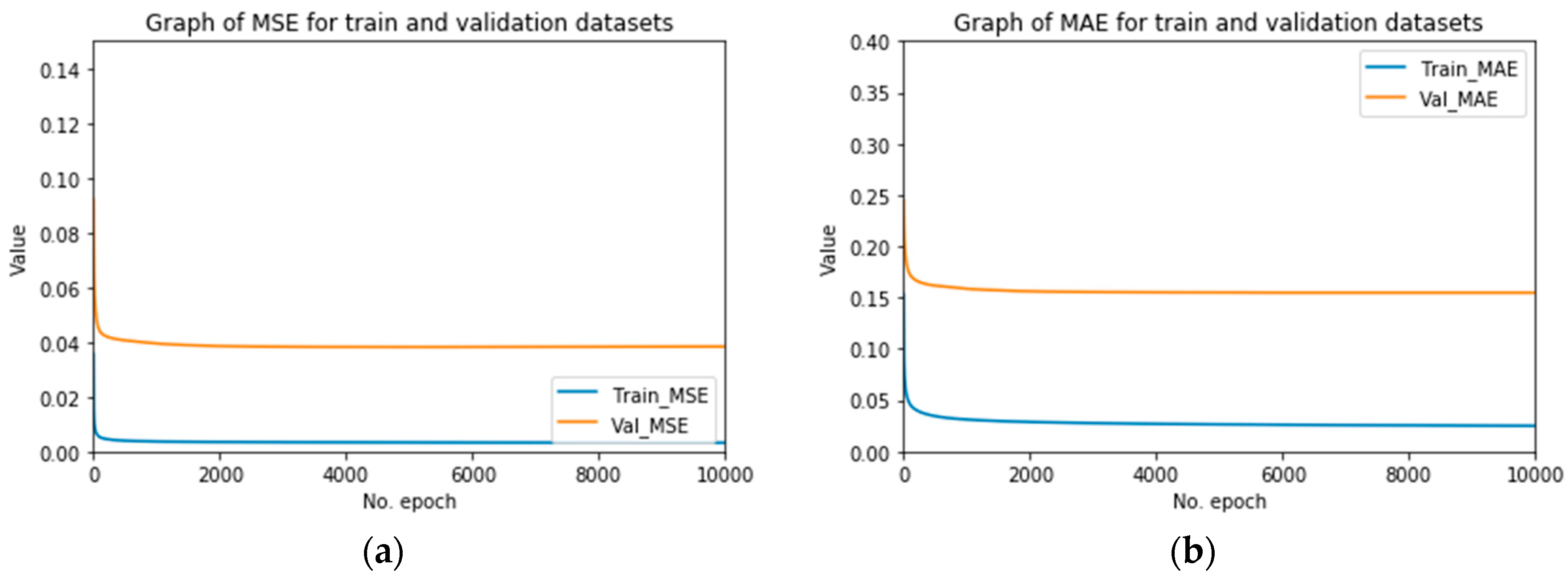
  • In approach 8, we find the first pair of figures with the stratified layer connection and global radiation approach. We can observe in the graphs that the optimal value of test is acquired with a notably higher number of epochs than in previous cases (10,000 vs 500). However, the oscillations have disappeared, and the results are quite more promising, with lower values of MSE and MAE (0.046 and 0.18, respectively).
  • The figures that we can see in approach 9 follow the trends of previous one. With the modification of the number of neurons in the hidden layers, we try to tune the algorithm, in order to provide better results. However, the results are not clearly improved.
  • Same as in the previous approach, with the modification of number of neurons in the hidden layers, we try to tune the algorithm, in order to provide better results. Nevertheless, with the formula used, the results are clearly worse in approach 10 than in the previous approach.
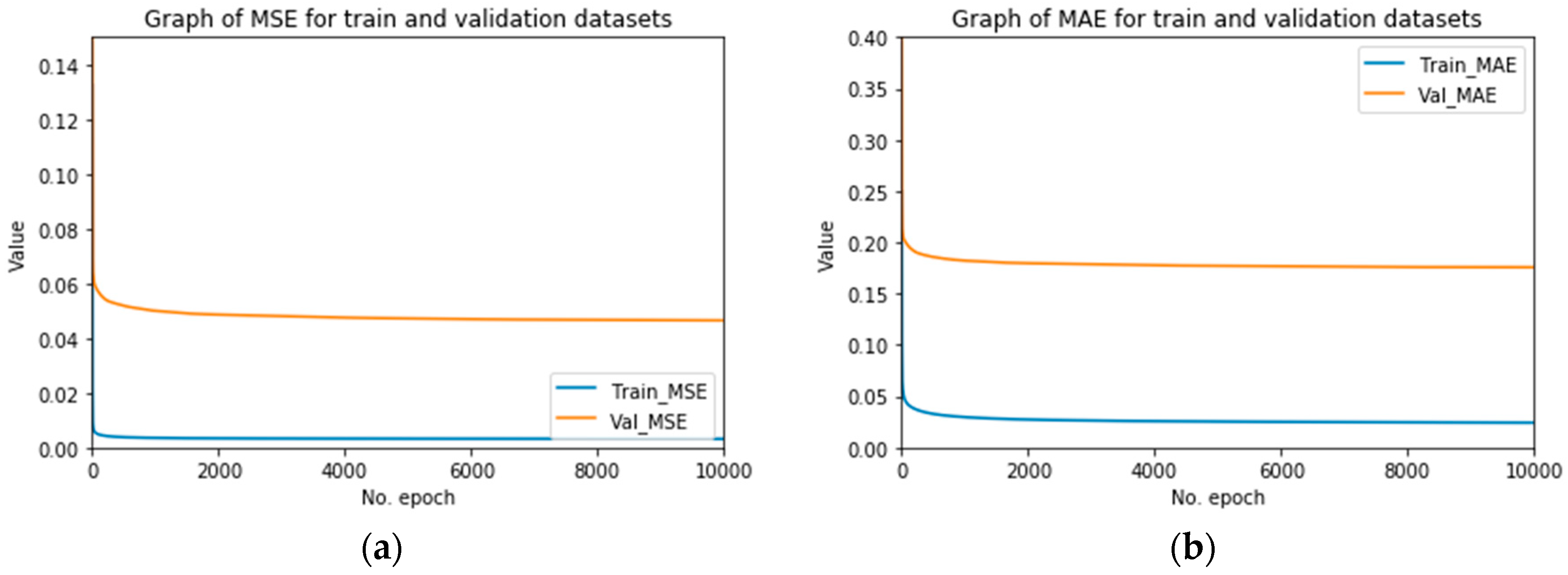
  • To start closing up the analysis of the Appendix A, we present the three approaches based on stratified layer and decomposed radiation, starting with approach 11. As we can see in the graphs, these approaches obtain similar values to the best approach until now (approach 9), with similar values in MSE and MAE (0.04646 and 0.1757, respectively).
  • In approach 12, we are tuning the parameters of number of hidden neurons, looking for slight improvements on MAE and MSE. With the second formula, the results are not clearly improved compared to previous cases.
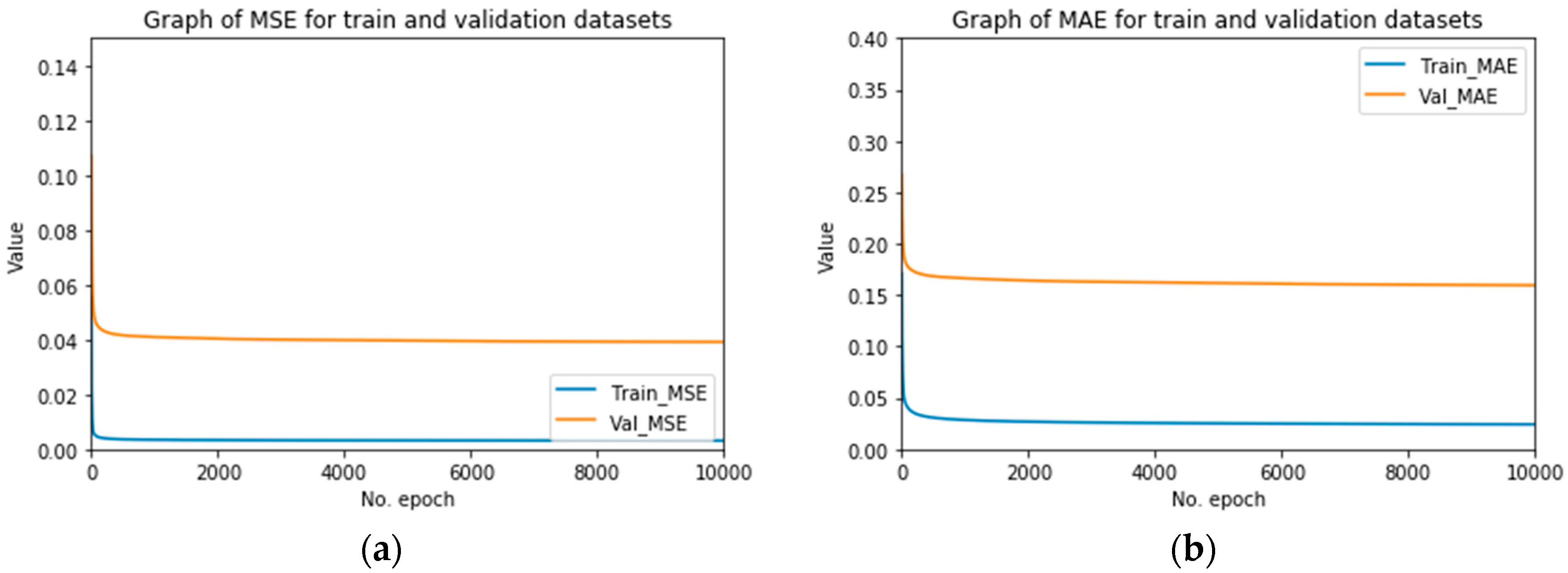
  • Finally, in approach 13, we are tuning the parameter of the number of hidden neurons, looking at slight improvements on MAE and MSE. These results slightly improve the MSE and MAE value obtained in approach 8, obtaining 0.0161 (vs. 0.1757) and 0.04025 (vs. 0.04646), respectively. Thus, these results make this ANN configuration the best one out of the studied topologies.

5.2. Results Compared to the State-Of-The-Art

There are several approaches published in the literature for solar radiation and solar energy prediction. However, the comparability across approaches is limited due to several discrepancies that we must highlight.
First, the interval of predictions is different across approaches. We predict energy up to 5-min intervals, whereas other approaches provide a daily or monthly basis. This is not a limitation in our case, since intervals can be aggregated. However, it is not possible to de-aggregate daily and monthly predictions into smaller intervals.
Second, our approach predicts solar energy (output), whereas many of the other approaches focus on predicting solar radiation (input). There are only few proposals that try to predict solar energy.
Third, our approach is generic, and has been tested with several installations with different characteristics in different locations. Other approaches in the literature focus on a single location, and thus can provide more accurate results at the cost of generalizability.
Taking these aspects into account, we present the comparison of results in Table 2.
As we can see in the table, the best MSE result obtained by approaches in the literature that predict solar energy is within the range from 0.069 to 0.055 [24]. This is slightly less performing than our model, which obtained an MSE of 0.040. In addition, the prediction is daily or monthly, whereas our model is capable of producing 5-min-interval predictions, thus offering higher flexibility.
For those solar energy prediction approaches where MSE is not available and MAE is used instead, we obtained a competitive result. In [25], the authors presented different results for different seasons and ranges of time, ranging from MAE = 12.2% in Spring to MAE = 26.6% from April to September. Compared to these results, our approach obtained an MAE ≈ 0.161 for a whole year of daily predictions. As before, our approach presents higher flexibility, allowing for 5-min-interval predictions or up to daily and monthly basis.
Finally, the proposal in [6] was selected as the main representative of proposals that predict solar radiation instead of solar energy output. This proposal focused on the location of Algeria, and obtained an MSE in the range of 0.157 to 0.0418. Our approach would stay competitive, with an MSE of 0.040 that would be located in the upper (worst) end of the range. However, compared to these results, our approach not only remains more flexible and is more generic (considers multiple locations), but also predicts solar energy output, which has to take into account the characteristics and effect of solar panels and additional weather conditions.
As aforementioned, these results should be taken carefully, since each of the approaches uses their own dataset due to the absence of an existing benchmark. Moreover, most of the approaches make use of private data, which makes it difficult to reuse the same datasets for testing purposes.

5.3. Discussion and Limitations

Although our approach presents several advantages compared to the state of the art, we must still point out some of its own problems and limitations.
First, a critical mass of data is needed in order to achieve a proper training and test of the model for other locations than those that have already been considered in this paper. This can require some training time and resources. In our case the training process took 8 h, without account for the preprocessing of the data and the creation of all the different ANN layouts. Moreover, if a certain feature is not available or a new one was to be added, the retrain process would be mandatory.
The second limitation is the existing threats to the validity of the results. Although we have performed several tests with several countries, the absence of suitable benchmarks makes it difficult to properly compare existing techniques and approaches. Moreover, due to the specification degree required and the quantity of variables involved, such as granularity of the prediction, metrics used, and whether solar radiation or solar energy production is predicted, it is difficult to obtain a quantitative value to discriminate between existing approaches. This also emphasizes the need for the creation of a proper benchmark for future solar models that try to predict solar energy production.

6. Conclusions

Most research so far has focused on predicting solar radiation, rather than focusing on solar energy production forecasting. However, the conversion of solar radiation into solar energy power is far from trivial. Solar energy is influenced by factors such as temperature, wind, or the solar panels used, adding an extra layer of complexity over solar radiation. As a result, users do not have a clear idea how much solar energy output can be expected, and how much they should invest in an installation according to their location and the characteristics of the solar panels to be bought.
In this paper we have presented a model that provides a solution for users and authorities interested in sustainable energy power forecasting based on solar power. Our approach presents an ANN structure that has been tested with different topologies and provides solar energy forecasting with data that has been obtained from Open Data sources. Compared to existing approaches, it presents the following advantages:
  • It is trained with Open Data. Consequently, everyone with proper technical knowledge can access the data sources and get the data for building their own ANN model.
  • It is focused on solar power forecasting, rather than solar radiation prediction. As a result of that, we can answer high-level questions (focused on return on investment (ROI) of the installation), thanks to the abstraction layer that has been included between solar radiation and its conversion to solar power.
  • It provides solid accuracy results. The presented method provides competitive results on MAE and MSE metrics compared to other approaches that we have found in the literature.
In this way, our approach can be applied widely as long as there is Open Data published for the location, simply re-training or tuning the presented model. Moreover, our model can be modified to predict solar energy production on specific hour fragments, since its resolution is much higher than existing models.
In addition, another advantage of the presented model is the speed to generate new forecasts. Due to the fact that the ANN is already trained, the computation of a new prediction can be done in just a few seconds if all the data required is provided.
Furthermore, with the proliferation of IoT in solar power installations, data generated will increase considerably in the next years. As a result, our algorithm will become more accurate and precise.
Besides that, it must be pointed out that with a few modifications on the ANN proposed, the model can be tuned to predict energy solar production in specific hour fragments.
This proposal allows users to predict, given an installation and the solar energy received over a period of time, the energy generation of the installation for those specific ranges of time under normal conditions, accessing the corresponding data in the cited references.
Finally, while we have tested our approach with a variety of solar installations, the system can be specialized to focus on specific installation types, thus likely increasing its accuracy. For instance, a user could focus on installations with specific sizes or specific types of solar panel. Nevertheless, this still requires providing all the necessary information to train the ANN, which may or may not be available for that specific installation.
Nevertheless, there is still much work to be done in the area. For instance, a large, curated dataset would lead to increased accuracy in the predictions as well as foster investment in the area. Moreover, while we have focused on solar energy, the approach could be extended to other sustainable energies, such as wind-based energy production.
To this aim, our future work is focused on fostering sustainable energy self-supplying, by using open data provided by different administrations to analyze the self-sufficiency capabilities of a village or town. This way, we can provide information in advance about when and how much non-renewable energy will be needed to cover the gap until all energy demand can be covered.

Author Contributions

Conceptualization, J.M.B., A.R., A.M. and J.C.T.; Data curation, A.R.; Formal analysis, J.M.B. and A.R.; Methodology, J.M.B., A.R., A.M. and J.C.T.; Project administration, A.M.; Resources, J.C.T.; Software, J.M.B., A.R., A.M. and J.C.T.; Validation, J.M.B. and A.R.; Writing—original draft, J.M.B. and A.R.; Writing—review & editing, A.M. and J.C.T. All authors have read and agreed to the published version of the manuscript.

Funding

This paper has been co-funded by the ECLIPSE-UA (RTI2018-094283-B-C32) project from the Spanish Ministry of Science, Innovation, and Universities; both Jose M. Barrera (I-PI 98/18) and Alejandro Reina (I-PI 13/20) hold an Industrial PhD Grants co-funded by the University of Alicante and the Lucentia Lab Spin-off Company.

Acknowledgments

We would like to thank the Lucentia Lab Spin-off Company for providing us with all the support, algorithms, and the data necessary for the application of our proposal.

Conflicts of Interest

The authors declare no conflict of interest.

Appendix A

This section presents the results for all the approaches.
Figure A1. Approach 1: Dense layer. Formula (1). Hidden layers = 1. Global radiation. (a) MSE. (b) MAE.
Sustainability 12 06915 g0a1
Figure A2. Approach 2: Dense layer. Formula (2). Hidden layers = 1. Global radiation. (a) MSE. (b) MAE.
Sustainability 12 06915 g0a2
Figure A3. Approach 3: Dense layer. Formula (3). Hidden layers = 1. Global radiation. (a) MSE. (b) MAE.
Sustainability 12 06915 g0a3
Figure A4. Approach 4: Dense layer. Formula (1). Hidden layers = 1. Decomposed radiation. (a) MSE. (b) MAE.
Sustainability 12 06915 g0a4
Figure A5. Approach 5: Dense layer. Formula (2). Hidden layers = 1. Decomposed radiation. (a) MSE. (b) MAE.
Sustainability 12 06915 g0a5
Figure A6. Approach 6: Dense layer. Formula (3). Hidden layers = 1. Decomposed radiation. (a) MSE. (b) MAE.
Sustainability 12 06915 g0a6
Figure A7. Approach 7: Stratified layer. Add layer Hidden layers = 1. Decomposed radiation. (a) MSE. (b) MAE.
Sustainability 12 06915 g0a7
Figure A8. Approach 8: Stratified layer. Formula (1). Hidden layers = 2. Global radiation. (a) MSE. (b) MAE.
Sustainability 12 06915 g0a8
Figure A9. Approach 9: Stratified layer. Formula (2). Hidden layers = 2. Global radiation. (a) MSE. (b) MAE.
Sustainability 12 06915 g0a9
Figure A10. Approach 10: Stratified layer. Formula (3) Hidden layers = 2. Global radiation. (a) MSE. (b) MAE.
Sustainability 12 06915 g0a10
Figure A11. Approach 11: Stratified layer. Formula (1) Hidden layers = 2. Decomposed radiation. (a) MSE. (b) MAE.
Sustainability 12 06915 g0a11
Figure A12. Approach 12: Stratified layer. Formula (2) Hidden layers = 2. Decomposed radiation. (a) MSE. (b) MAE.
Sustainability 12 06915 g0a12
Figure A13. Approach 13: Stratified layer. Formula (3) Hidden layers = 2. Decomposed radiation. (a) MSE. (b) MAE.
Sustainability 12 06915 g0a13

References

  1. Shafeek, H. Maintenance Practices in Cement Industry. Asian Trans. Eng. 2012, 1, 10–20. [Google Scholar]
  2. Kiesecker, J.; Baruch-Mordo, S.; Heiner, M.; Negandhi, D.; Oakleaf, J.R.; Kennedy, C.M.; Chauhan, P. Renewable Energy and Land Use in India: A Vision to Facilitate Sustainable Development. Sustainability 2019, 12, 281. [Google Scholar] [CrossRef] [Green Version]
  3. King, P.; Sansom, C.; Comley, P. Photogrammetry for Concentrating Solar Collector Form Measurement, Validated Using a Coordinate Measuring Machine. Sustainability 2019, 12, 196. [Google Scholar] [CrossRef] [Green Version]
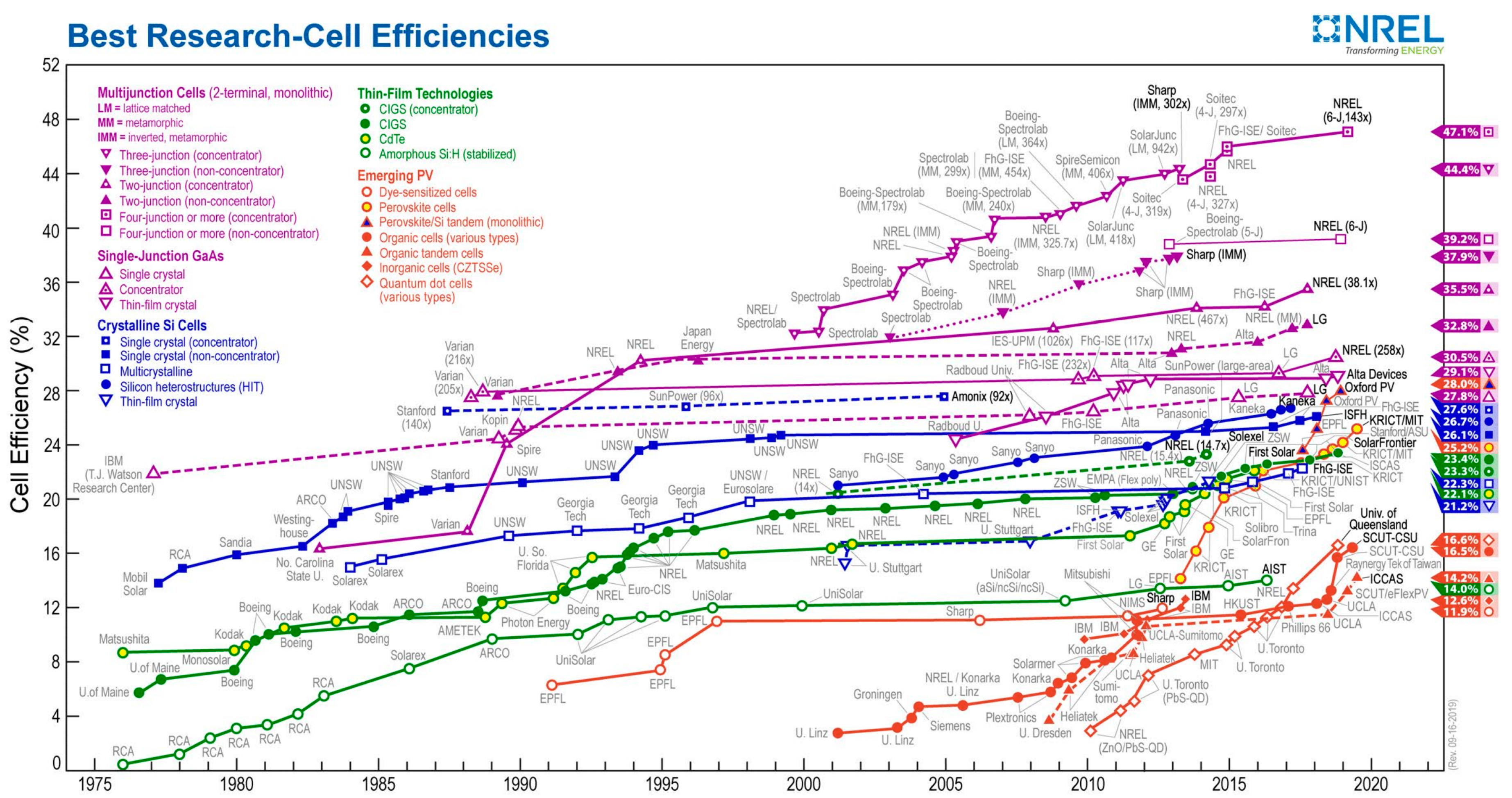
  4. National Renewable Energy Laboratory. Best Research-Cell Efficiency Chart: Photovoltaic Research. Available online: https://www.nrel.gov/pv/cell-efficiency.html (accessed on 21 February 2020).
  5. Noticias CIEMAT: El CIEMAT Presenta en Alpedrete el Mapa Solar del Municipio. Available online: http://www.ciemat.es/cargarAplicacionNoticias.do;jsessionid=E2015D198EA7C11FCD180ACB22A03F3C?idArea=-1&identificador=1500 (accessed on 24 August 2020).
  6. Nia, M.; Chegaar, M.; Benatallah, M.F.; Aillerie, M. Contribution to the quantification of solar radiation in Algeria. Energy Procedia 2013, 36, 730–737. [Google Scholar] [CrossRef]
  7. Gautier, C.; Diak, G.; Massé, S. A Simple Physical Model to Estimate Incident Solar Radiation at the Surface from GOES Satellite Data. J. Appl. Meteorol. 1980, 19, 1005–1012. [Google Scholar] [CrossRef] [Green Version]
  8. Chineke, T.C. Equations for estimating global solar radiation in data sparse regions. Renew. Energy 2008, 33, 827–831. [Google Scholar] [CrossRef]
  9. Khatib, T.; Mohamed, A.; Mahmoud, M.M.; Sopian, K. Modeling of Daily Solar Energy on a Horizontal Surface for Five Main Sites in Malaysia. Int. J. Green Energy 2011, 8, 795–819. [Google Scholar] [CrossRef]
  10. Li, H.; Ma, W.; Wang, X.; Lian, Y. Estimating monthly average daily diffuse solar radiation with multiple predictors: A case study. Renew. Energy 2011, 36, 1944–1948. [Google Scholar] [CrossRef]
  11. Şen, Z. Simple nonlinear solar irradiation estimation model. Renew. Energy 2007, 32, 342–350. [Google Scholar] [CrossRef]
  12. Akinoǧlu, B.; Ecevit, A. Construction of a quadratic model using modified Ångstrom coefficients to estimate global solar radiation. Sol. Energy 1990, 45, 85–92. [Google Scholar] [CrossRef]
  13. Şen, Z. Angström equation parameter estimation by unrestricted method. Sol. Energy 2001, 71, 95–107. [Google Scholar] [CrossRef]
  14. Rizwan, M.; Jamil, M.; Kirmani, S.; Kothari, D. Fuzzy logic based modeling and estimation of global solar energy using meteorological parameters. Energy 2014, 70, 685–691. [Google Scholar] [CrossRef]
  15. Chugh, A.; Chaudhary, P.; Rizwan, M. Fuzzy logic approach for short term solar energy forecasting. In Proceedings of the 12th IEEE International Conference Electronics, Energy, Environment, Communication, Computer, Control: (E3-C3) INDICON, Piscataway, NJ, USA, 17–20 December 2015. [Google Scholar]
  16. Monís, J.I.; López-Luque, R.; Reca, J.; Martínez, J. Multistage Bounded Evolutionary Algorithm to Optimize the Design of Sustainable Photovoltaic (PV) Pumping Irrigation Systems with Storage. Sustainability 2020, 12, 1026. [Google Scholar] [CrossRef] [Green Version]
  17. Che, S.; Boyer, M.; Meng, J.; Tarjan, D.; Sheaffer, J.W.; Skadron, K. A performance study of general-purpose applications on graphics processors using CUDA. J. Parallel Distrib. Comput. 2008, 68, 1370–1380. [Google Scholar] [CrossRef]
  18. Jin, L.; Kuang, X.; Huang, H.; Qin, Z.; Wang, Y. Study on the Overfitting of the Artificial Neural Network Forecasting Model. J. Meteorol. Res. 2005, 19, 216–225. [Google Scholar]
  19. Karatepe, E.; Boztepe, M.; Colak, M. Neural network based solar cell model. Energy Convers. Manag. 2006, 47, 1159–1178. [Google Scholar] [CrossRef]
  20. Fadare, D. Modelling of solar energy potential in Nigeria using an artificial neural network model. Appl. Energy 2009, 86, 1410–1422. [Google Scholar] [CrossRef]
  21. Mellit, A.; Benghanem, M.; Bendekhis, M. Artificial neural network model for prediction solar radiation data: Application for sizing stand-alone photovoltaic power system. In Proceedings of the 2005 IEEE Power Engineering Society General Meeting, San Francisco, CA, USA, 12–16 June 2005; Volume 1, pp. 40–44. [Google Scholar]
  22. Amrouche, B.; Le Pivert, X. Artificial neural network based daily local forecasting for global solar radiation. Appl. Energy 2014, 130, 333–341. [Google Scholar] [CrossRef]
  23. Quiles, E.; Roldán-Blay, C.; Escrivá-Escrivá, G.; Porta, C.R. Accurate Sizing of Residential Stand-Alone Photovoltaic Systems Considering System Reliability. Sustainability 2020, 12, 1274. [Google Scholar] [CrossRef] [Green Version]
  24. Abuella, M.; Chowdhury, B. Solar power forecasting using artificial neural networks. In Proceedings of the 2015 North American Power Symposium, Charlotte, NC, USA, 4–6 October 2015. [Google Scholar]
  25. Cococcioni, M.; D’Andrea, E.; Lazzerini, B. 24-h-ahead forecasting of energy production in solar PV systems. In Proceedings of the 11th International Conference on Intelligent Systems Design and Applications, Cordoba, Spain, 22–24 November 2011; pp. 1276–1281. [Google Scholar]
  26. Gala, Y.; Fernández, A.; Dorronsoro, J.; García, M.; Rodríguez, C. Machine Learning Prediction of Global Photovoltaic Energy in Spain. Renew. Energy Power Qual. J. 2014, 605–610. [Google Scholar] [CrossRef]
  27. Ibrahim, S.; Daut, I.; Irwan, Y.; Irwanto, M.; Gomesh, N.; Farhana, Z. Linear Regression Model in Estimating Solar Radiation in Perlis. Energy Procedia 2012, 18, 1402–1412. [Google Scholar] [CrossRef] [Green Version]
  28. Dupré, O.; Vaillon, R.; Green, M.A. Thermal Behavior of Photovoltaic Devices; Springer Science and Business Media: Berlin/Heidelberg, Germany, 2017. [Google Scholar]
  29. Jacques, S.; Caldeira, A.; Ren, Z.; Schellmanns, A.; Batut, N. Impact of the cell temperature on the energy efficiency of a single glass PV module: Thermal modeling in steady-state and validation by experimental data. Renew. Energy Power Qual. J. 2013, 1, 291–294. [Google Scholar] [CrossRef]
  30. Uhlir, P.F.; Schröder, P. Open Data for Global Science. Data Sci. J. 2007, 6, OD36–OD53. [Google Scholar] [CrossRef] [Green Version]
  31. PVOutput. Available online: https://pvoutput.org/ (accessed on 10 March 2020).
  32. EU Science Hub. Photovoltaic Geographical Information System (PVGIS). Available online: https://ec.europa.eu/jrc/en/pvgis (accessed on 24 August 2020).
  33. Behera, M.K.; Nayak, N. A comparative study on short-term PV power forecasting using decomposition based optimized extreme learning machine algorithm. Eng. Sci. Technol. Int. J. 2020, 23, 156–167. [Google Scholar] [CrossRef]
  34. Shaft, I.; Ahmad, J.; Shah, S.I.; Kashif, F.M. Impact of varying neurons and hidden layers in neural network architecture for a time frequency application. In Proceedings of the 10th IEEE International Multitopic Conference (INMIC), Islamabad, Pakistan, 23–24 December 2006; pp. 188–193. [Google Scholar]
  35. Hyndman, R.J.; Koehler, A.B. Another look at measures of forecast accuracy. Int. J. Forecast. 2006, 22, 679–688. [Google Scholar] [CrossRef] [Green Version]
  36. Kim, S.; Kim, H. A new metric of absolute percentage error for intermittent demand forecasts. Int. J. Forecast. 2016, 32, 669–679. [Google Scholar] [CrossRef]
  37. Wan, C.; Zhao, J.; Song, Y.; Xu, Z.; Lin, J.; Hu, Z. Photovoltaic and solar power forecasting for smart grid energy management. CSEE J. Power Energy Syst. 2015, 1, 38–46. [Google Scholar] [CrossRef]
  38. Zhang, W.; Zhang, H.; Liu, J.; Li, K.; Yang, D.; Tian, H. Weather prediction with multiclass support vector machines in the fault detection of photovoltaic system. IEEE/CAA J. Autom. Sin. 2017, 4, 520–525. [Google Scholar] [CrossRef]
Figure 1. Range of photovoltaic conversion efficiencies of solar panels, from 1976 until present [4].
Sustainability 12 06915 g001
Figure 2. Solar radiation in Earth’s atmosphere [27].
Sustainability 12 06915 g002
Figure 3. Global vs Decomposed radiation structure. (a) Global radiation (b) Decomposed radiation.
Sustainability 12 06915 g003
Figure 4. Dense vs Stratified layer structure. (a) Dense layer (b) Stratified layer.
Sustainability 12 06915 g004
Figure 5. Comparison of layers structure. (a) One hidden layer (b) Two hidden layer.
Sustainability 12 06915 g005
Figure 6. Stratified layer. Formula (3) Hidden layers = 2. Decomposed radiation. (a) Mean Squared Error (MSE). (b) Mean Absolute Error (MAE).
Sustainability 12 06915 g006
Table 1. Summary table with all approaches and their structure.
ApproachDescription
1Dense layer. Formula (1). Hidden layers = 1. Global radiation
2Dense layer. Formula (2). Hidden layers = 1. Global radiation
3Dense layer. Formula (3). Hidden layers = 1. Global radiation
4Dense layer. Formula (1). Hidden layers = 1. Decomposed radiation
5Dense layer. Formula (2). Hidden layers = 1. Decomposed radiation
6Dense layer. Formula (3). Hidden layers = 1. Decomposed radiation
7Stratified layer. Add layer Hidden layers = 1. Decomposed radiation
8Stratified layer. Formula (1) Hidden layers = 2. Global radiation
9Stratified layer. Formula (2) Hidden layers = 2. Global radiation
10Stratified layer. Formula (3) Hidden layers = 2. Global radiation
11Stratified layer. Formula (1) Hidden layers = 2. Decomposed radiation
12Stratified layer. Formula (2) Hidden layers = 2. Decomposed radiation
13Stratified layer. Formula (3) Hidden layers = 2. Decomposed radiation
Table 2. Summary table with results of our approach and other in literature.
ApproachMSEType of PredictionPrediction GranularityMAE
Solar power forecasting using artificial neural networks [24]0.069–0.055EnergyDaily, Monthly-
24-h-ahead forecasting of energy production in solar PV systems [25]-EnergyDailySpring:0.122
Summer:0.211
April–Sept:0.266
Contribution of quantification of solar radiation in Algeria [6]0.0157–0.0418RadiationMonthly-
Solar energy prediction model based on artificial neural networks and open data0.040Energy5 Min,
Daily,
Monthly
0.161

