Concept Design and Performance Evaluation of a Fossil-Free Operated Cargo Ship with Unlimited Range

Abstract

To meet the IMO goals of emissions reduction in shipping, drastic actions must be taken. Wind-assisted propulsion and renewable energy sources are today discussed frequently as realistic alternatives for future ship propulsion and energy production. This study presents a new and innovative concept of a fossil-free operated cargo ship aiming to achieve an unlimited range. The purpose of the study is to present the feasibility but also the limitations of a ship propelled and operated purely on renewable energy harnessed at sea, independent from shore-based energy sources. Aside from Flettner rotors for propulsion, the ship concept incorporates photovoltaic generators, wind turbines, and a dual-mode propeller to produce energy for the auxiliary systems and for the Flettner rotors, as well as batteries to balance the energy production and consumption. The dual-mode propeller can be used for energy generation and propulsion, thus levelling out any speed drops or peaks and thereby ensuring more reliable operation. The whole system is modelled numerically, and full ship voyages are simulated using the ship performance model ShipCLEAN. Results show feasible achieved speeds on a route with realistic weather conditions. However, negative energy balances limit the pure renewable sailing conditions. Further logistic and technical challenges are discussed.

1. Introduction

Global trade is one of the pillars of the modern world, where shipping stands for about 90% of the total cargo volume [1]. Today, ships are mainly powered by fossil fuels, and the combustion is responsible for the emission of pollutant gases such as NOx and SOx and about 3% of the total CO2 emissions. Additionally, it is predicted that emissions will increase between 150–250% until 2050 [2]. Climate change is the main effect caused by emissions and has already become a critical situation for society. In the last decades, renewable energies have been reintroduced in the shipping industry. These energy sources have been incorporated mainly as a complementary technology, hybridizing traditional fossil fuel-powered systems, see e.g., [3,4,5,6,7,8,9,10,11,12], but some projects substitute fossil fuels completely [13].

Some studies have investigated the viability of using the wind to propel ships: [3,4] studied wing sails propulsion, [5] evaluated the application of Flettner rotors, and in [6,7] the benefits of using kites for propulsion were evaluated. In all these studies, the primary conclusion was that fuel consumption can be reduced by 20% to more than 30% for normal sailing conditions in merchant shipping. With the wind as an energy source, [8,9] considered wind turbines to generate electric power. This technology reaches fuel savings of more than 35%, contributing to a relevant reduction of emissions. The study presented in [10] considered a set of solar panels and a battery system as a hybrid electric generator. It is highlighted that the time zone and the local time are the parameters that mainly influence the energy production. In [11,12], the impact of installing a hydro turbine under the ship hull was investigated, showing energy savings of more than 3%. Finally, [13] studied the journey of a fossil-free ship with sails and wave-foils as the main power systems. It was concluded that the achievable speed for a route from Funchal to Punta Delgada was about 5–6 knots with a standard deviation of 4 knots.

The solutions and innovations presented in these studies show a positive impact of alternative propulsion and renewable energies regarding the reduction of emissions and fuel cost. However, to keep today’s shipping schedules, more energy is often required than could be produced by renewable sources. This aspect has not been considered sufficiently in most recent research studies. Thus, the objective of this study is to define the benefits and limitations of a ship purely powered with renewable energy systems by developing a reference concept vessel without fossil fuel technologies and simulate its performance for different routes and weather conditions.

In Section 2, the method used in the study is presented together with the case study vessel. The section explains the modelling of renewable energy systems and its integration with the ship performance prediction model ShipCLEAN to simulate journeys for different routes and weather conditions. In the concept ship design process, ship dimensions and renewable energy system characteristics are defined. Section 3 presents the results of different simulation cases to analyze how weather conditions and restrictions on ship speed influence voyage time and energy consumption. The conclusions of the study are presented in Section 4. The project focuses on the study of the technical and practical feasibility of the installed technology; the economic viability of the project has not been evaluated in the present work.

2. Concept Vessel and Methodology

In this section, a numerical model to calculate the ship speed, energy consumption, and energy production from an established set of renewable systems in a defined meteorological condition is presented. The model was used to evaluate the performance of a ship in variable weather conditions along a route.

The study in [14] demonstrated the potential of the renewable systems used in the present work. Some assumptions have been made regarding the purpose and characteristics of the concept ship during the selection of renewable technologies.

• Low-speed ship: It was assumed that the renewable power possible to obtain from systems installed in a ship is reduced compared to the energetical density of a fossil fuel. This assumption was made when deciding the velocity considered as acceptable on the fossil-free operated ship concept. From a previous study on pure renewable-powered ships ([13]), the speed considered as acceptable is between 5 and 6 knots average speed.
• High blockage hull: The low ship speed considered limits the ship cargo purpose to those ship types carrying cargo with low volume freight price. A high blockage ship hull was assumed for the present study. A high blockage ship is referred to as a tanker ship or bulk carrier, which has speeds that stay in the range between 13 and 18 knots. It was assumed that corresponding speed reduction from a fossil-based to a fossil-free operated ship can be accepted by the market.
• Open deck space: As most of the current existing renewable technologies are installed in the weather deck area, the concept of ship design cannot require the open deck for cargo handling labors. Therefore, the ship type is limited to tanker ships, where cargo can be handled with pipes, or bulk carriers, in which cargo can be handled with side openings.
• Autonomous systems: The systems onboard must be designed to have the minimum impact on the crew operation working autonomously or with minimum interaction.

Additionally, the current study aims to demonstrate the applicability of the ship performance model ShipCLEAN [15] to define and simulate the propulsion system of the fossil-free concept ship with wind technologies as the main propulsor. From the ship dimensions, the wind propulsion system characteristics and weather conditions, ShipCLEAN evaluated the equilibrium of forces and moments in 4 degrees of freedom (surge, sway, yaw, and heel) and predicted the obtained ship speed and energy demand for the rotors for pure sailing (see Section 2.1). 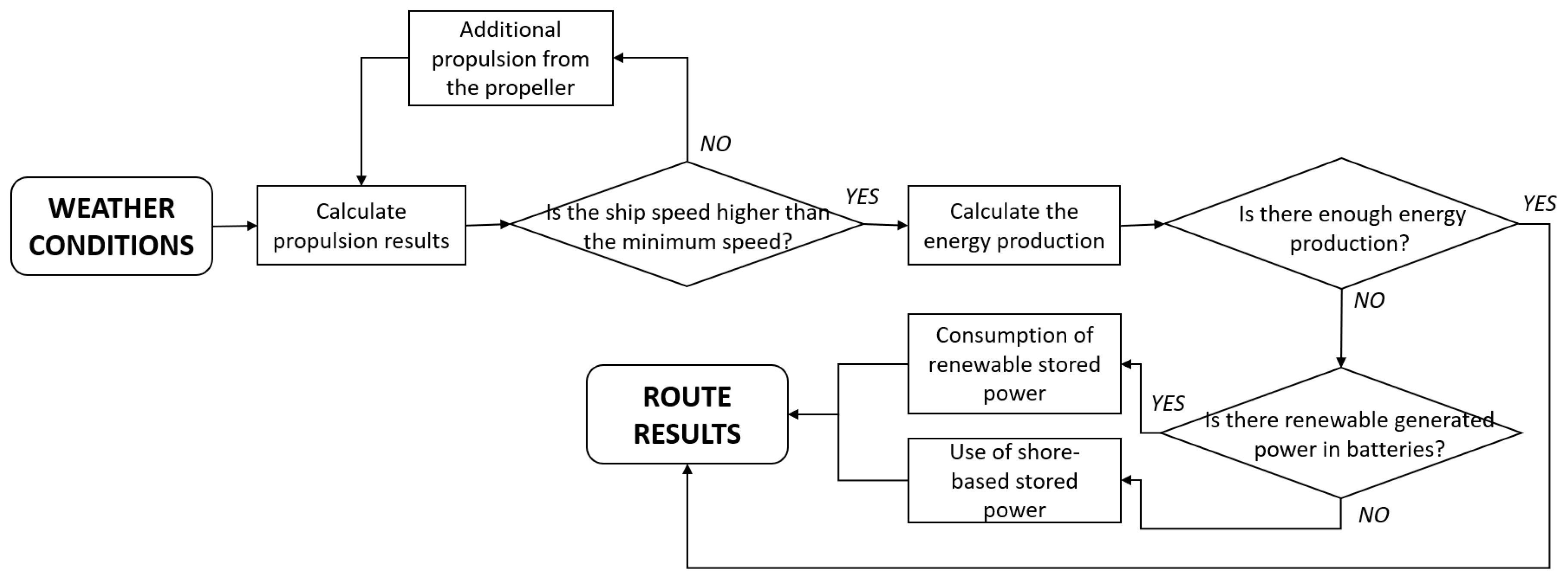With the same weather parameters, the power generation from wind turbines, solar panels, and a dual-mode propeller/hydro turbine in hydro turbines mode was calculated (see Section 2.2). To facilitate certain control of the speed during the journey, a parameter to limit the ship’s minimum speed was introduced in the model. If the attained ship speed in pure sailing mode was lower than the minimum speed, the hydro turbine turned to propeller mode to provide the additional thrust to achieve the minimum speed, using energy stored in batteries (see Section 2.1 and Section 2.2). The method focused on being open and generic to facilitate future modifications of routes and weather characteristics. The simulation procedure is presented in Figure 1.

2.1. Propulsion Systems

In this section, two wind propulsion systems (wing sails and Flettner rotors) are compared and evaluated. The VPP model ShipCLEAN was used to evaluate the main propulsion system, and a dual-mode propeller/hydro turbine was introduced as a support propulsion system while using propeller mode.

2.1.1. Flettner Rotors Versus Wing Sails

To select the most adequate wind propulsion system, it was required to compare the most feasible technologies currently available in the market. In this study, Flettner rotors and wing sails were compared. Both systems have pros and cons. This section motivates the selection of the most effective system according to the requirements of the concept ship.

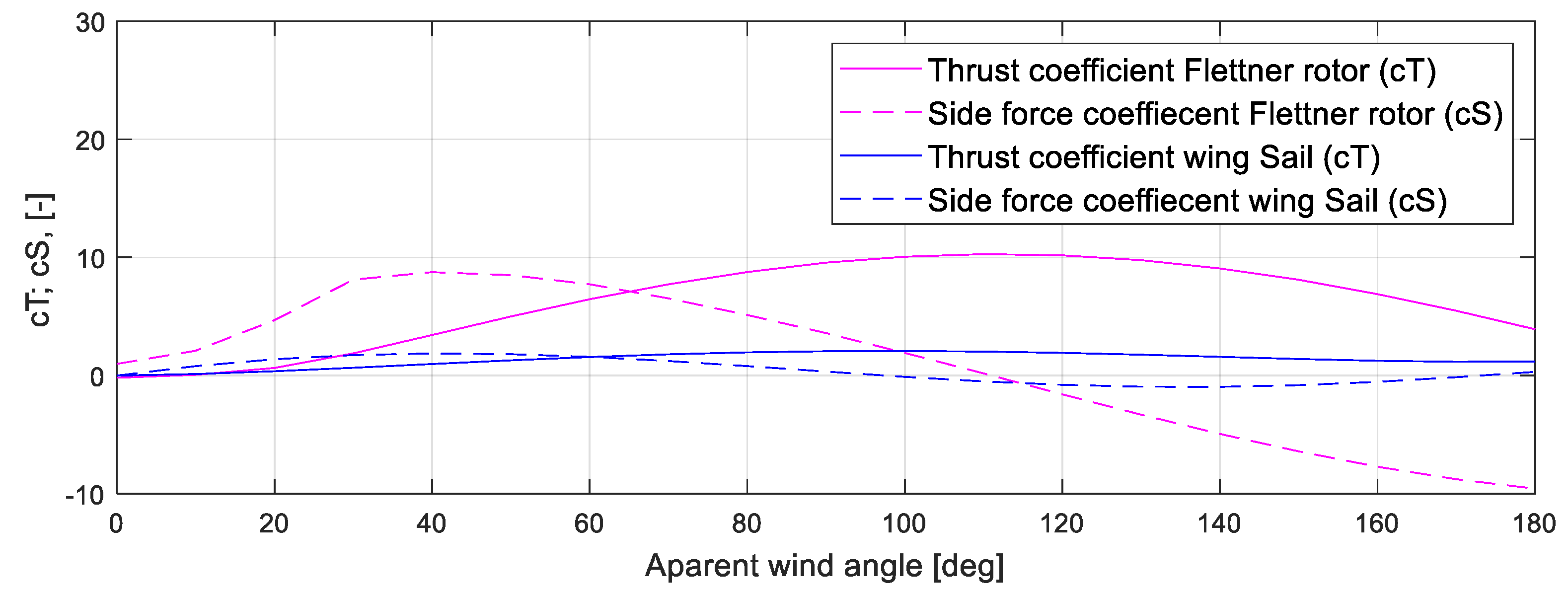
Thrust and side force coefficients ($C_{\left(t\right)}$ and $C_{\left(s\right)}$ respectively) are the parameters required to evaluate the forces generated by the sails. These parameters were used in Equations (1) and (2) to calculate the thrust and the side force of the ship ($F_{\left(x\right)}$ and $F_{\left(y\right)},$ respectively).

$$F_{\left(x\right)}=C_{\left(t\right)}\times A\times n\times \frac{\rho }{2}\times aw{s}^2$$

(1)

$$F_{\left(y\right)}=C_{\left(s\right)}\times A\times n\times \frac{\rho }{2}\times aw{s}^2$$

(2)

where $A$ is the sail area, $n$ is the number of sails, $\rho$ is the density of the air, and $aws$ is the apparent wind speed.

Figure 2 shows the value of the coefficients as a function of the apparent wind angle for a standard wing sail and a Flettner rotor. It was shown that the Flettner rotor produces higher forces in most of the conditions. This means that a wing sail always requires more sail area to generate the same thrust power (note that the sail area is the projected area of the cylinder or the sail).

The effect that these forces are producing when deciding to use Flettner rotors or wing sails in the concept ship is the resultant effect in sailing equilibrium. In both cases, the thrust force follows a similar pattern despite the higher values of rotors, with no production on for front winds, a peak in the range between 90°–130°, and a considerable reduction for back winds. However, the change in sailing behavior for the different systems is driven by the side forces.

In the case of wing sails, the side force appeared on the first range of speeds. From 0° to 55°, the side forces are higher than thrust. Therefore, in this period, the ship gradually started the movement with prominent drift. After 55°, the thrust increased while the side force started decreasing, achieving at 90°–110° maximum thrust with lateral force close to 0, this being the best condition for navigation. In the following range (110°–140°), the lateral force increased, but in a lower volume than thrust, so the drift was reduced. Finally, in the last section up to back winds, the thrust was reduced, and the lateral force was cancelled so that the drift was zero.

In the case where Flettner rotors were installed, in the first angles up to 65°, the side force was higher than the thrust with a starting of the movement with strong drift. After this critical point, the thrust force increased while the lateral force decreased, reaching the most optimal point at 110° when the thrust was maximum, and the lateral force was zero (condition where there is no drift). Finally, in the wind range from 110° to 180°, the lateral force increased while the thrust decreased, creating a situation for back winds with prominent drift and reduced thrust.

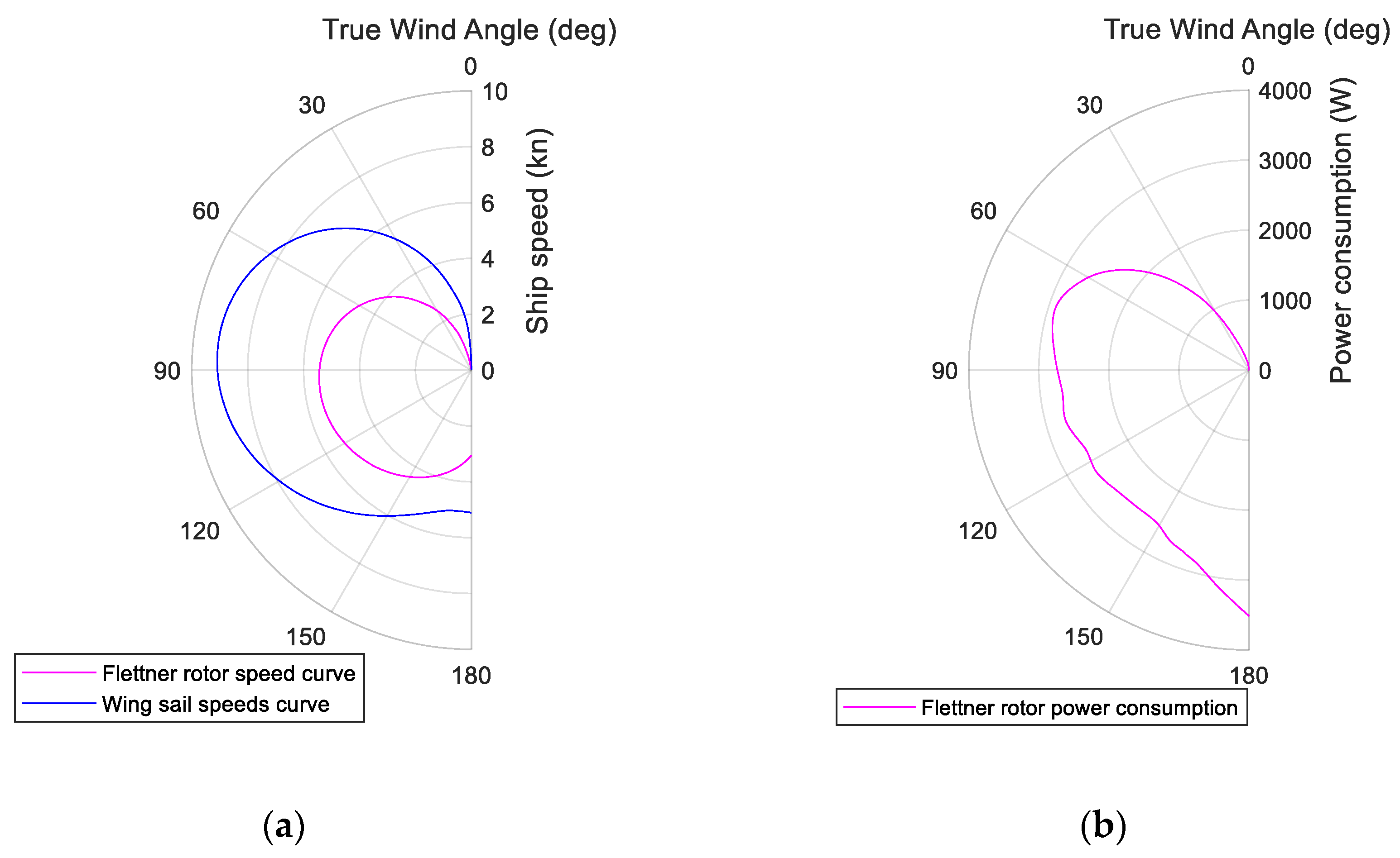
The effect of the thrust and side force was further evaluated with the speed calculation of the two different systems on an example vessel. Figure 3a shows a polar plot of the ship speed produced by one wing sail of 1800 m² of sail area (blue line) and a Flettner rotor of 150 m² of sail area (pink line) when the sails are individually installed in a high blockage hull with a length of 183 m [14]. The polar plot was produced using the VPP model ShipCLEAN, with an optimization of the rpm/angle of attack of the Flettner rotor and wing sail to achieve the highest possible ship speed. It was shown that with a Flettner rotor, the ship experienced significant decreasing in front and back winds. Instead, wing sails showed a more constant pattern for back winds.

Figure 3b shows the pattern of power consumption of the same example Flettner rotor. It is remarkable that in those angles where there is an extreme side force (50° and 180°), the consumption rose drastically to reach the optimum rotational speed.

Achieved speeds from Figure 3 show that for the two evaluated sails there was a higher thrust from a single wing sail than for a single Flettner rotor. However, from a practical point of view the sail area of the wing sail is twelve times bigger than the Flettner rotor; thus, the comparison is not determinant. Further research from [16] simulated two different routes for a tanker ship and compared the fuel savings when Flettner rotors or wing sails were installed onboard as wind-assisted propulsion systems. The result of the study showed that fuel savings using Flettner rotors are slightly higher than using wing sails (0.1–0.4% higher), even considering the power required to spin the rotors.

To evaluate and motivate the most suitable wind propulsion technology for the project, other factors than the achievable ship speed must be considered. From a practical point of view, autonomous control of the system is essential. Flettner rotors are easier to operate as the rotational speed is the only parameter that needs to be adjusted for maximum efficiency; cf. [14,17]. It is also necessary to reduce negative interactions of the sail with other renewable systems. Due to the smaller required sail area, Flettner rotors are more suitable to save space and reduce negative interaction with other systems, e.g., solar panels ([14,18]).

Flettner rotors have been selected in the study as the main propulsion system for their high efficiency in real environmental conditions, their flexibility and simplicity in operation, and their small sail area that reduces their interference with other renewable technologies on deck. Additionally, the ShipCLEAN model has already been validated proving reliable results using Flettner rotors as a wind-assisted propulsion system [15].

2.1.2. The ShipCLEAN Model

ShipCLEAN is a ship performance prediction model developed to estimate the energy consumption of a vessel based on a limited number of required inputs. The design of the model has an open format to enable simulations for different ship types and weather conditions. It was developed and prepared for the possibility to include wind-assisted propulsion to present the positive influence that wind energy can have in the maritime market, see [18] for detailed information. In the current study, the model was used to evaluate the performance of a ship with wind power as the main propulsion system.

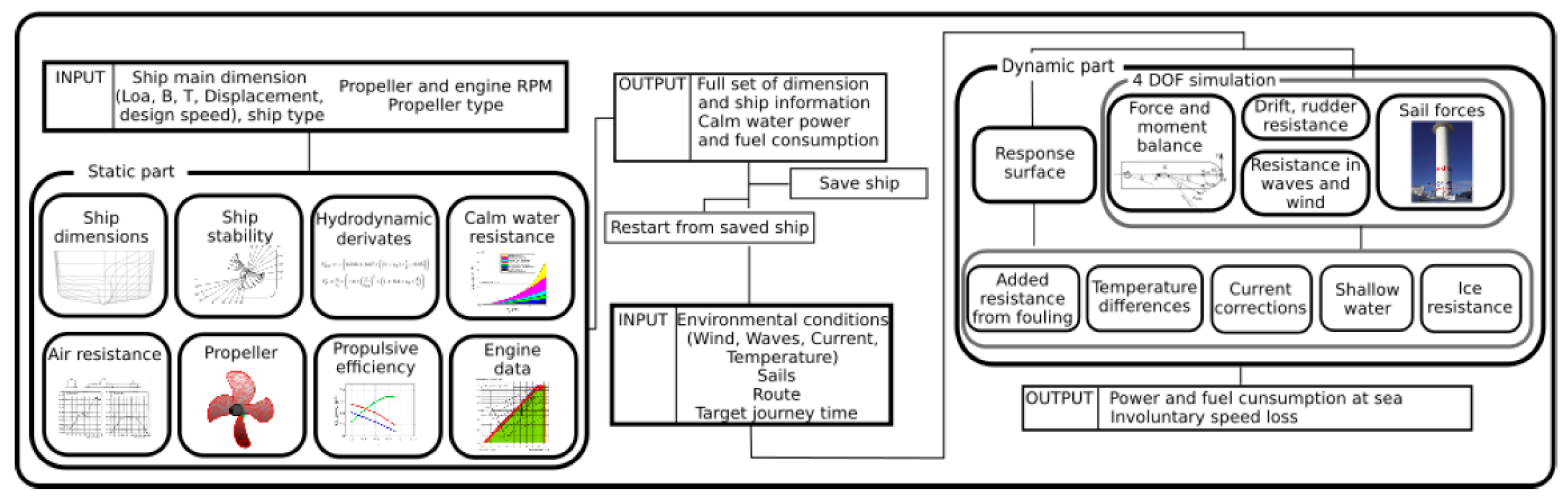
To predict the ship’s performance, the model is designed to follow the process in Figure 4. ShipCLEAN requires some static inputs, i.e., ship design characteristics (main dimensions, design speed, ship type, and propeller dimensions), dynamic inputs as the weather parameters (wind speed and direction, currents and water temperature), and wind technology characteristics (sail area, number of sails, thrust coefficient, and side coefficient).

The static part of the model uses empirical formulations to convert the basic ship dimensions into a set of detailed parameters that define hull shape, stability, and resistance (calm water resistance and air resistance). Results from the static part are then used for the dynamic analysis where, together with the weather characteristics and the sail system dimensions, a balance of applied forces is evaluated for 4 degrees of freedom (DOF). According to [17], the analysis for 4 DOF (surge, sway, yaw, and heel) in the balance of forces is a requirement when using wind power propulsion in a ship. For this type of analysis, the forces and moments that take place are divided into aerodynamic (mainly consistent in the wind-assisted system but also other structures above the waterline) and hydrodynamic (underwater structures such as the hull and rudder are analyzed against the water flow). The center of forces is then defined as the point where lift and drag are applied. As the aerodynamic and hydrodynamic forces have their center of forces in a different longitudinal point of the ship, a yaw moment is generated, which must be compensated by the rudder.

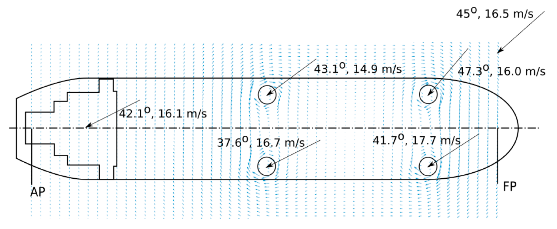
The method used in ShipCLEAN to simulate the behavior of Flettner rotors has been designed to give highly accurate results. Interaction effects between sails and other elements of the vessel have relevant attention on the simulation model design. Aerodynamic interaction effects are modelled considering the influence of multiple rotors on the ship, and the vertical wind speed distribution is simulated. The optimal rpm of the rotors is found by optimizing the individual rpm for best performance considering power consumption and added resistance from drift and rudder. The induced speeds and resulting local wind speeds and angles for a ship with four rotors are shown in Figure 5. Additionally, a parameter defining the maximum allowed power consumption of the rotors is introduced. In this case, the conditions were re-optimized; see [15,17] for details. In the current study, ShipCLEAN was used to predict ship speed and Flettner rotor power consumption, respecting 4 DOF.

2.1.3. Dual-Mode Propeller/Hydro Turbine (Propeller Mode)

The dual-mode propeller/hydro turbine is ideated as a system that, in propeller mode, generates thrust when sail propulsion does not provide enough thrust to achieve the minimum ship speed. In conditions when the propeller mode is not required, it can make use of the water flow through the blades to generate electricity as a hydro turbine. Considering these operational conditions, the hydro turbine is always working in the highest range of ship speeds, while the propeller mode is used in the lowest range of speeds to reach the minimum required ship speed.

The system, not common yet in the market, has been previously studied and simulated in [11] as an efficient energy source for wind propelled ships. The study evaluated three different propellers with different pitch ratios. In all cases, it was shown that, even for low speeds, the system produced high power showing technical viability.

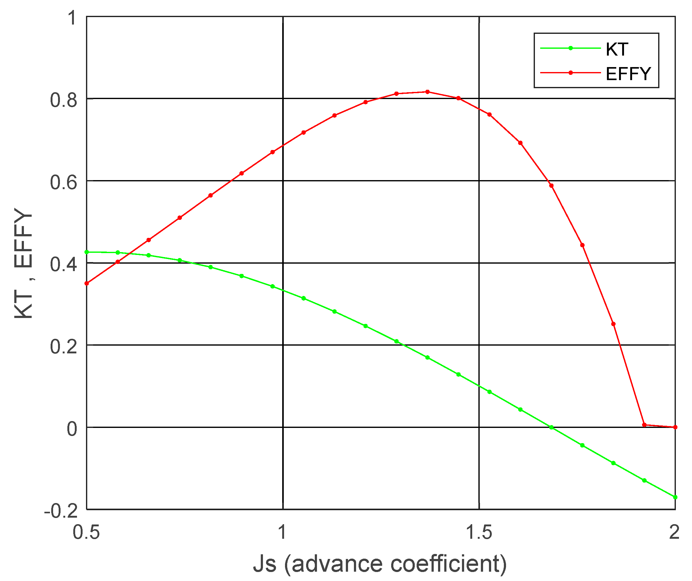
The design of this propeller with double functionality is a challenge, as it must work in both propeller and turbine mode. The propeller was designed using the Matlab open-source code “OpenProp” [19] by optimizing a profile “NACA 65A010”. The parameters that have been evaluated in the process were the camber, the ship speed design, and the design RPMs of the propeller. The rest of the parameters were optimized automatically for each case. The optimization was done to have a good relation of power coefficient and drag coefficient for hydro turbine mode and a maximum peak of propeller efficiency for propeller mode. For the calculation of the thrust in propeller mode, propeller curves were obtained from “OpenProp”. The curves required were the thrust coefficient (KT) and the efficiency (EFFY) of the propeller shown in Figure 6.

The calculation of the power consumption of the propeller to reach the minimum speed defined was evaluated with Equation (3) [11]:

$$P_{prop}=\Delta T{v}_{ship}{\eta }_{prop}{\eta }_{mot}$$

(3)

where $\Delta T$ is the increment of thrust needed to reach the minimum required speed, $v_{min}$, $v_{ship}$ is the speed reached by the ship making use of the propeller (corresponding to $v_{min}$), ${\eta }_{prop}$ is the propeller efficiency from OpenProp curves, and ${\eta }_{mot}$ is the efficiency of the electric motor set as a constant value of 95% [11,20].

2.1.4. Speed Limit and Velocity Made Good (VMG)

The speed limit was introduced into the simulation model to control the sailing performance on a route. The limitation is defined by a minimum speed ($v_{min}$). If the pure sailing propulsion does not give enough thrust to reach $v_{min}$, the dual-mode propeller/hydro turbine will provide additional thrust.

The performance of wind propulsion is highly dependent on the wind angle and speed. Thus, wind-powered vessels require an adapted trip plan, depending on the wind characteristics. The adaptation was done by the velocity made good (VMG) optimization function. This function avoids conditions where no wind thrust is produced and optimizes the deviation angles (tacks) for maximum speed towards the target. Under regular, pure wind propulsion conditions, the VMG function evaluated the Flettner rotor performance and ship resistance from ShipCLEAN for different deviation angles from the direct course. The optimal condition was obtained as the maximum VMG by processing the ship speeds and deviation angles, see [14] for details.

In conditions where the total thrust is partly produced by the propeller (because $v_{min}$ cannot be reached with pure sailing), the optimization function calculated the angle that requires the lowest energy consumption to reach a VMG equal to $v_{min}$. $v_{min}$ is always considered in the VMG function. This means that although the real ship speed accomplishes the limit, VMG is the speed that needs to be above the limit considering the deviation angles.

2.2. Power Energy System

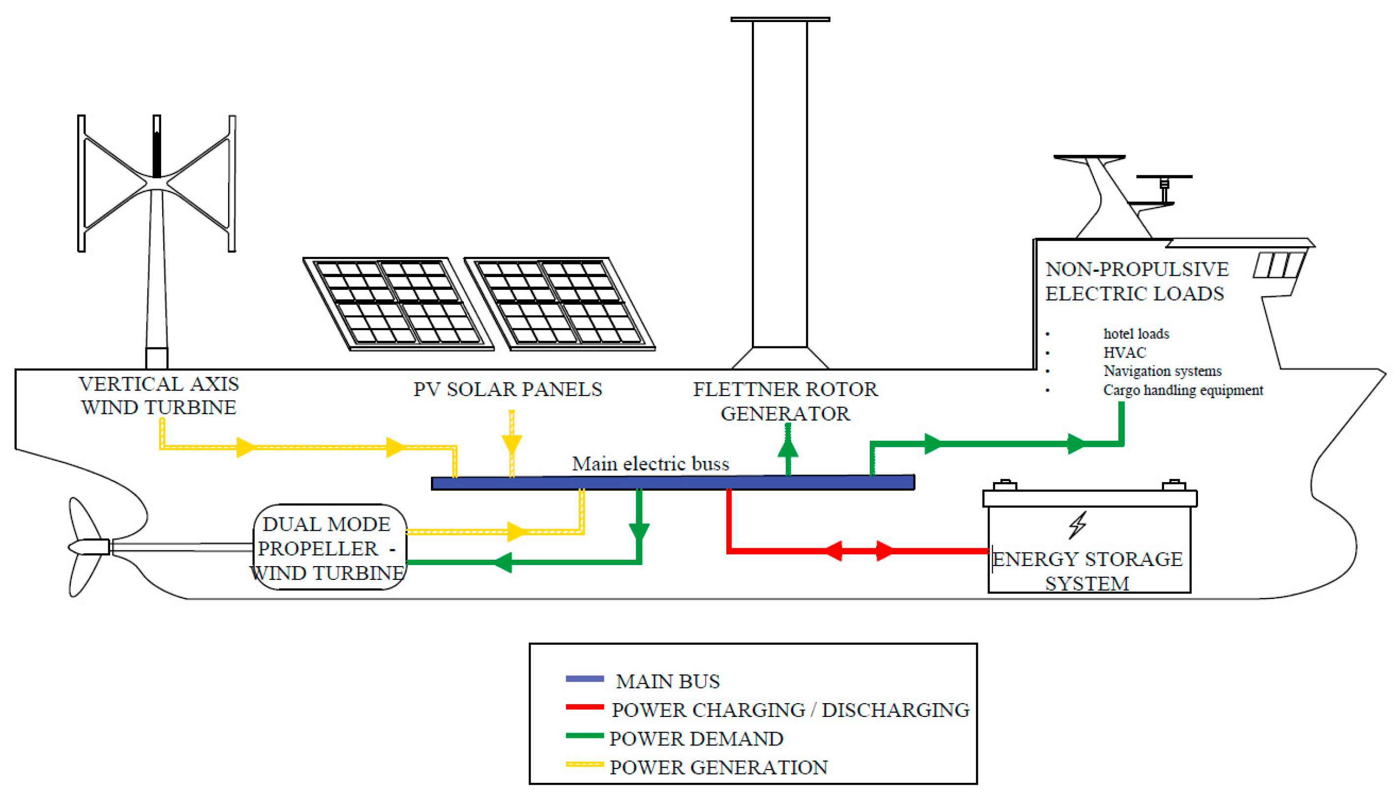
A challenging aspect of the study is the generation of energy onboard. The configuration of renewable technologies must be optimal for maximum energy production. In the former study [14], the strength and disadvantages of some of the most developed renewable systems in the market were shown. A basic diagram of the systems energy flow considered in this study is shown in Figure 7. The figure shows the energetical connections of the system. The electrical consumers are divided into two groups, the propulsion systems and the non-propulsive systems. The first group is explained in Section 2.1. The non-propulsive systems group compromises all the additional consumers to operate the ship, like machinery, governance, navigation, communication, and habitability. The electric producers evaluated were the renewable systems installed onboard. The considered systems were vertical axis wind turbines, PV solar panels, and the turbine mode of the dual-mode propeller-hydro turbine, all of them highly dependent on weather conditions. Finally, to balance the power in those conditions where there is a surplus or insufficient power, the concept was supported by a battery storage system. This section presents a summary of the electric producers and battery systems and how they were implemented and coupled with ShipCLEAN.

2.2.1. Wind Turbine

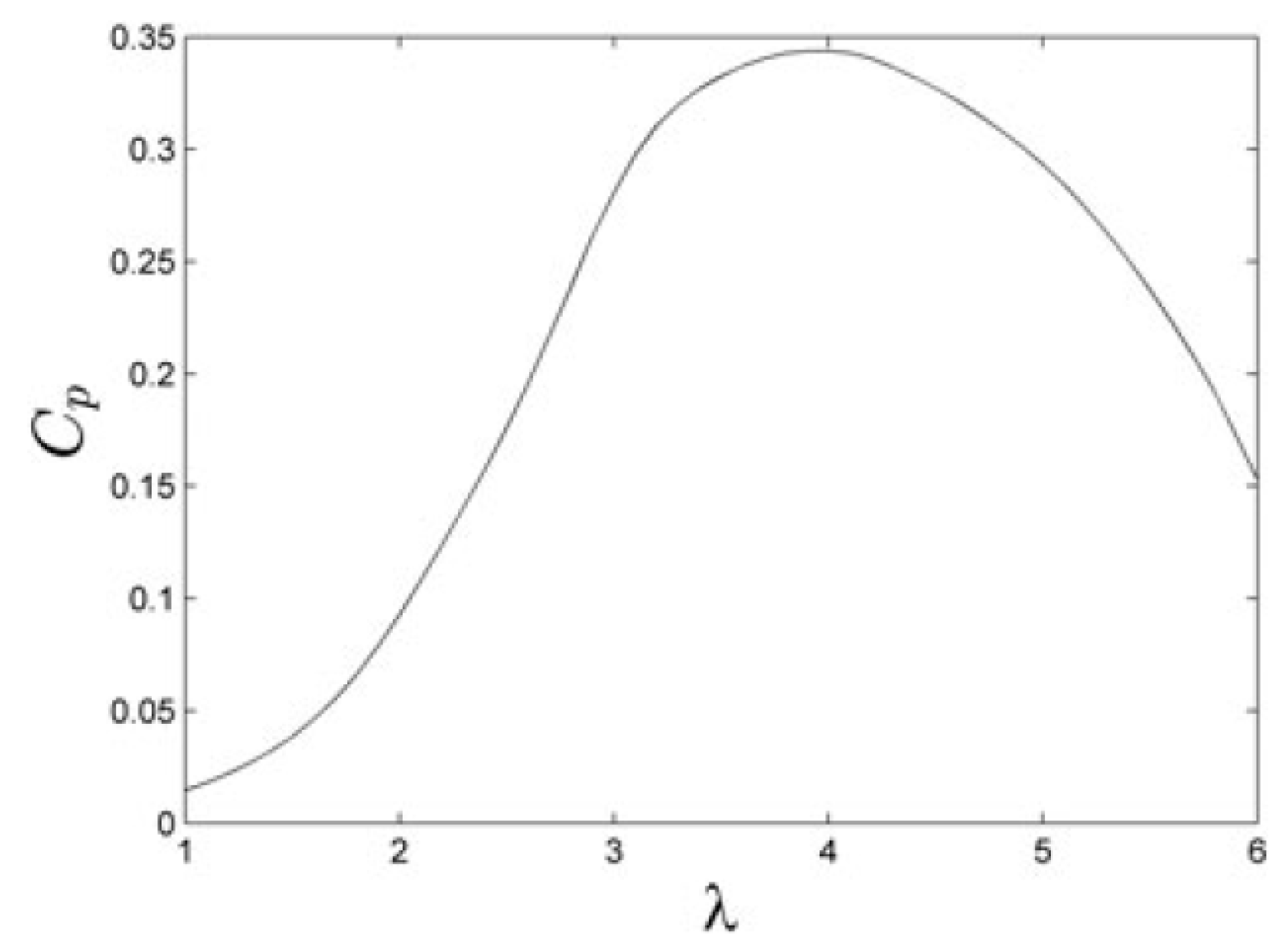
The vertical axis wind turbine was motivated due to its stability and functionality reasons, see [14] for details. The system has the function to generate electrical energy from the wind, which is used directly or stored in batteries. The wind turbine model assumes conditions of constant wind speed and direction for a fixed period, then, energy production is constant. The power generated by the wind turbine was calculated according to Equation (4):

$$P_{wind}=0.5C{p}_{wind}{\rho }_{air}{\eta }_{wind}{A}_{wind}{v}_{wind}{}^3$$

(4)

where $C{p}_{wind}$ is the power coefficient from [21] shown in Figure 8, a factor that determines the conversion efficiency from the wind to the electrical generator. ${\rho }_{air}$ is the density of the air, and ${\eta }_{wind}$ is the efficiency of the generator (assumed in [21] as 85%). $A_{wind}$ is the area of the turbine, i.e., the length of the blades multiplied by the diameter of the rotor, and $v_{wind}$ is the wind speed.

The wind turbine has three reference speeds: minimum, nominal, and a cut-off speed. The minimum speed corresponds to the minimum wind speed required for the generator to start producing energy. Once the generator surpasses this limit, it increases its production until the wind speed is equal to the nominal wind speed where the production efficiency is maximum (from Figure 8, λ ≈ 4). Above the nominal speed, the rotational speed is maintained with the same power coefficient and a constant energy generation. When the wind reaches the cut-off speed, the turbine stops for safety reasons, and energy production becomes zero. The current numerical model does not consider the drag force generated by the turbine, as it is assumed to have a low impact considering the total ship resistance and forces generated by the Flettner rotors [8].

2.2.2. Solar Panels

Solar panels were placed on the weather deck of the concept ship covering the free available area. Photovoltaic installation is a system that requires an extensive open area to generate the amount of power demanded by a vessel. As is discussed in the assumptions from Section 2, a ship that requires the open deck to handle the cargo is not considered in the present study. It is assumed that the placement of the panels does not interfere with the ship operation or other systems onboard. The energy production of the solar panels was calculated using Equation (5); see [10,22,23].

$$P_{PV\left(t\right)}={\eta }_{pv}{A}_{pv}{I}_{\left(t\right)}$$

(5)

where $I_{\left(t\right)}$ is the solar radiation intensity, $A_{pv}$ is the area of the solar panels, and ${\eta }_{pv}$ is the efficiency for different generation parameters. The efficiency ${\eta }_{pv}$ is defined by Equation (6):

$${\eta }_{pv}={\eta }_{ref}\left(1-\beta \left(T_c-T_{ref}\right)\right){\eta }_{conv}$$

(6)

where ${\eta }_{ref}$ is the reference efficiency determined by the manufacturer, $\beta$ is the temperature coefficient of the cell material, $T_{ref}$ is the cell reference temperature, $T_c$ is the photovoltaic (PV) cell temperature, and ${\eta }_{conv}$ refers to other conversion loses from radiation to electric energy independent of the installation. The losses considered for solar panels with regular leaning and maintenance are the module degradation loss of 1%, dust and salt losses of 2%, reflection loses of 2.5%, and other electrical losses of 4% from the panel to the main bus of the grid [24,25]. Note that the current model does not account for shadow losses.$A_{pv}$ is the area of the PV surface defined in Equation (7). It is defined as the number of panels, $n$, multiplied by the area of each panel, $A_{panel}$.

$$A_{pv}=n{A}_{panel}$$

(7)

The solar radiation intensity, $I_{\left(t\right)}$, received by the photovoltaic panel surface was calculated according to Equation (8). The parameter $I_{B,N}$ denotes the direct radiation perpendicular to the surface defined by the weather data. $\theta$ is the angle between the board and the solar rays, $\varphi$ is the tilt angle from the horizontal surface, $\chi$ is the zenith angle or angle between the sun, and the vertical and $\rho$ is the Albedo or reflection index ([10,23]).

$$I_{\left(t\right)}=I_{B,N}(\cos \left(\theta \right)+co{s}^2\left(\frac{\varphi }{2}\right)\sin \left(\chi \right)+\rho \cos \left(\chi \right)si{n}^2\left(\frac{\varphi }{2}\right))$$

(8)

2.2.3. Dual-Mode Propeller/Hydro Turbine (Hydro Turbine)

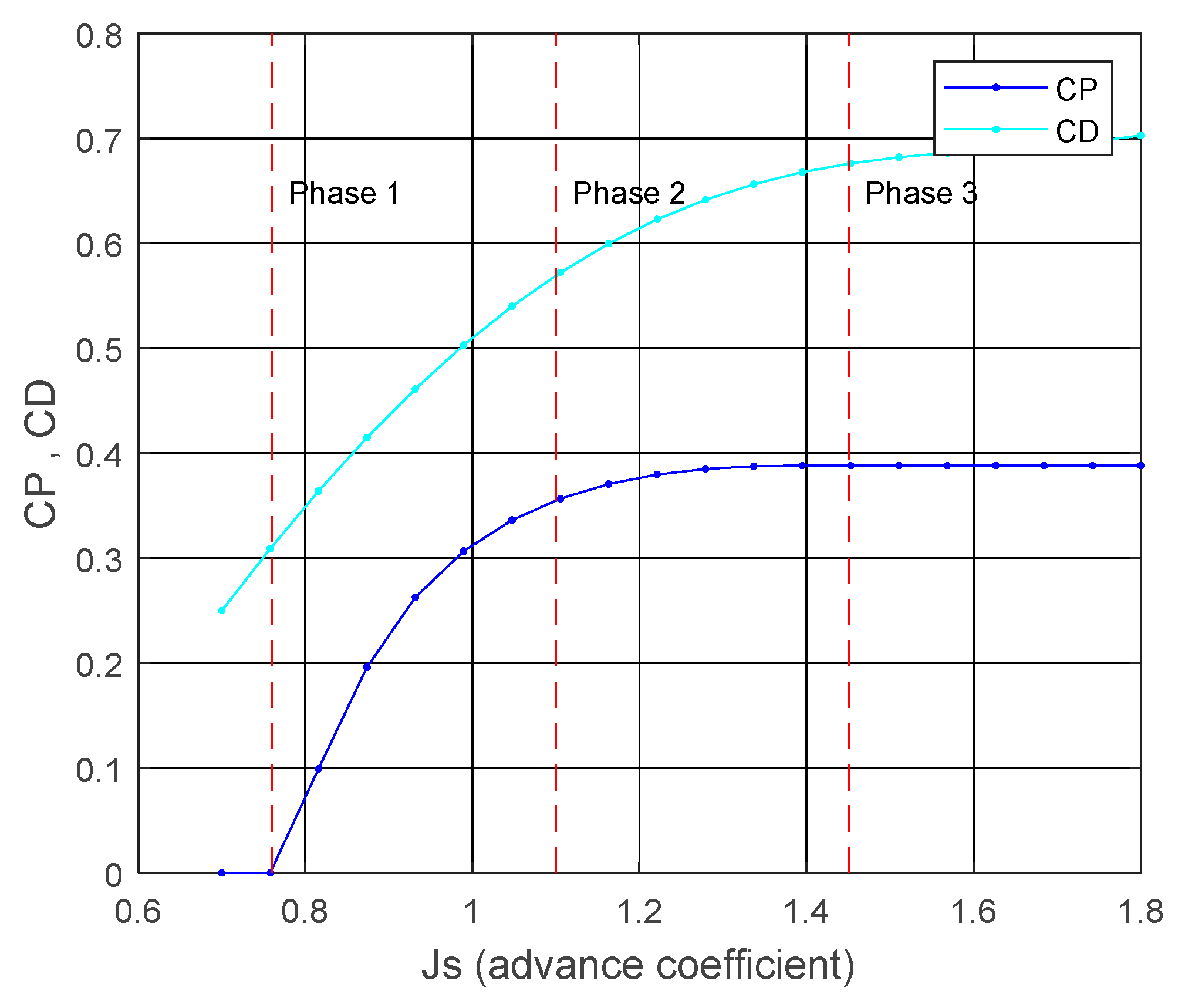
Numerical calculations of the propeller-hydro turbine system were evaluated from the results obtained in the open code “OpenProp” [18]. The simulation of the hydro turbine generation system required from “Open Prop” the turbine curves of the drag coefficient ($CD$) and power coefficient ($C{P}_{H/T}$) shown in Figure 9. The curves were used to calculate the power generation and drag force of the propeller by using the Equations (9) and (10):

$$P=\frac{1}{2}C{P}_{H/T}{\rho }_{water}{A}_{prop}{v}_{ship}{}^3{\eta }_{H/T}$$

(9)

$$F_{drag}=0.5CD{\rho }_{water}{v}_{ship}{}^2{A}_{prop}$$

(10)

where ${\rho }_{water}$ is the water density, $A_{prop}$ is the circular propeller area, $v_{ship}$ is the ship velocity, and ${\eta }_{H/T}$ are the efficiencies of the gearbox and the generator, set to 89% [11,26].

The hydro turbine function starts working when the ship speed produced with wind propulsion reaches the minimum allowed speed. At this point, the power supply to the propeller stops, and the propeller starts a free rotating movement caused by the water flow through the blades. The free rotation is referred to the lowest value of drag coefficient, but as the torque from the electric generator is not applied, CD is zero, and the generation of electric power is zero (as a reference, this point is defined in Figure 9 as Phase 1). From the first condition, if the thrust from the sails increases, torque to the generator is applied, reducing the rotational speed of the propeller and increasing its advance coefficient (J) that results in a higher CP and CD that maintain the ship to the minimum ship speed and increase the power production (defined as Phase 2 in Figure 9). The advance coefficient increases with the sails’ thrust to the point where CP reaches its maximum. Then CD and CP stay stable independently of the thrust. In this condition, the ship speed increases with the maximum power coefficient (represented as Phase 3 in Figure 9).

2.2.4. Batteries

In the concept ship model, battery functions control the energy distribution around the ship by storing the surplus of the energy generation or by supplying energy to the ship consumers when not enough power is produced. If the global power balance is positive, the charging battery function is activated. With this mode, the system first stores the energy from DC producers as PV panels, and afterwards, the AC generators as hydro turbines and wind turbines as it optimizes the electric conversions. For this system, charging efficiency of 85% was assumed [27].

The discharging battery function is used when the power balance is negative. For this case, if the ship speed is higher than the minimum velocity requirement, the model reduces the delivered power for the Flettner rotors adapting the ship speed to $v_{min}$. If the ship reaches $v_{min}$ and the power balance is still negative, the discharging battery function uses the energy stored in the batteries to fulfil the demand. For the energy discharging from the batteries, the efficiency is assumed to be 85% [27].

If additional energy is required, and all the energy produced by renewable systems and stored is already used, additional energy is required to fulfil the demand. It was assumed that shore-based electricity is stored in the batteries before the start of the trip. It was also assumed that there are always enough batteries in the ship. The resulting energy balance from route simulations defines the necessary number of batteries.

2.3. Environmental Conditions

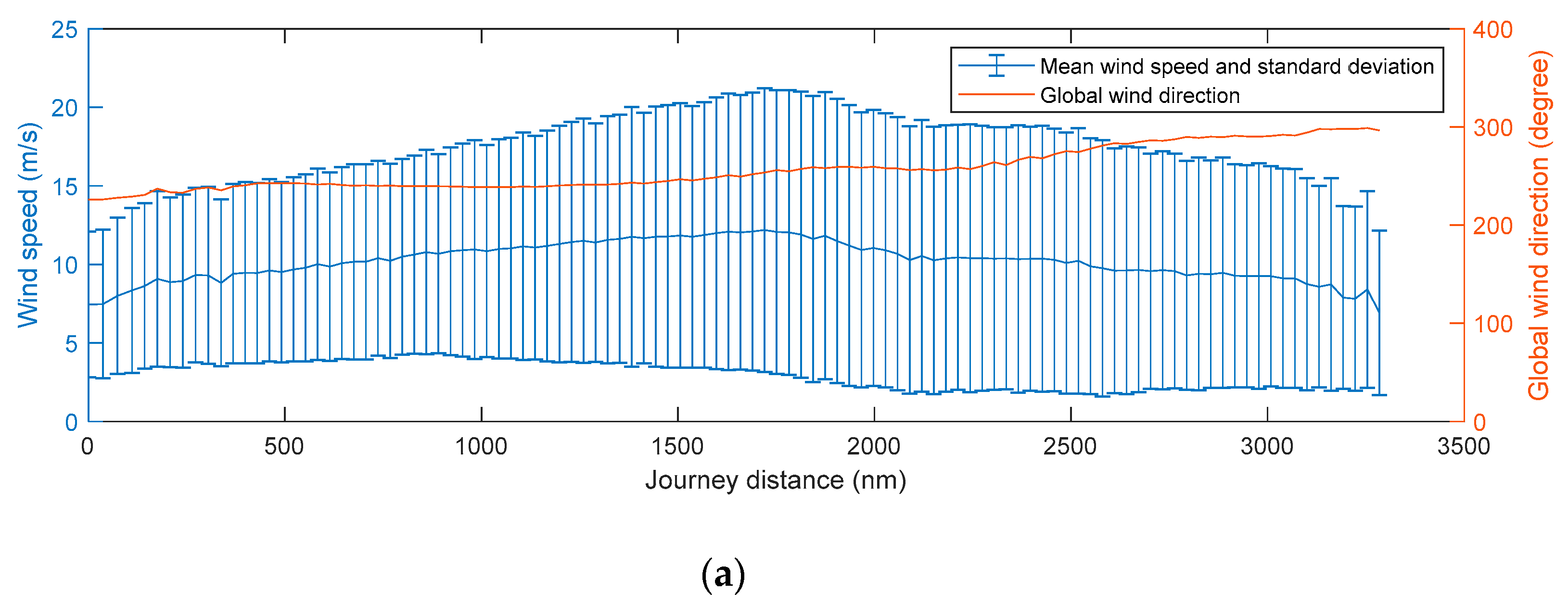
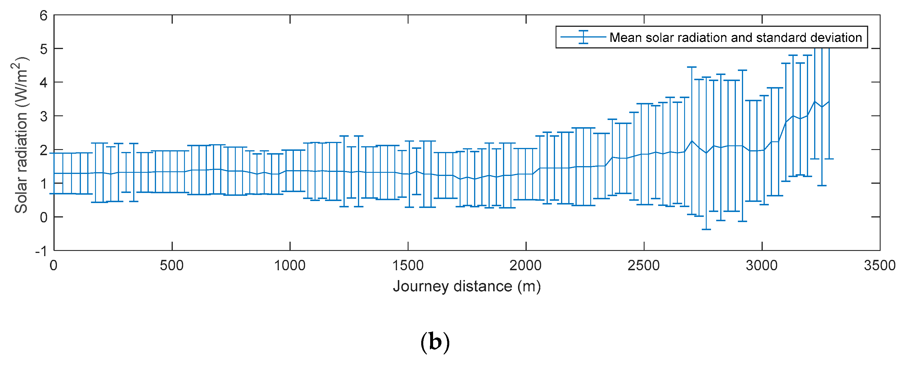
An accurate definition of the weather condition is essential to estimate realistic ship behavior and trustable results. The process to generate the environmental conditions starts from average weather data source provided by [28]. It is based on global historical data from 1983 to the present. It is defined in a grid of 0.5 × 0.5 degrees covering all of the surface of the planet, and it gives the result for each month of the year. Within this data source, it is defined as the mean value and the variance of wind speed and direction, solar radiation, and temperature.

To mimic realistic weather conditions, the average data must be converted to include variation in time, although the continuous variation would create an infinite number of calculations. The most practical and accurate way to deal with this is to define a period when the weather variables are assumed to be constant. In this study, it was set as one hour.

For each period, the weather values changes. The mean and variance of each weather parameter were used in Monte Carlo simulations to generate random weather variables assuming Weibull distributions for the wind speed and Normal distributions for the wind angle, solar radiation and temperature. As this process was done to obtain the time at sea, and uncertainties in weather data are crucial for the results, a total of 100 random values for each weather variable were generated.

The process starts when the ship enters a square of the grid and average data is defined, the random values are generated, and the simulation calculates results for the sequence of random values with the time advance. When the ship reaches the end of a square, new random values are generated with the new average data. This process is continued until the end of the voyage.

2.4. Concept Ship

2.4.1. Ship Characteristics

The 183 m length high blockage ship (with block coefficient of 0.80) previously studied in [14] was used in this study. The ship characteristics are defined in

Table 1. Concept ship dimensions.

Ship Dimension	Value
LOA (Length Overall)	183 m
Draft	11 m
Breadth	32.2 m
Displacement	50,618 t
Renewable systems weight	1050–1520 t
Block coefficient	0.80

.

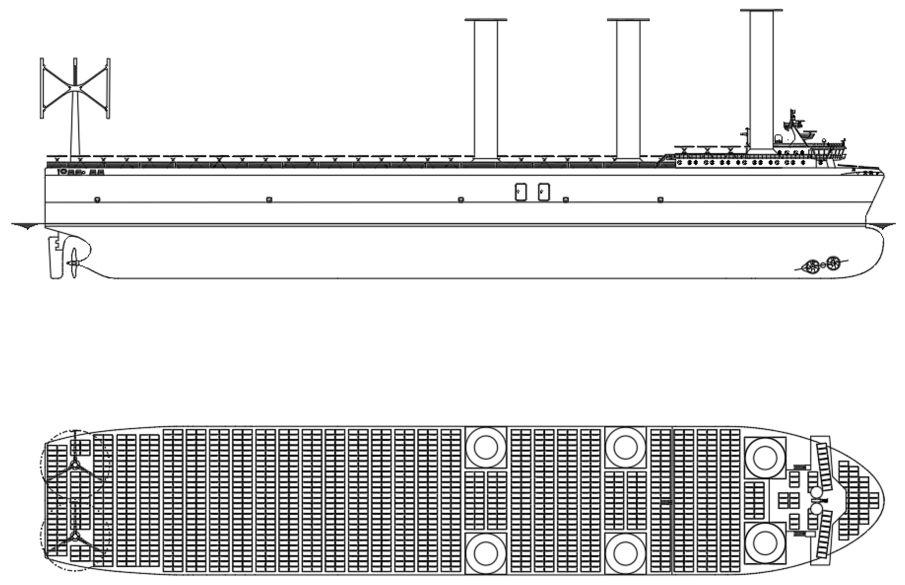
The vessel is equipped with six Flettner rotors (5 × 30 m), a dual-mode propeller/hydro turbine, two vertical axis wind turbines, and 1564 solar panels. A schematic of the concept ship with the system distribution is shown in Figure 10. The energy consumption for the propulsive systems was calculated with the simulation model, while the non-propulsive consumption was estimated from previous studies. According to [29], a ship with the previously mentioned characteristics during sailing condition has 153.9 kW power demand from machinery services, 11 kW power demand from governance service, 20 kW power demand from navigation assistance and communication service, and 41.9 kW power demand from habitability service. In total, it was considered that the power consumption while sailing is 226.8 kW. It was assumed that the power demand is constant during all the simulation. A weight evaluation was done to see the influence of renewable systems on ship loads. The total added weight on the ship is in the range between 1050 and 1520 tons, which corresponds to 2–3% of the total ship displacement [30,31,32]. Considering that the weight of the fossil fuel machinery and the fuel are removed, it is assumed that the weight increment produced can be easily balanced with cargo weight reduction.

2.4.2. Flettner Rotors

Six Flettner rotors are symmetrically positioned on both sides of the ship (three on each side). Each rotor is 30 m high and 5 m in diameter. The rotors are installed in the front of the ship to advance the center of forces. An advanced position of the rotors, and the high side forces of the Flettner systems, are proved to give the most adequate drift condition for the studied ship to maximize the range of wind angles that the ship is able to sail and to minimize the required rudder angle for each sailing condition [15]. The previous studies [14,15] demonstrated that the configuration established with the respective rotor dimension is the most beneficial, assuming the attained speeds and energetical efficiency as the most critical aspects.

2.4.3. Vertical Wind Turbine

Two vertical axis wind turbines with three 13 m long blades, a rotor diameter of 15 m, and a nominal power generation of 70 kW were installed. The reference wind speeds for the turbine are 3 m/s as the minimum wind speed, 12 m/s of nominal wind speed and 26 m/s cut-off speed; see [8,21].

2.4.4. Photovoltaic Solar Panels

Solar panels cover the whole weather deck. There is a total of 1780 solar panels with an area of 2.16 m², a nominal power of 460 W each, and a panel efficiency of 21.3%. The supporting structures for the panels were not considered, but it is assumed that these structures do not interfere with the crew operations.

2.4.5. Dual-Mode Propeller/Hydro Turbine

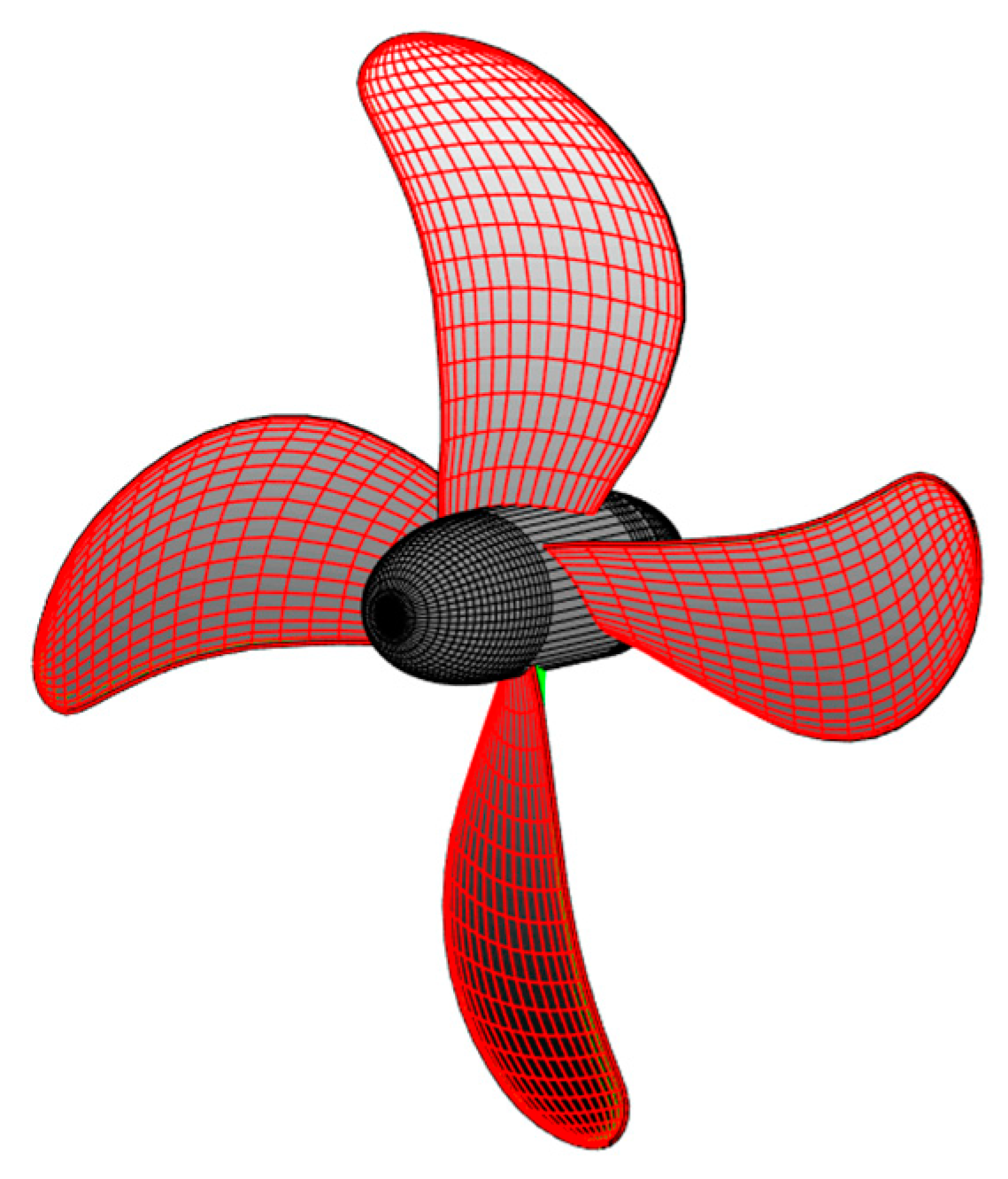
The system is composed of one propeller / hydro turbine with a diameter of 4 m and four blades. The propeller is designed for good performance in propeller mode below a $v_{min}$ of 5 knots speed and for good turbine mode above that speed. The optimization process gave as the optimum result a propeller without camber with its maximum efficiency rotating with an advance coefficient of 1.4. The propeller and turbine diagrams are shown in Figure 6 and Figure 9. A 3D model of the propeller used is shown in Figure 11.

3. Results

This section presents results from the numerical model, simulating the performance of the concept ship on routes under realistic weather conditions, intending to identify the optimal operation of the concept ship under varying conditions

Two different routes were evaluated: (A) a short distance route in the Mediterranean Sea between the ports of Barcelona (Spain) and Tunis (Tunisia) with a total distance of 496 nautical miles, starting on the first of January at 7 am, and (B) a transatlantic route from Rotterdam (The Netherlands) to New York (U.S.) with a total distance of 3284 nautical miles, starting on the first of January at 7 am. The selection of route A was motivated by the fact that: (i) a short route has lower variability in the weather during the route and lower safety margins are required, (ii) the Mediterranean sea is a good region for the photovoltaic generation with a high solar radiation prognostic [28], and (iii) the Mediterranean has mild weather conditions, creating a challenge for wind propulsion and energy technologies [28]. Route B was chosen as the opposite case of route A. It has a higher number of unpredictable conditions; therefore, it requires higher safety margins for energy consumption. The route in the Atlantic ocean faces rough weather conditions, which would produce higher speeds and energy production from the wind [28].

Two sailing conditions for each route have been defined depending on $v_{min}$. The conditions are limited speed cases when $v_{min}$ is 5 knots and open speed when there is no minimum speed. The objective was to find the most efficient performance between sailing with just the wind propulsion system or including propeller power to always achieve a minimum speed. The four study cases evaluated in the present study are:

• Case (i): Route Barcelona–Tunis with limited speed
• Case (ii): Route Barcelona–Tunis with open speed
• Case (iii): Route Rotterdam–New York with limited speed
• Case (vi): Route Rotterdam–New York with open speed

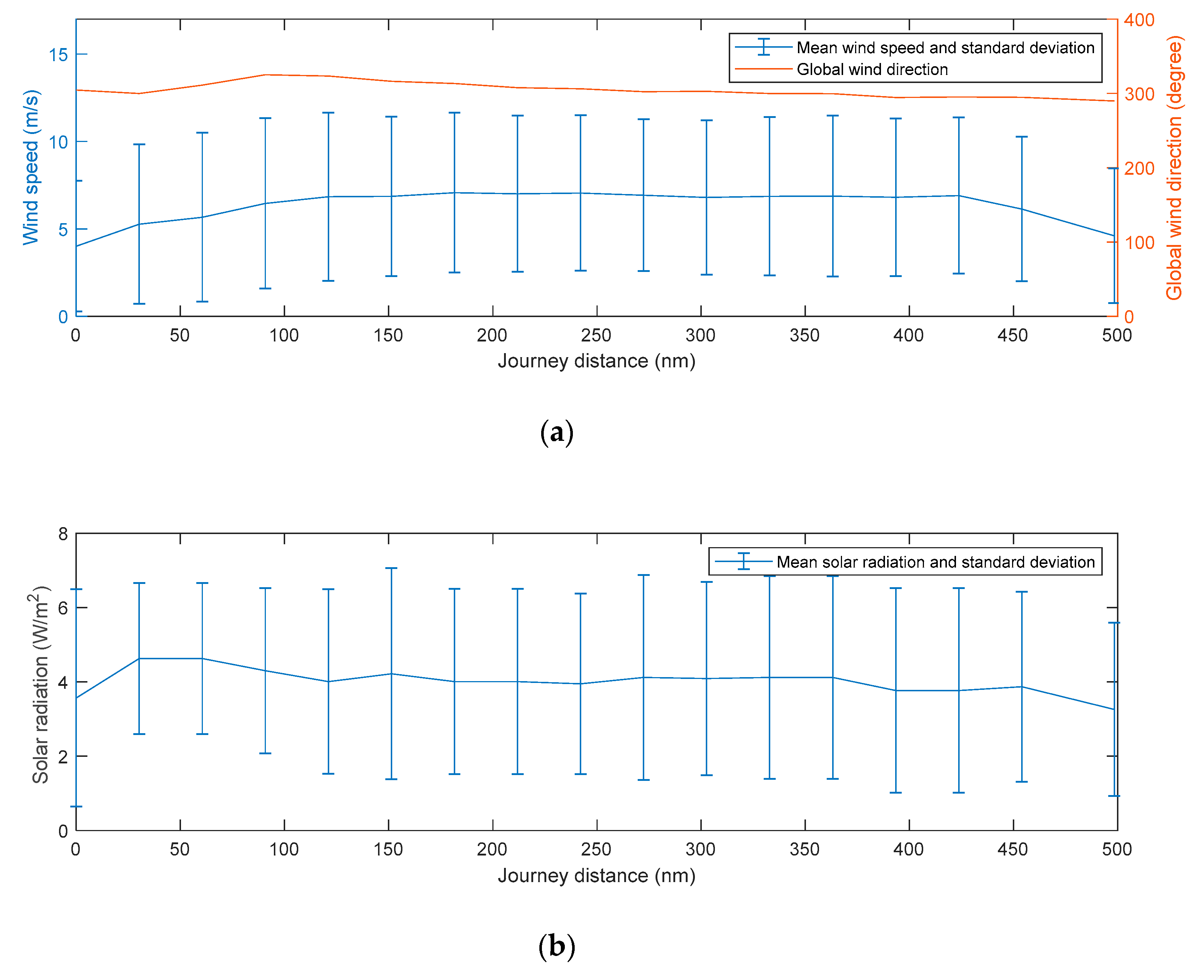
To simulate the long-term performance of the concept ship in realistic conditions, probability distributions were generated for the environmental conditions, i.e., the wind speed and directions as well as the solar radiation. For the current study, Monte Carlo simulations with 50 variants were simulated for each case. Figure 12 and Figure 13 present the weather statistics used to define the randomly distributed weather values for each route.

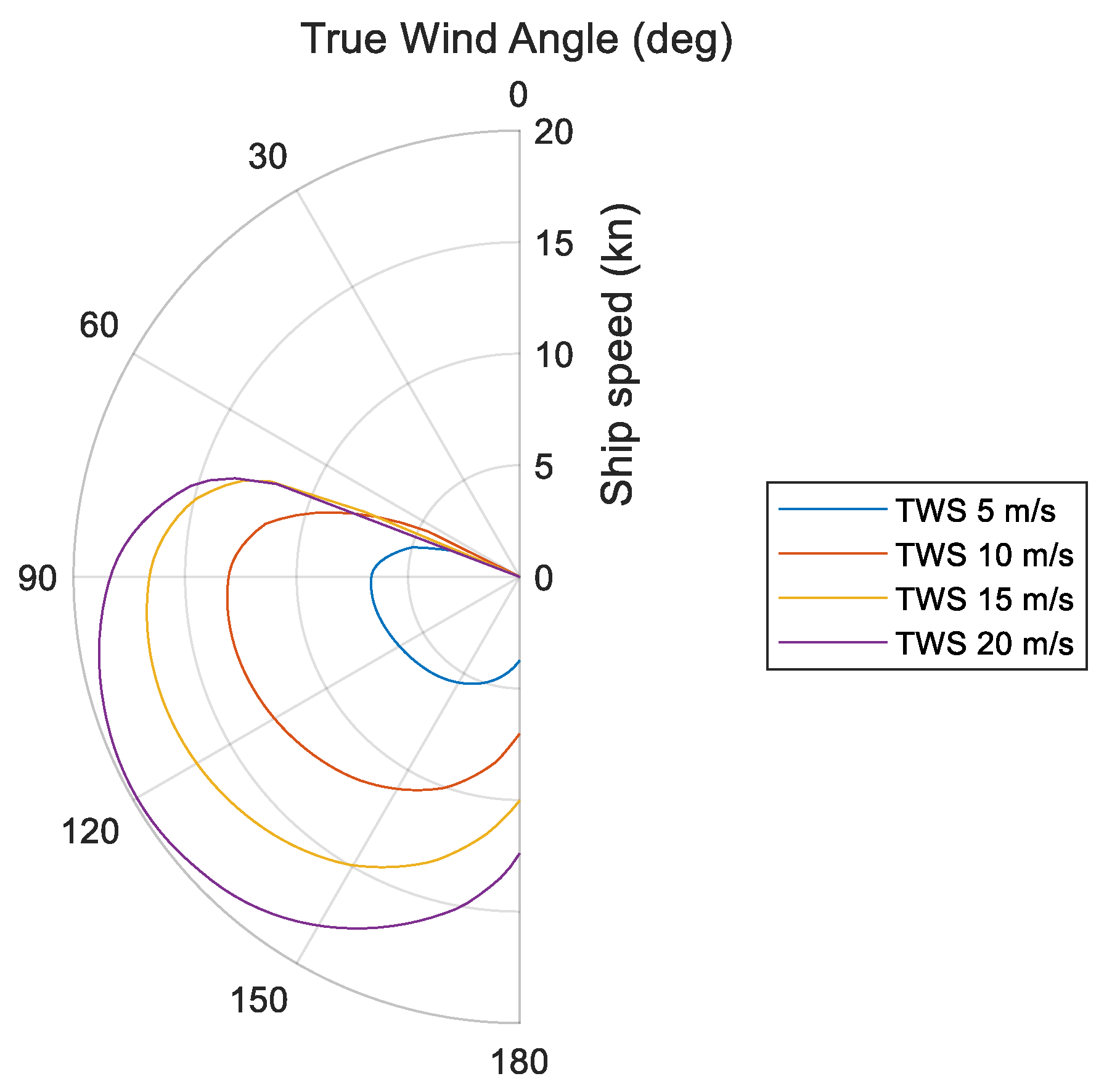
An initial evaluation was done to illustrate the ship speeds achieved with the wind propulsion system installed on board the concept ship. The results are presented in Figure 14 as a polar plot over the true wind angle and speed. The plot reflects similarities with the previously presented Figure 3 from Section 2.1.1.

A results summary is presented below and in

Table 2. Summary of simulations results for route A (Barcelona–Tunis).

Simulation	Restricted Speed	Open Speed
Average speed	5.36 knots	1.10 knots
Time	93 h	454 h
Average power consumption	729 kW	258 kW
Average power generation	149 kW	153 kW
Shore-based energy used	55702 kWh	58198 kWh

and

Table 3. Summary of simulations results for route B (Rotterdam–New York).

Simulation	Restricted Speed	Open Speed
Average speed	7.32 knots	4.29 knots
Time	448 h	765 h
Average power consumption	464 kW	305 kW
Average power generation	401 kW	395 kW
Shore-based energy used	84589 kWh	47189 kWh

.

Case (i): Route Barcelona–Tunis with limited speed

The first study case analyzes the Barcelona–Tunis route with a minimum speed of 5 knots. The voyage took (on average) 93 h, which gave an average speed of 5.3 knots. The average power consumption of the systems onboard was 729 kW, while the average power generation was 149 kW. At the end of the voyage, the energy balance showed that 55702 kWh were required in addition to the available renewable sources at sea. This is equivalent to 446 fully charged commercial marine batteries of 125 kWh each and a weight of about 713 tons, considering that each battery weighs 1.6 tons [33].

Case (ii): Route Barcelona–Tunis with open speed

The second study case analyzes the Barcelona—Tunis route when the ship speed is not restricted. The voyage took (on average) 454 h, which gave an average speed of 1.10 knots. The average power consumption of the systems onboard was 258 kW, while the average power generation was 153 kW. At the end of the voyage, the energy balance showed that 58198 kWh were required in addition to the available renewable sources at sea. This is equivalent to 474 fully charged commercial marine batteries of 125 kWh each and a weight of about 757 tons, considering that each battery weighs 1.6 tons [33].

Case (iii): Route Rotterdam–New York with limited speed

The third study case analyzes the Rotterdam–New York route for a minimum restricted speed to 5 knots. The voyage took (on average) 448 h, which gave an average speed of 7.3 knots. The average power consumption of the systems onboard was 464 kW, while the average power generation was 401 kW. At the end of the voyage, the energy balance showed that 84589 kWh were required in addition to the available renewable sources at sea. This is equivalent to 677 fully charged commercial marine batteries of 125 kWh each and a weight of about 1082 tons, considering that each battery weighs 1.6 tons [33].

Case (vi): Route Rotterdam–New York with open speed

The fourth study case analyzes the Rotterdam–New York route when the ship speed is not restricted. The voyage took (on average) 765 h, which gave an average speed of 4.3 knots. The average power consumption of the systems onboard was 305 kW, while the average power generation was 395 kW. At the end of the voyage, the energy balance showed that 47189 kWh were required in addition to the available renewable sources at sea. This is equivalent to 378 fully charged commercial marine batteries of 125 kWh each and a weight of about 604 tons, considering that each battery weighs 1.6 tons [33].

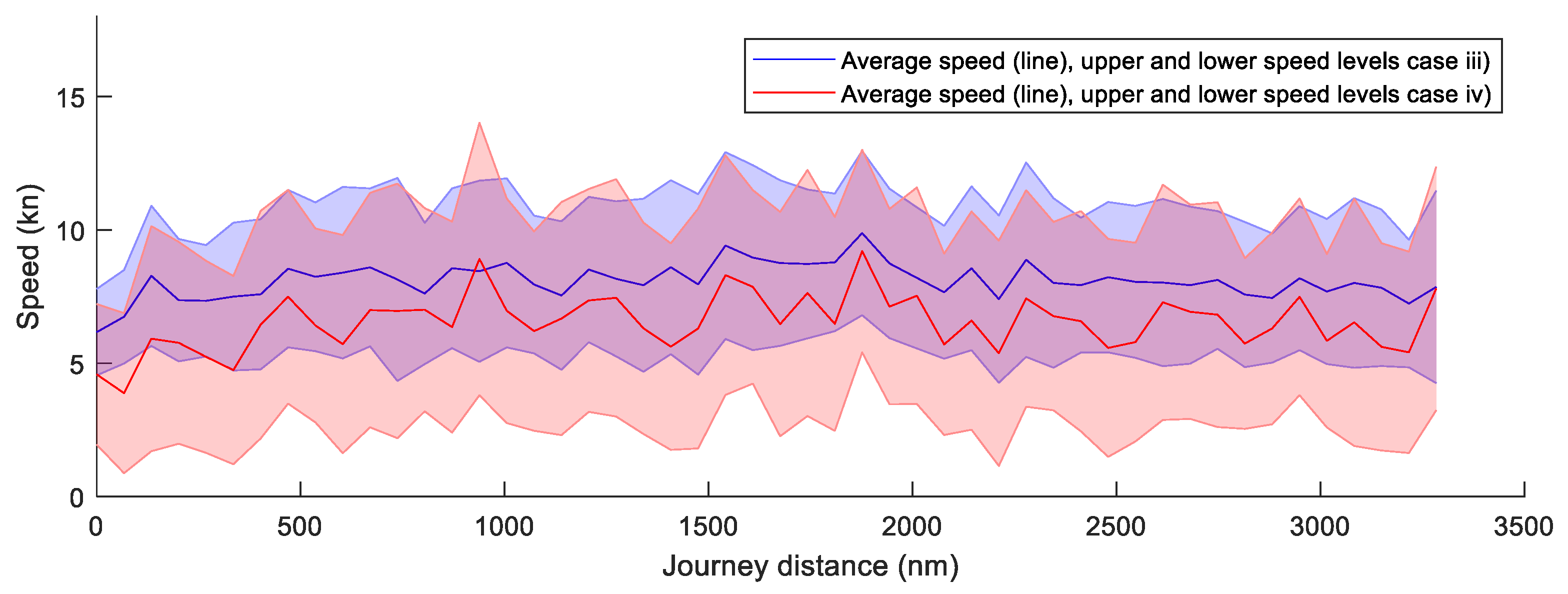
In Figure 15 and Figure 16, a comparison of the resulting ship speeds is presented for the route from Barcelona to Tunis and from Rotterdam to New York. The plots represent in blue the study cases (i) and (iii) for limited speed and in red the study cases (ii) and (vi) with open speed mode. As the result was calculated for 50 different simulations, the plot presents the average speed together with the upper and lower speed levels.

Results from route A, in Figure 15, show a considerable reduction in average ship speed (480% reduction) when moving from limited speed (case i) to open speed (case ii). The average speed for case (i) stays close to the limiting velocity; therefore, the wind propulsion is assisted with the propeller in most of the trip.

The other route B, presented in Figure 16, shows similar average and speed variation curves for both conditions (cases iii and iv). This result indicated that for both cases, the wind propulsion takes a lead role in the ship propulsion.

As a comparison between routes A and B, it is shown that from a velocity point of view, the restriction of the minimum speed of the ship is essential when considering the route A, but not as relevant in route B. In route A, the energy produced from the wind is extremely reduced in some parts of the route, and the thrust produced by the propeller eliminates those periods of low ship speed. However, route B shows that additional thrust from the propeller does not have a relevant influence to achieve the minimum speed.

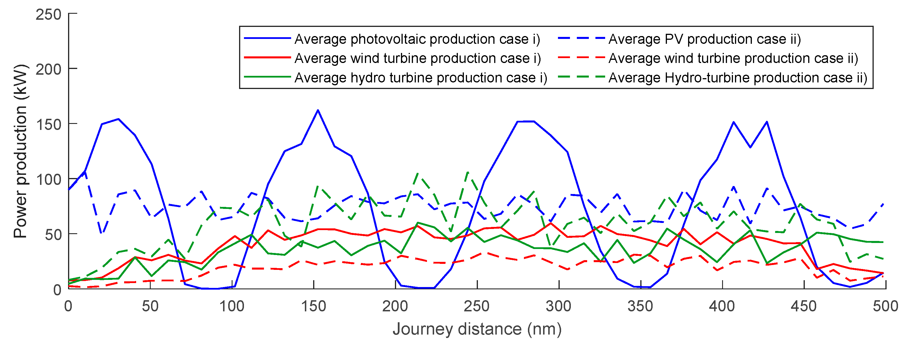
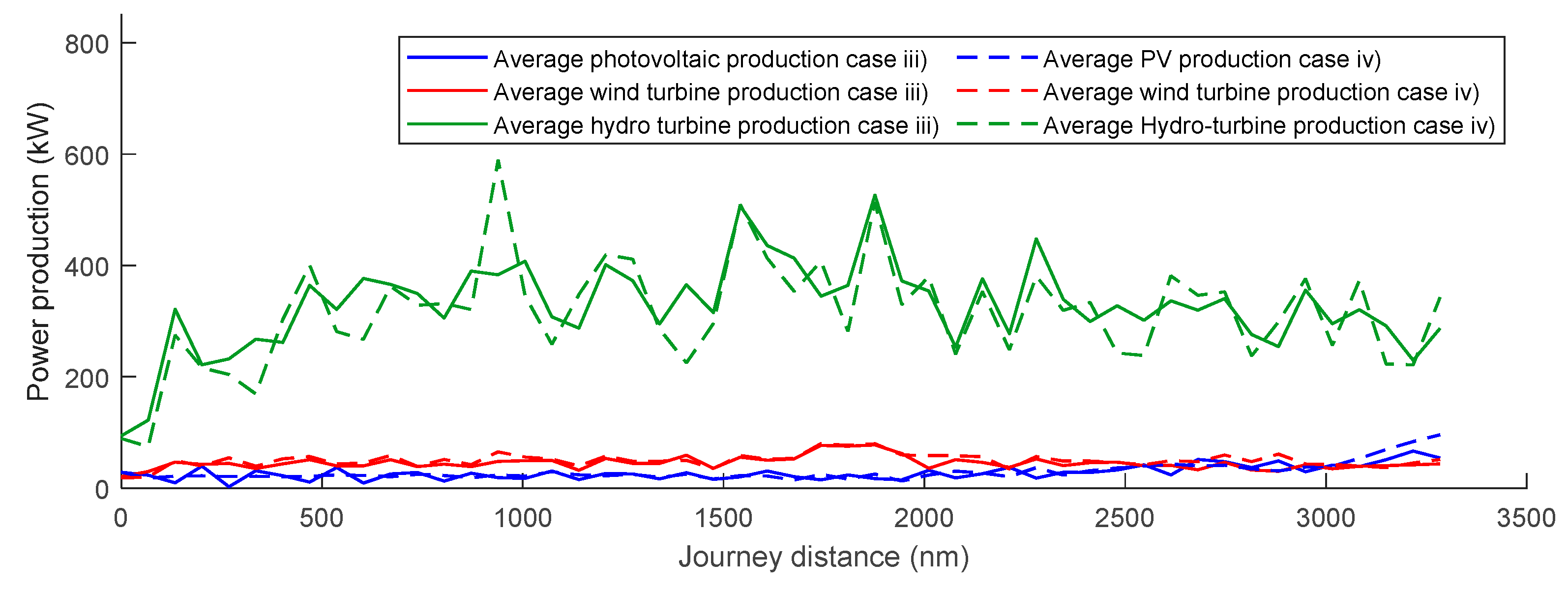
Figure 17 and Figure 18 present a comparison of the energy production for the different installed technologies. Route A is presented in Figure 17 for study cases (i) and (ii), and route B in Figure 18 for cases (iii) and (iv). The plots present the mean energy production value for solar panels, wind turbine, and hydro turbine. The plots show that for the same route, the average power production is similar despite the minimum speed restriction. Minor differences can be noticed in hydro turbine generation for route A, showing higher production levels for the open case (average case (ii) = 58.5 kW) than for limited cases (average case (i) = 36.0 kW). This is because the limited case does not sacrifice speed (increasing drag coefficient) to produce energy if the minimum speed is not reached. Comparing the routes A and B, it is noted that on route B, the energy produced by the hydro turbine becomes predominant with respect to the other technologies presented above; this is caused by stronger wind speeds and higher ship speed.

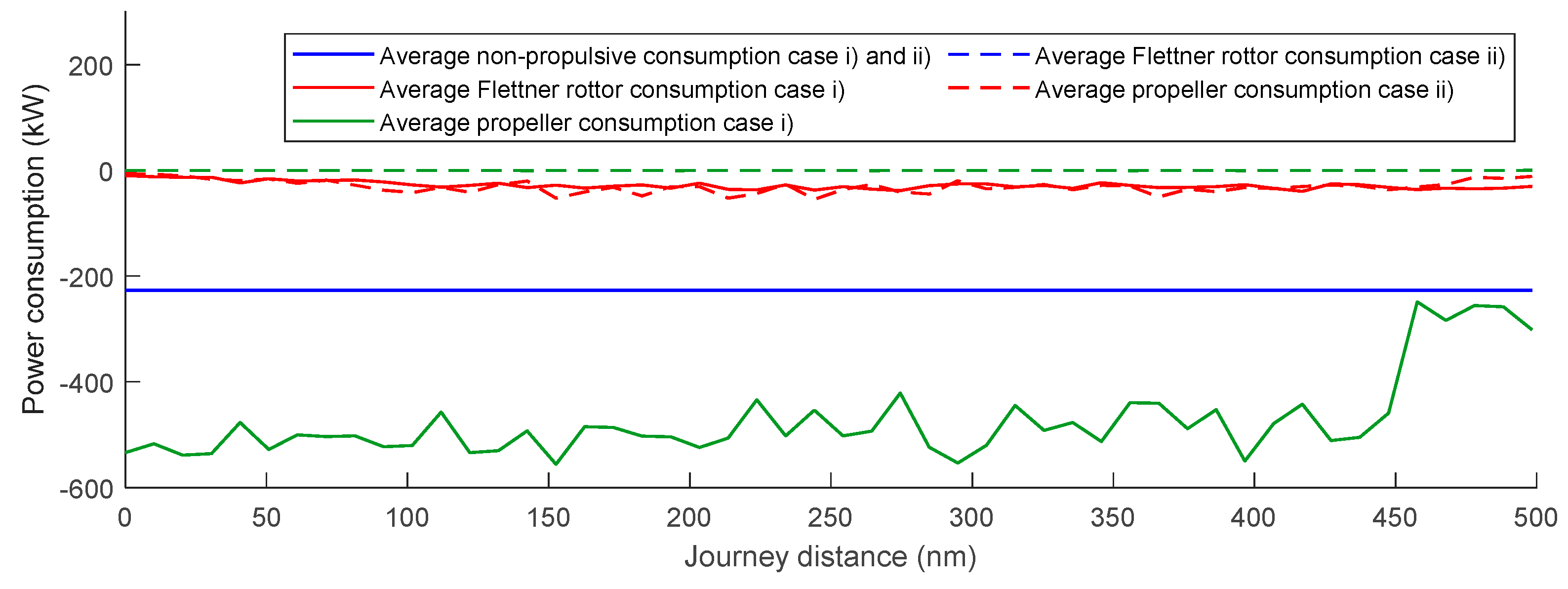
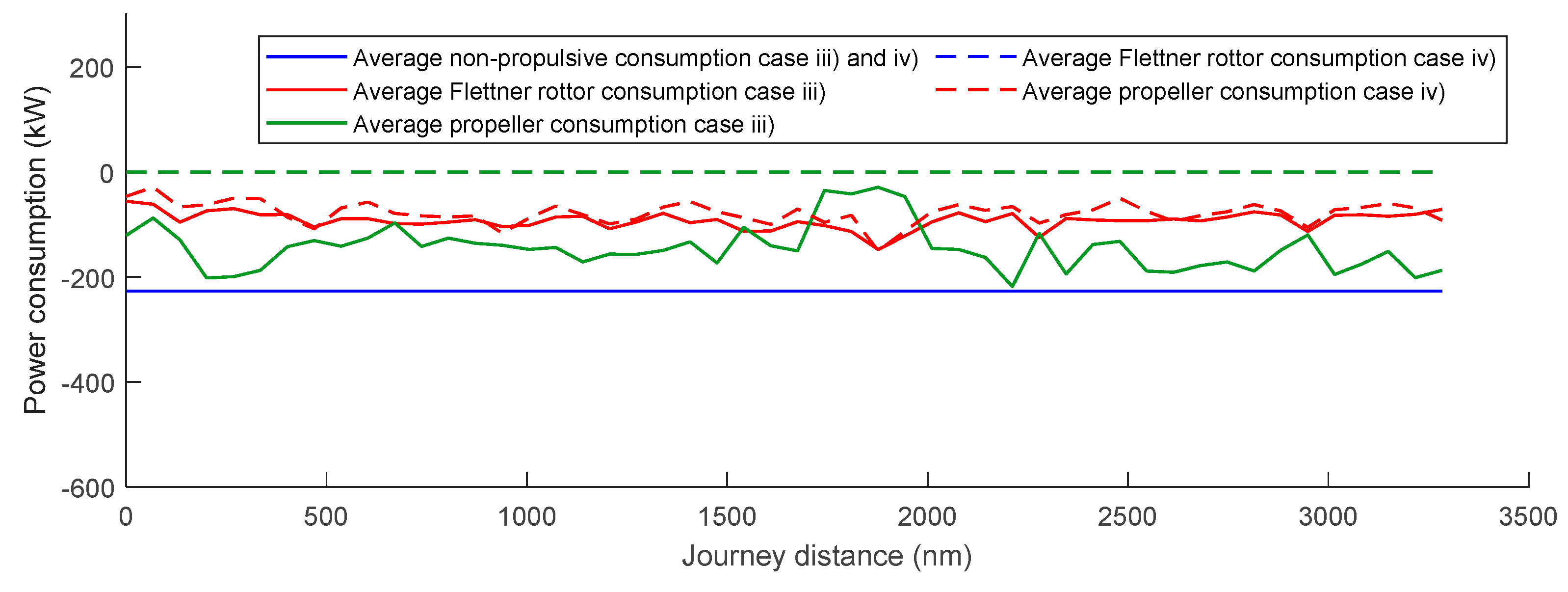
The energy consumption is presented in Figure 19 for route A and in Figure 20 for route B. The plots show the consumption of the Flettner rotors, the propeller, and the non-propulsive loads. For both routes, the propeller power demand naturally becomes zero for open speed cases (ii and iv). However, comparing the limited cases (i and iii), some differences can be noticed. Case (i) shows a mean energy demand of the propeller of 474 kW, while case (iii) has a mean value of 145 kW. These numbers highlight the influence of the propeller demand to the final ship consumption. While in case (i), propeller demand corresponds to 65% of the ship consumption, in case (iii) it corresponds to 31%. Small differences in the power demand from Flettner rotors are seen when comparing open and limited speed cases. Route B shows a slightly higher demand due to the more favorable wind conditions.

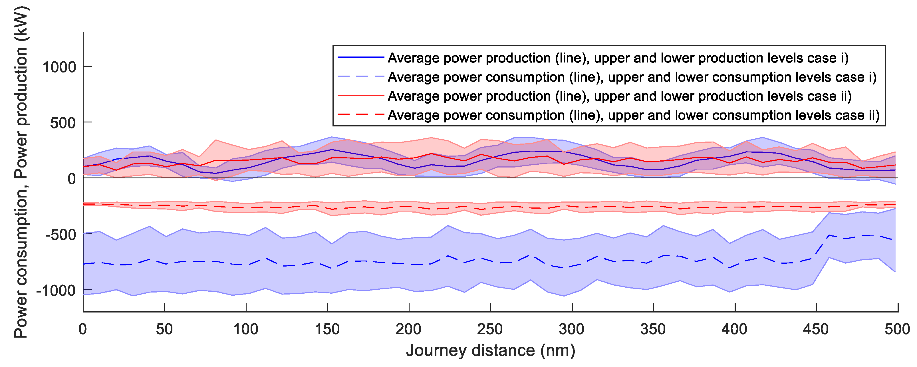
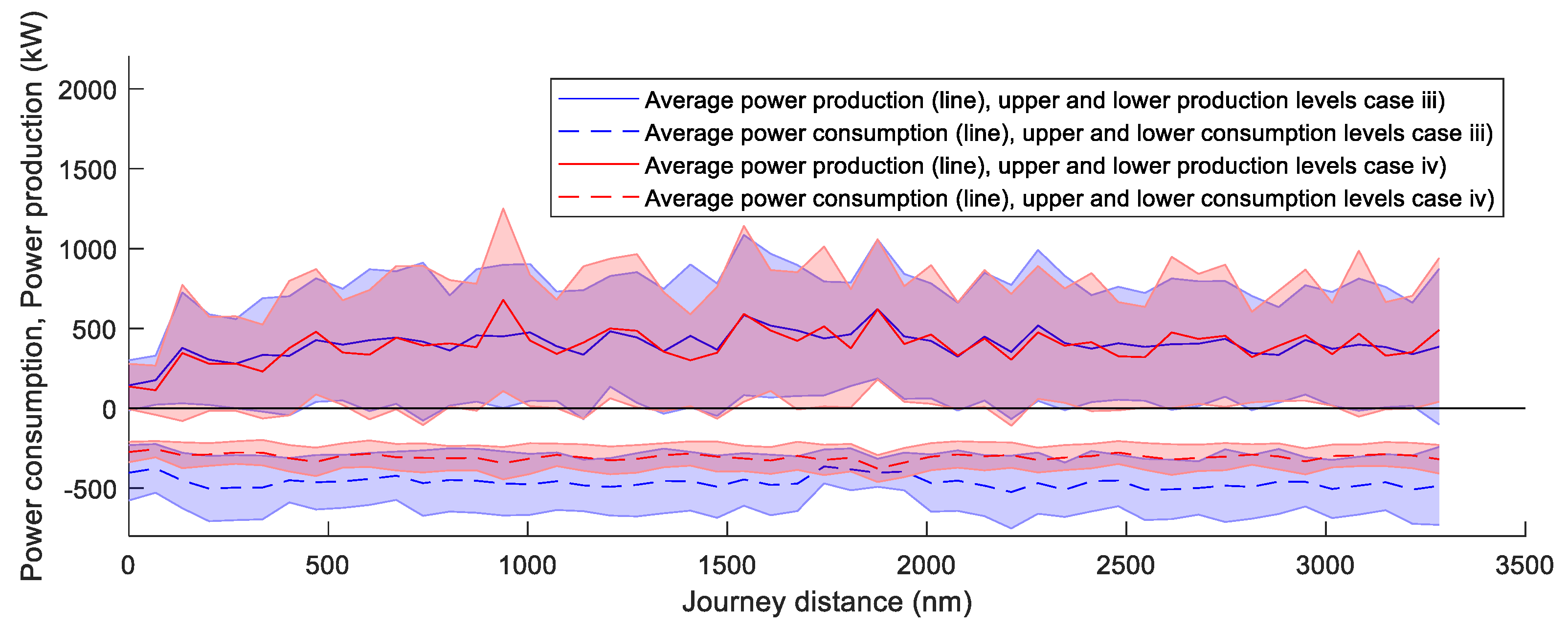
Figure 21 and Figure 22 present a comparison of the energy consumption and energy production onboard for routes A and B, respectively. The presented values are the average and upper and lower value of the consumed and produced power. The limited speed cases (i and iii) are shown in blue, and the open speed cases (ii and iv) in red. Values above zero represent power generation, values below zero power consumption.

From an energetical efficiency perspective, the results show that for route A, case (i) has an average demand of 729 kW, while the average production is 149 kW. For this case, the power required is about five times the energy produced by the renewable systems. This results in a challenging situation for the energy supply system. For the same route, case (ii), with similar average energy production (153 kW), has a smaller energy consumption of 258 kW. Even if the power balance stays in negative values, the power deficit is reduced.

The results on route B are similar for the two simulated cases (iii and iv). The average production and demand are 401 kW and 464 kW for case (iii) and 395 kW and 305 kW for case (iv), respectively.

The results show that route A is energetically less appropriate than B for the ship concept. From a power balance point of view, the restriction of the minimum speed, i.e., cases (i) and (iii), is not beneficial.

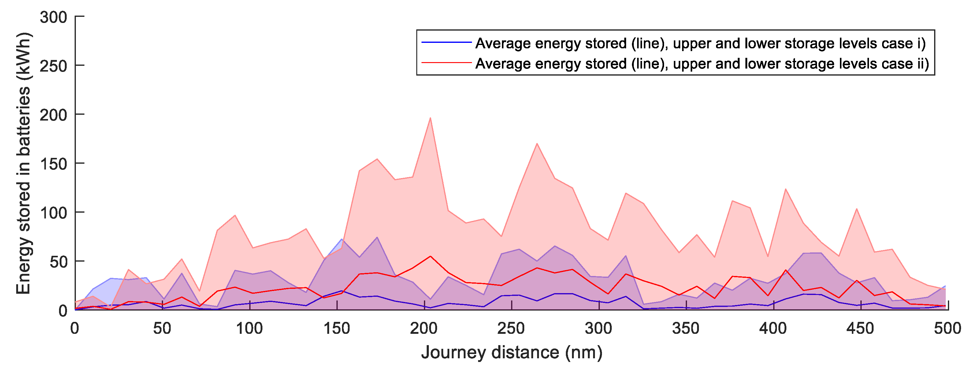
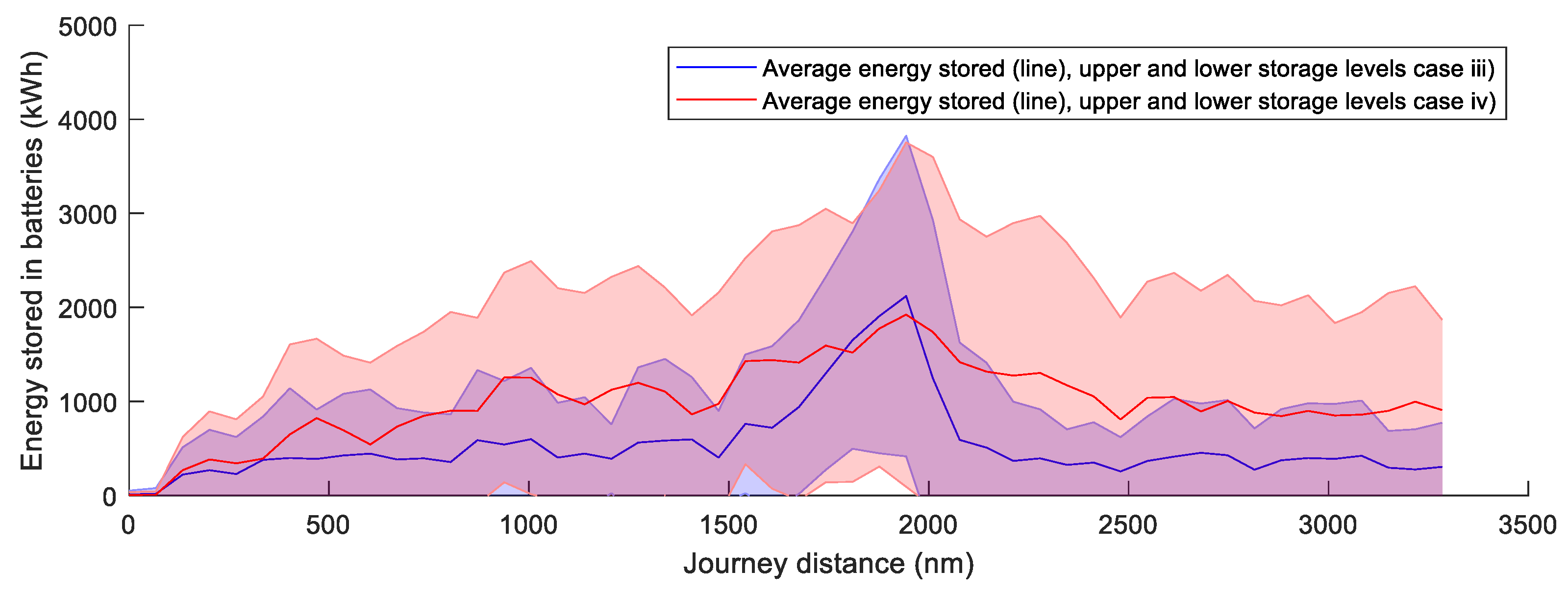
Figure 23 and Figure 24 present the average and upper and lower values for the energy accumulated in batteries. Figure 23 shows results for route A (cases i and ii) and Figure 24 for route B (cases iii and iv).

For both routes, the non-restricted speed cases (ii and iv) show better performance. Comparing the two routes, route B shows better performance with average energy stored on board of 538 kWh for case (iii) and 992 kWh for case (iv). Route A fluctuates in a range of energy stored closer to zero. Average stored energy is 7.07 kWh for case (i) and 22.4 kWh for case (ii).

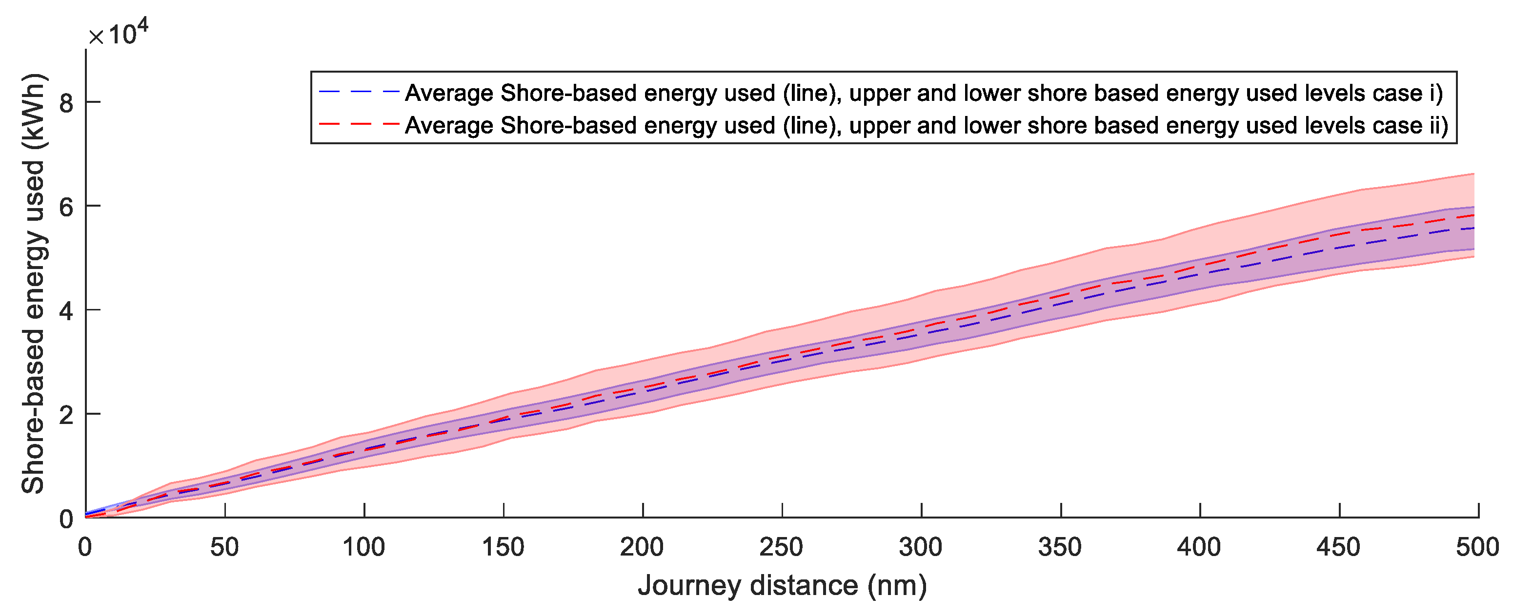
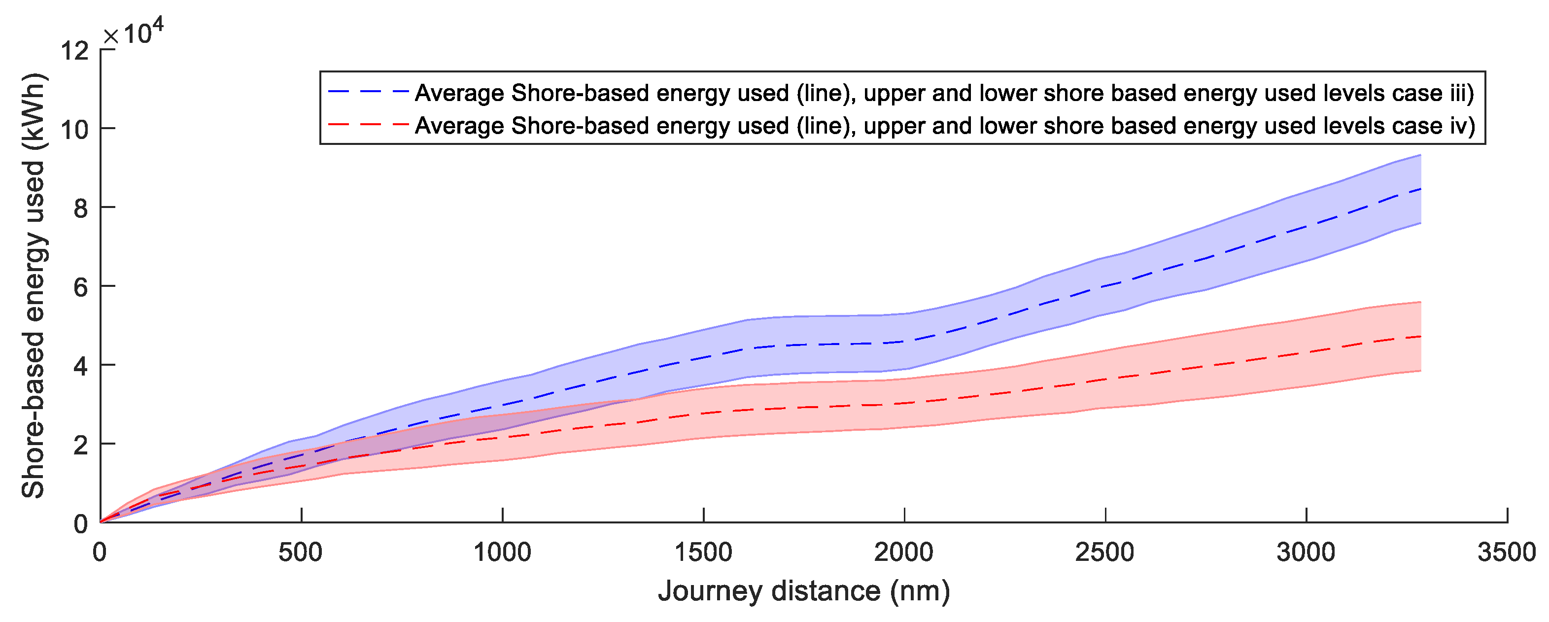
Finally, the shore-based energy consumed is shown in Figure 25 and Figure 26. Figure 25 shows results for route A (cases i and ii) and Figure 26 for route B (cases iii and iv). The figure shows the total energy required by the consumers that cannot be produced by the renewable systems beforehand.

On route A, the ship requires (on average) 55,702 kWh of shore-based energy in case (i) and 58,198 kWh in case (ii). Similar final results show that the increment in time for the route (ii) does not provide energetical benefits. On route B, the ship requires 84589 kWh in case (iii) and 47189 kWh in case (iv), on average. On this route, the energy efficiency is improved for an extended time at sea, i.e., for the case without a minimum speed limit. Considering the amount of shore-based energy used per mile, case (i) requires 112 kWh/nautical mile, case (ii) 117 kWh/nautical mile, case (iii) 25.8 kWh/nautical mile, and case (iv) 14.4 kWh/nautical mile. These results show that the efficiency and viability of sailing purely with renewable energy are considerably higher on route B.

4. Discussion and Conclusions

This study presents a novel method and model of a concept ship to evaluate the possibilities that renewable technologies can offer to the marine shipping industry. The numerical model used was developed to simulate the performance of a fossil-free operated cargo ship in realistic weather conditions. The presented methodology integrated real route conditions with the ship performance model ShipCLEAN [15,17], which simulated the ship performance using Flettner rotors together with renewable electric generators and an energy storage system to estimate the available energy. This integration made it possible to evaluate ship journey times, energy consumption, and energy production for different routes, ship types, sailing conditions, and renewable energy system configurations. Four study cases were compared, two on a Mediterranean route between Barcelona and Tunis and two on a transoceanic route between Rotterdam and New York.

• The route Barcelona—Tunis is the most challenging for a fossil-free cargo ship. The route is shorter, with favorable solar radiation but low wind speeds. The results show low ship speeds, resulting in a long time at sea (case ii) or in an increase of energy demand from the propeller to provide the additional thrust that requires much more energy than produced by renewable systems.
• Route Rotterdam—New York, has a longer distance, but the ship shows better speed performance and energy results in both study cases (iii and iv). The favorable wind conditions along most of the route provide high enough speeds to avoid the use of the propeller and to produce high energy levels with the hydro turbine. As a result, the energy balance is improved requiring less stored energy.
• In all four study cases, it has been shown that it is not possible to achieve current freight market speeds with purely renewable-powered ships. Marine shipping speeds must be readapted. Further, the sailing region and routing become important parameters for the speed selection.
• When considering the dual-mode propeller and wind turbine technology, it is essential to evaluate the balance between speed and energy production. The technology can produce high energy production, but always with a considerably high sacrifice in ship speed due to the drag force created.
• In all studied cases, energy stored in the batteries onboard before the start of the trip is required, to compensate the additional energy consumption not produced by the renewable systems (shore-based energy).

A fossil-free operated cargo ship was introduced and simulated effectively, the advantages and challenges of the renewable systems onboard were highlighted, and the multiple study cases defined those sailing conditions where a vessel with similar characteristics would provide high efficiency. The impact of the present study for future research is to demonstrate that with the existing technologies, there is the possibility to operate a fossil-free vessel. Future research from the conclusions is required to investigate how particular ship designs, renewable systems, and sailing conditions can influence the efficiency of the journey to be able to optimize a renewable power vessel for its unique operation.