3.1. ORANI-G Model
The CGE model we use in this study is based on the ORANI-G single-country, multisector comparative static model [
39]. ORANI-G has been used extensively in many policy-related decisions made in Australia and several other countries [
40,
41,
42,
43]. The ORANI model was originally developed for the Australian economy, and ORANI-G is a generic version of this model that embodies all neoclassical assumptions such as cost minimisation, utility maximisation and constant return to scale.
The database used in the model is based on the Australian 2012–2013 input–output (I/O) tables [
44] compiled by the Centre of Policy Studies, Australia. The original database has 37 industries and 37 different commodities. One of the key changes we made to the database is that we disaggregated the mining industry into two separate industries: mining_coal and mining_other. In the original database, the mining industry is an aggregation of (i) black coal, (ii) brown coal, (iii) oil, (iv) LNG, (v) gas, (vi) iron ore, (vii) bauxite, (viii) nonferrous metal, (ix) other mining and (x) mining service. We disaggregated black and brown coal from mining and added them to the new industry, mining_coal. The remaining subsectors of the mining industry are found under mining_other. This segregation was influenced by the work of Hardisty, Clark [
45], who identified that a noticeable reduction in emissions in Australia is possible just by reducing dependency on coal for energy generation. Therefore, in our study, we add a tax on coal in the form of an energy tax to incorporate this insight.
The core model consists of one government, one investor and one household.
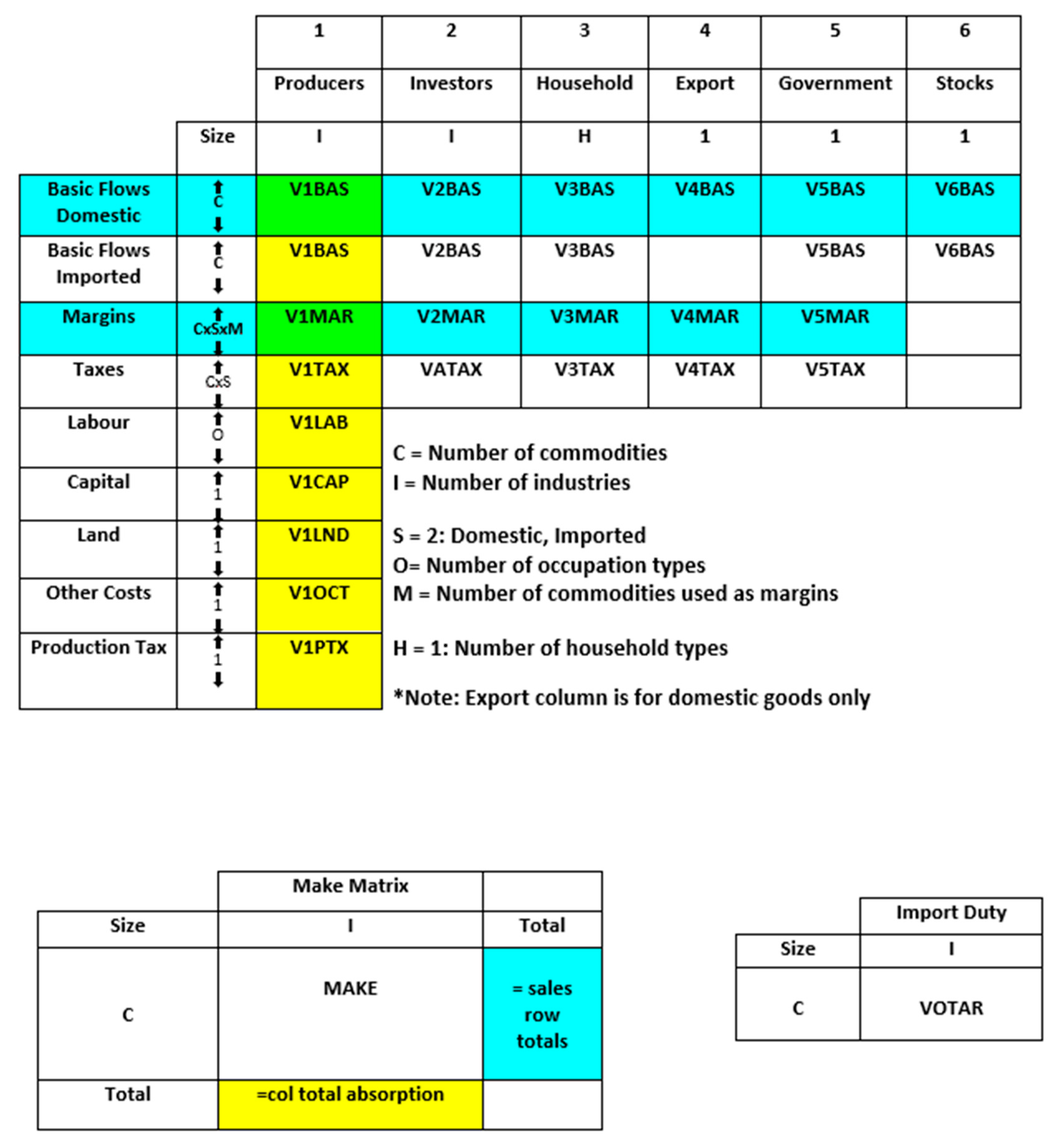
Figure A1 in
Appendix A illustrates the composition of the database. The behavioural parameters of the agents, such as Armington elasticity, labour elasticity, export demand elasticity etc. are taken from the ORANI-G model [
46].
Matrices in the first two rows (V1BAS–V6BAS) demonstrate the flow of commodities from domestic and imported sources to users. It can be translated as a flow of commodity c from domestic or imported sources to a given industry i for production, capital formation, household consumption, export, government consumption and inventories. These direct flows (domestic goods) are measured in basic prices, which are net of the margin cost and sales taxes. For imported goods, basic prices are net of margin costs and sales taxes but also include tariffs.
Matrices in the third row present the flow of domestically produced commodities that are used in margin services, namely wholesale and retail trade, utilities (electric, gas and water), financial services (banking, insurance etc.), transport and hotels.
The fourth row represents the tax paid by a user (V1TAX–V5TAX) for the usage of commodity c. V6TAX is excluded because no tax needs to be paid for inventories.
The sixth, seventh and eighth rows present the primary factor inputs, namely labour, fixed capital and agricultural land, which are used by industries to produce the commodities. In our model, labour is categorised into 97 different occupations. V1CAP and V1LND show the rental value of fixed capital and agricultural land.
Rows nine and ten exhibit the other costs and production tax, respectively. Other costs include various production costs, the cost of holding inventories and liquidity cost.
The remaining two satellite matrices present (i) the multiproduction matrix (MAKE), which presents the basic value of commodity
c produced by industry
i, and (ii) the tariff matrix, which shows the total tariff paid on imported commodity
c.
Table A1 in
Appendix A provides a summary of the I/O database used in our model. Non-negativity except taxes and inventories, zero pure profit and market clearing are the three most fundamental characteristics of the database.
We implement the productivity gain by controlling the technological change variable. In our model,
denotes the input-augmenting technical change variable, which is a vector variable with one value for each industry. The relevant equation used in the model is:
where
is the intermediate use of imported or domestic composite,
is the technological change of intermediate composite (imported or domestic) and
is the activity level or value added. All these variables are percentage change variables. If the activity level remains constant and we shock
by 5%, keeping
endogenous and
exogenous, then it would mean that
would also need to go up by 5% to keep the equation balanced. Therefore, a positive change in
implies technical regression, whereas a negative change suggests a technical advancement. We use this to calibrate the change of productivity in our model.
We followed the work of De Mooij and Bovenberg [
47], who used a 10% energy tax on energy products in a GTR context, and found it optimal for the employment dividend. We followed their approach and used an energy tax of 10% in all our simulations. In the original model, interim tax rate on any industry is represented by the variable
t, which is an endogenous variable and could, therefore, not be shocked directly. We added an exogenous shifter
with the equation of
t. The shifter
denotes uniform percentage changes in the power of tax by commodity and added shocks to energy commodities by controlling the shifter.
Lastly, in all our GTR simulations, we ensured tax revenue neutrality, meaning that all additional tax revenue generated from the energy tax was recycled back into the economy through a reduction of distortionary taxes. This revenue neutrality was ensured through a trial-and-error method. We carefully calibrated the economic shocks to coordinate a tax reform where the amount of added tax revenue and the reduction in tax revenue caused by a decline in different tax is kept equal.
3.2. Simulation Scenarios
As mentioned in the previous section, the guidelines for our GTR simulation scenarios are derived from the work on TD by Maxim [
22]. The three major findings from that metaregression study that we test in our simulations in an Australian context are (i) a reduction of payroll taxes having the highest TD potential; (ii) a reduction of other taxes, such as food tax, having a noticeable TD potential and (iii) a mixed tax revenue recycling approach using a reduction of multiple distortionary taxes being TD inducive. All these tax revenue recycling schemes are simulated coupled with the energy tax.
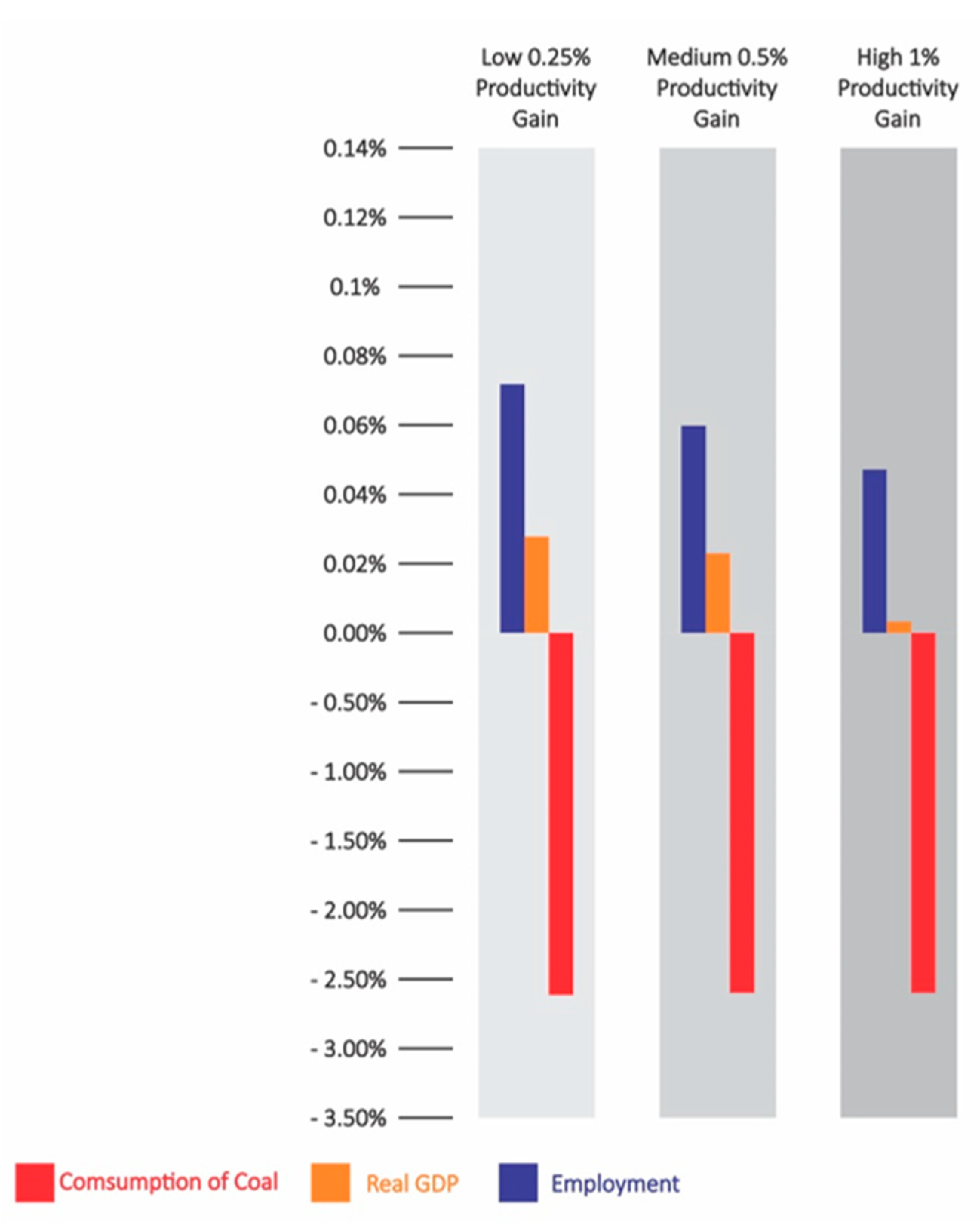
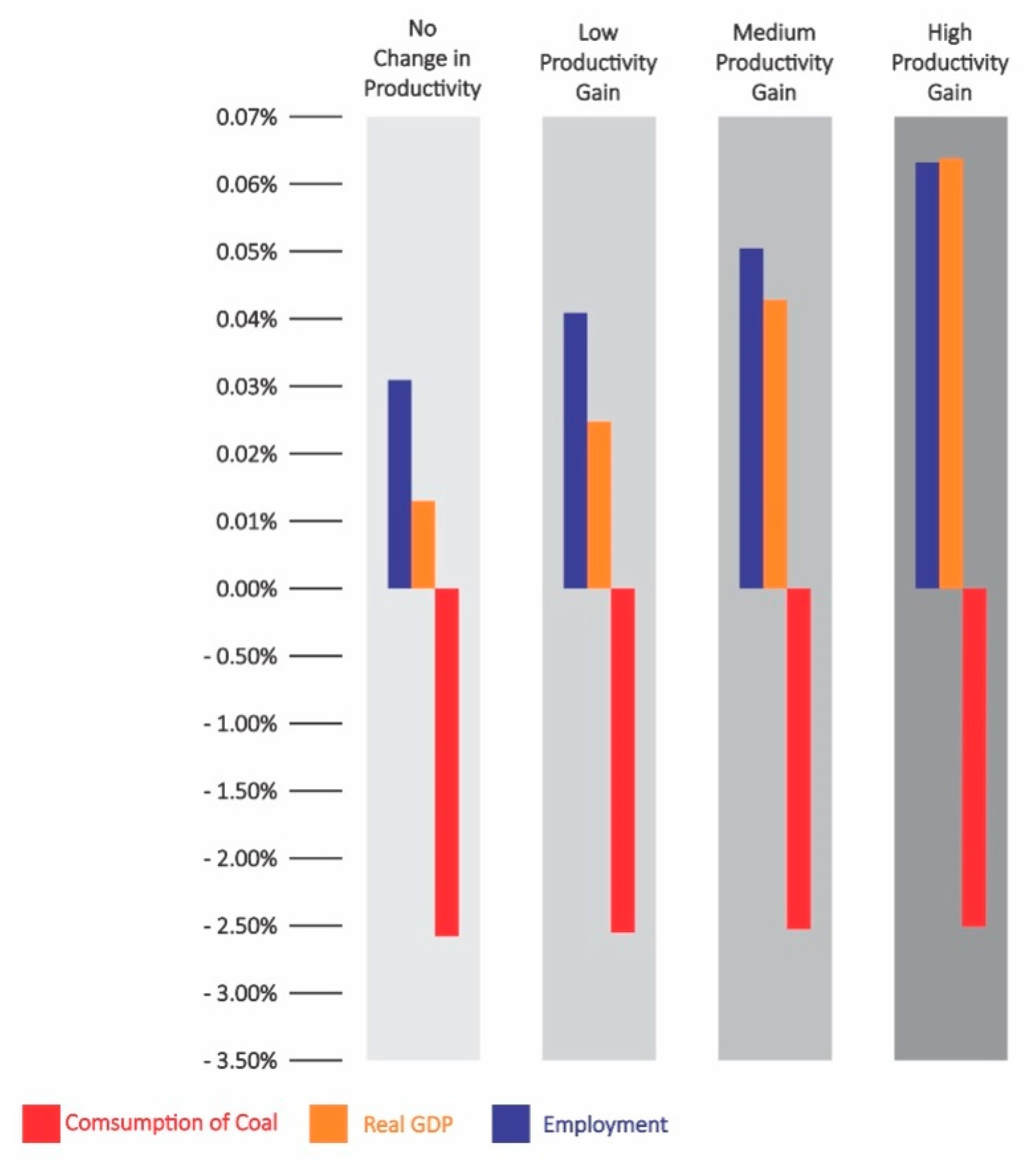
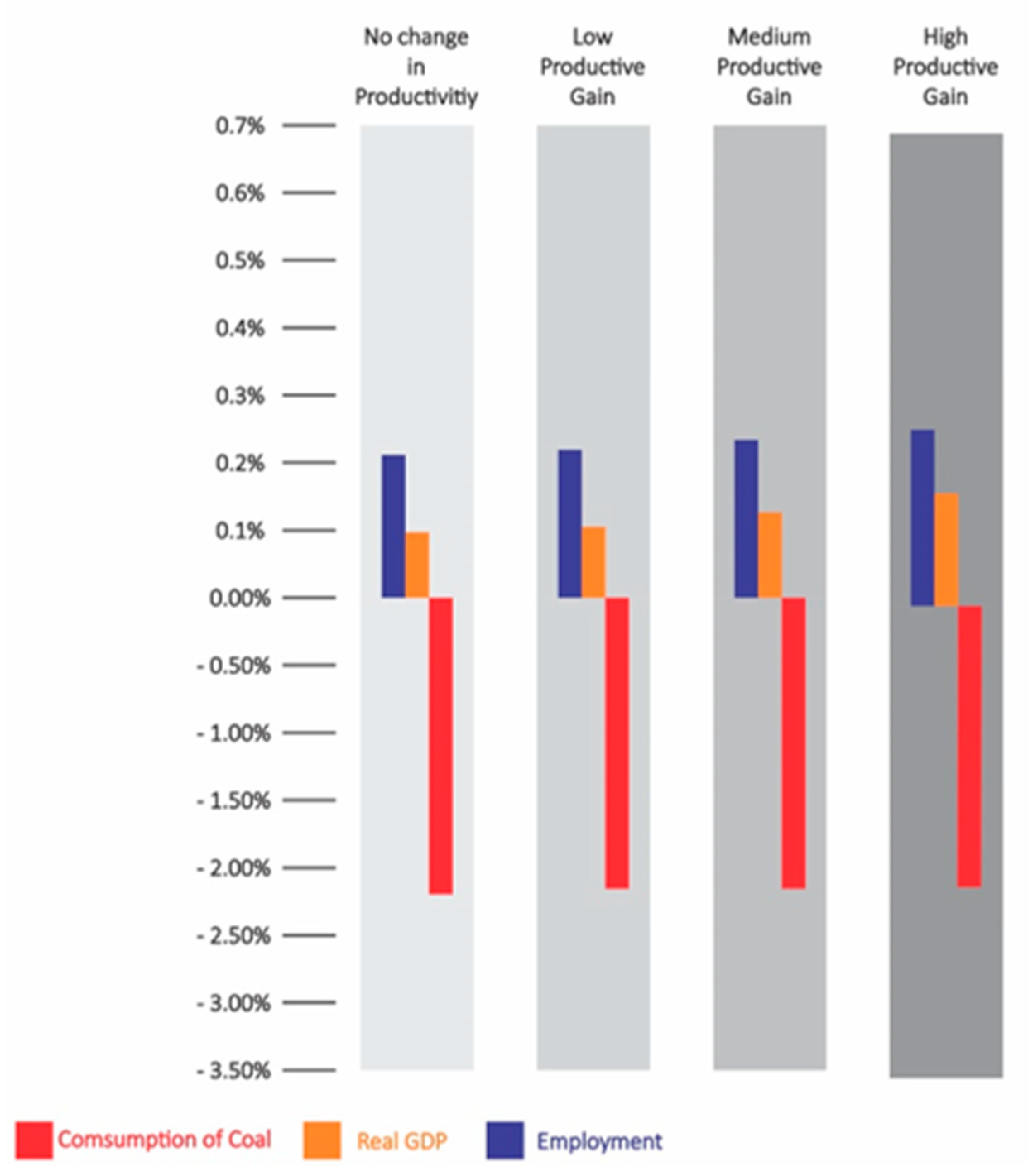
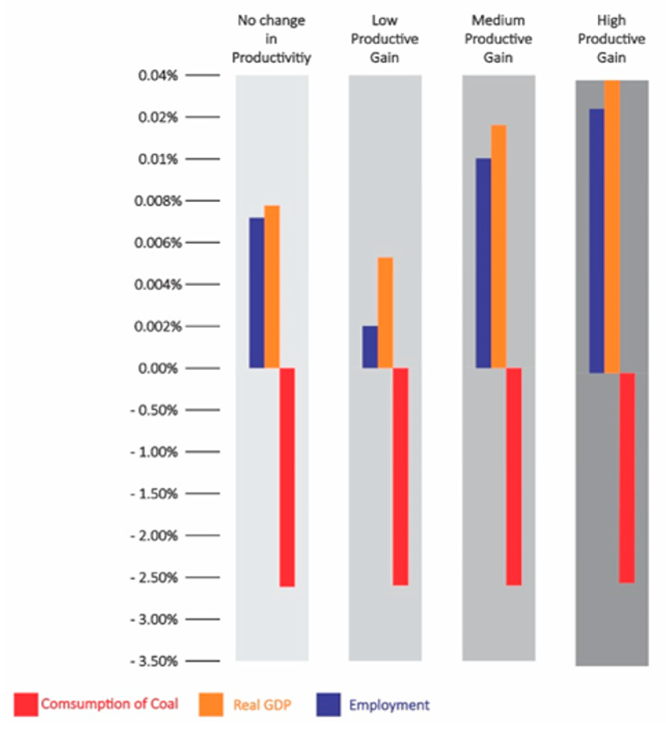
For each simulation scenario, we tested three possible productivity gain outcomes: low (0.25%), medium (0.5%) and high (1%). For a more realistic outcome, the productivity gain was limited to the agricultural industry, consisting of wheat, barley, rice, oats, other grain legumes, sugarcane, cotton, fruits and vegetables. Since productivity gain is treated as a positive externality of the primary dividend of GTR, we excluded it from the formation of GTR policy mix. We formed the basic details of the revenue-neutral GTR, such as the energy tax rate, revenue recycle scheme and reduction rate, in the absence of any productivity impact. Instead, we showed how this revenue-neutral GTR policy will perform when different levels of productivity gains are entailed by the reduction of emissions caused by the GTR.
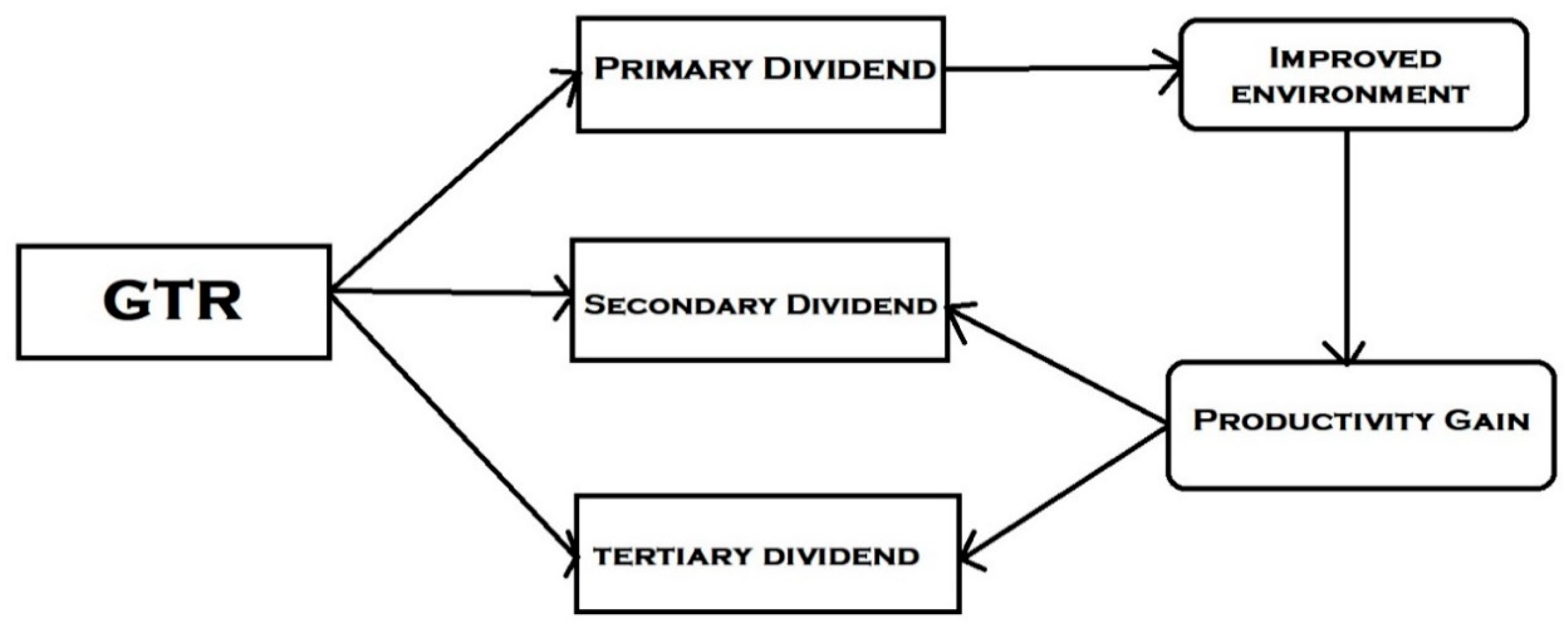
The primary dividend of GTR, which is reduction of CO
2 emissions, has already been reported time and again in the literature see [
1,
3,
4,
23,
24]. The nexus between any kind of taxation on the use of fossil fuel, leading to a lower consumption of that and, therefore, lower emissions, is quite straightforward and undisputed. The impact of such tax on the economy, however, has been the centre of enquiry. In our study, we took the primary dividend of GTR as a stylised fact and only reported the reduction of the energy product (brown and black coal) instead of incorporating any carbon counting. Our focus of measurement has been the secondary and tertiary dividends in the presence of productivity gain, and this has been reported as percentage differences from the baseline scenario. The baseline scenario measures all the factors in the absence of the GTR policies, and any difference between the baseline scenario and our simulation scenarios describes the changes driven by the GTR.
Simulation 1: In our first simulation, we tested the effect of payroll tax reduction as a form of a tax revenue recycling method in the GTR context. Reduction of payroll tax or any form of labour tax as a tax revenue recycling scheme has been strongly associated with a rise in employment in the short term when used in a GTR scenario see [
48]. The underlying reason for this nexus is the substitution between capital and labour. If some degree of substitution is possible between capital and labour, a lower payroll tax makes it cheaper for the producers to substitute capital for labour. Maxim (2020) reports that payroll tax reduction not only has the employment dividend but also has the highest TD potential. From the producers’ perspective, a reduction of payroll taxes effectively means a reduction in the wage bill that producers need to pay [
49]. In our modified version of the ORANI-G model, no form of labour tax is integrated, and therefore, we used a reduction of real wage as a proxy for a reduction of payroll tax in the first simulation. Revenue neutrality is confirmed by balancing the reduction in the total labour wage bill with the increased tax revenue driven from the energy tax.
Simulation 2: In the second simulation, we incorporated a reduction in goods and sales tax (GST) as the tax revenue recycling method. The effectiveness of food tax reduction was reported in both TD [
22] and double dividend [
3] situations. The idea was first implemented in a CGE model under the GTR context by Van Heerden, Gerlagh [
42], who demonstrated how a reduction in food tax can yield TD in the form of lower emissions, lower poverty and higher GDP. The underlying rationale behind a food tax reduction and economic dividends lies in the influence it has on households. A reduction of the tax on food, which is a necessary consumption, leads to lower household expenditure. This effectively translates to an increase in real wage from the household’s perspective. Higher real wage can lead to higher aggregate demand [
50] and can, therefore, influence both GDP and employment. Since our study is based on the Australian economy, we incorporate this method by reducing GST on some relatively essential consumptions of the household. As there is no GST on food in Australia, we lowered the GST on (i) clothing and footwear, (ii) textiles, (iii) drinks and smokes, (iv) construction, (v) transport, (vi) rubber and plastic products and (vii) chemicals.
Simulation 3: In our last simulation, we used a mixture of the revenue recycling methods of simulations two and three in a revenue-neutral GTR context to test the TD potential of a mixed-recycling approach.


