Article

Threshold or Limit? Precipitation Dependency of Austrian Landslides, an Ongoing Challenge for Hazard Mapping under Climate Change

1
Umweltbundesamt (Austrian Environment Agency), 1090 Vienna, Austria
2
Institute of Meteorology and Climatology, University of Natural Resources and Life Sciences, 1180 Vienna, Austria
3
AIT Austrian Institute of Technology, 1210 Vienna, Austria
4
Institute of Silviculture, University of Natural Resources and Life Sciences, 1180 Vienna, Austria
*
Author to whom correspondence should be addressed.
Sustainability 2020, 12(15), 6182; https://doi.org/10.3390/su12156182
Submission received: 28 May 2020 / Revised: 27 July 2020 / Accepted: 28 July 2020 / Published: 31 July 2020
(This article belongs to the Special Issue Climate Risk and Vulnerability Mapping)

Abstract

:
Climate change is set to increase landslide frequency around the globe, thus increasing the potential exposure of people and material assets to these disturbances. Landslide hazard is commonly modelled from terrain and precipitation parameters, assuming that shorter, more intense rain events require less precipitation volume to trigger a slide. Given the extent of non-catastrophic slides, an operable vulnerability mapping requires high spatial resolution. We combined heterogeneous regional slide inventories with long-term meteorological records and small-scale spatial information for hazard modelling. Slope, its (protective) interaction with forest cover, and altitude were the most influential terrain parameters. A widely used exponential threshold to estimate critical precipitation was found to incorrectly predict meteorological hazard to a substantial degree and, qualitatively, delineate the upper boundary of natural conditions rather than a critical threshold. Scaling rainfall parameters from absolute values into local probabilities (per km²) however revealed a consistent pattern across datasets, with the transition from normal to critical rain volumes and durations being gradual rather than abrupt thresholds. Scaled values could be reverted into site-specific nomograms for easy appraisal of critical rain conditions by local stakeholders. An overlay of terrain-related hazard with infrastructure yielded local vulnerability maps, which were verified with actual slide occurrence. Multiple potential for observation bias in ground-based slide reporting underlined the value of complementary earth observation data for slide mapping and early warning.

Graphical Abstract

1. Introduction

1.1. Problem Space

Landslides (henceforth “slides”), as natural disasters, threaten human health and infrastructure. Note that this article deals with the situation in Central Europe (with Austria as example), while risk and vulnerability issues probably differ elsewhere, e.g., temporary loss of agricultural production is a minor risk in this paper’s focus. Primary modes of damage are direct physical impact, undercutting of foundation, or obstruction of bottleneck line infrastructure with potentially cascading economic loss. The influence of climate change on the slide occurrence (along with other terrestrial mass movements) continues to receive much attention, and predicted consequences depend on anticipated changes in precipitation patterns [1]. An increase of rainfall extremes with climate change is both expected from theory and already observed [2,3,4,5,6,7,8,9,10], including Austria [11,12], the geographic focus of this study. In the Alps, long-term (1960–2011) seasonal shifts in slide frequency have been attributed to climate change [13].
Mapping slide risk in a changing climate faces a two-fold challenge: first, to identify appropriate precipitation triggers for slides and project their development under climate change and, second, achieve sufficient spatiotemporal resolution for meaningful delineation of exposed assets. In this work, we adopt the concept of the Intergovernmental Panel on Climate Change (IPCC ) [14] of risk as a combination of hazard, vulnerability, and exposure and consider vulnerability in its socioeconomic sense only, as opposed to biophysical vulnerability [15] (referred to here as “hazard”).
Of the three risk constituents above, social vulnerability to slide hazard is distributed relatively homogeneously across Austria, given, e.g., a nationwide Gini index around 27 [16] (on a 0 to 100 scale of increasing inequality), an observant institutional spatial planning with openly accessible hazard cadasters [17,18,19], and, last but not least, an unbureaucratic (though somewhat faceted) framework of public recompense [20,21].
Slide hazard, the second risk component, is far more variable and difficult to predict. Hazard estimation requires understanding and quantification of how meteorology interacts with a number of environmental factors to trigger a slide. Most of the environmental factors (geology, terrain, land cover) are constant compared to the velocity at which the third risk component, exposure, changes. In other words, for planning settlements or roads, geology or terrain are already well-investigated hazard constants for a given site. In fact, expert judgement of such spatial information can yield operable hazard maps at larger scales.
However, incipience and reach of landslides are typically (by frequency, not by damage caused) small-scale (tens of meters) phenomena, which require correspondingly high spatial resolution for adequate planning and protection [22].
Equally important, there remains one pivotal variable (apart from human intervention, e.g., transversal road construction) that indeed changes rapidly at a given location, namely soil water saturation. Soil water saturation modulates slide hazard via both gravitative pull and shear-strength of the affected slope. Because soil water saturation, like other small-scale drivers of slide susceptibility, is not readily observed or modelled at adequate resolution [23], considerable scientific effort has been put into predicting critical saturation levels from their main driver: precipitation. The latter is easily measured and readily available from meteorological data. Accordingly, hazard models commonly exploit the acute combination of rainfall intensity (I) and duration (D) that lead to a slide, although single studies do regard antecedent rainfall as more influential than intensity [24]. Different types of threshold functions have been suggested in numerous studies. Two comprehensive reviews [25,26] suggest the following combination of I and D:
I = a · D b
This nonlinear ID-relationship, first proposed in 1980 [27], has been adopted in these reviews as the model function to fit precipitation thresholds to data from (i) over 800+ slide events from 65 papers (mainly Europe) [25] and (ii) over 2600 observations from numerous studies worldwide [26]. Both reviews suggest Equation (1) as a generic threshold pattern. Equation (1) has two notable characteristics: (i) the exponential decline of I with D requires less precipitation volume to trigger a slide when released in a short downpour than when delivered through prolonged rainfall (implying that more frequent torrential downpours in a warming climate increase slide frequency), and (ii) it does not consider how extreme, statistically, a given rain event is for local conditions.
Apart from sufficient precipitation to trigger the slide, several environmental parameters predispose an area to slides [28]. Vegetation affects slide susceptibility both hydrologically (interception, evapotranspiration, run-off) and mechanically (roots) [29], whereby woodland has a particularly protective effect [30,31]. The protection by woodland, in turn, can suffer from climate change [32] when forest stability is affected physically (drought, fire, storm) and biologically (beneficial conditions for present and invasive pest species).
Only when hazard can be modelled at small enough spatial units—regarding the extent of slides and dispersion of infrastructure—can hazard and exposure be mapped at sufficient spatial resolution [22]. Such maps can then help reduce vulnerability by providing (i) planners with localized maps of present and future slide disposition and (ii) local authorities and individuals with threshold nomograms for rapid assessment of meteorological risk.

1.2. Rationale

As shown above, the assessment and mapping of both hazard and vulnerability requires sufficient spatial resolution. For the non-meteorological factors (geology, terrain, and forest cover), there are established GIS and modelling routines, so the most challenging part is probably the availability of sufficiently granular geodata—including reliably located slide reports.
However, the knowledge of predisposition (by non-meteorological influences) has to be complemented by a workable proxy for slide-critical soil hydrology. For mapping purposes, this proxy must be relevant and accurate at the same scale as hydrologically characteristic properties (e.g., lithology). Validating and, if necessary, advancing existing “threshold functions” of precipitation is, thus, a core requirement to map both slide hazard and vulnerability to slides.

2. Materials and Methods

2.1. Analytical Framework

2.1.1. Theoretical

We considered risk R as a product of hazard probability P and (socioeconomic) vulnerability V, the latter being the exposed asset remaining after prevention and protection measures: R = P   ( A 0 A P ) , where A 0 is the assets in reach of the hazard and A P the asset secured through measures. Probability P   has a site-specific (quasi)constant, a highly variable meteorological, and a gradually variable component (land cover, particularly forest).

2.1.2. Conceptual

We adopted a dedicated conceptual framework for vulnerability to landslides [33], which proposes total vulnerability (social and other) as a product of landslide intensity and susceptibility (of elements at risk), as shown in Figure 1.
This framework assumes total susceptibility as a sum of susceptibility components that relate to structures (susceptibility factors: type and state of maintenance), persons (income, age,) and persons in structures (abundance and strength of shielding infrastructure; population density; in our study, the stability of uphill protective forest factors as another susceptibility component). The concept also recognizes the influence of the “preparedness level” [28] and the capacity to anticipate a landslide as a susceptibility factor [34].
As explained earlier (Section 1.1), the components of social vulnerability in this framework vary comparatively little across Austria, compared to damage intensity and slide probability. The latter, i.e., how often slides strike and where, were thus the focus of our study.
In addition to prioritizing the risk (sub) components, in particular the susceptibility factors from the literature, we surveyed practitioners and stakeholders (mainly forest and natural hazard management) to gather their expert assessment of landslide risk and vulnerability in conjunction with climate change. Project outputs were further reconciled with stakeholder needs and expectations in a concluding workshop.

2.2. Data Sources

Most information (except precipitation and some slide records) was available from open or freely accessible data (Table 1).
To date, Austria shares the lack of a harmonized national slide database with many countries [28,36,37]. Consequently, we had to resort to evidence from five different sources of varying purpose, duration, administrative scope, and protocol.
The largest and longest standing of five stocks (n = 1624, ca. 50 years) originated from private damage claims. Another (n = 1533) was a public inventory with an apparent focus on road damage. Two more datasets were collected during single extreme events, thus covering large spatial variation but little temporal (and no seasonal) patterns (Figure 2).

2.3. Preprocessing

Only located and dated landslide records were considered. The accuracy of slide dates was re-checked with the originating authorities. Events with an uncertainty of more than one week were omitted (delays between occurrence, observation, and notification were common, particularly for older records).
The spatial accuracy of the largest province-wise dataset was examined by inspecting aerial photographs of the reported coordinates for a random sample of 94 recent (not older than two years) reports.
Topological data were derived from a digital elevation model using standard GIS routines except for morphology, for which we used the geomorphon package [38].
Local precipitation patterns were obtained by splitting the 50-year precipitation record of each 1 km² grid cell into segments of continuous rainfall (using breakpoints of two or more dry days in a row). Locally characteristic precipitation volumes were derived as empirical cumulative density functions for a given duration. These functions yield the extremeness (in terms of cumulative probability cp) of a given rain volume and duration at a specified square kilometer, i.e., a rain event with a cp ≥ 0.9 belongs to the top 10 percent observed at that km² during 1961–2010.
Logistic modelling of slide probability required balanced subsets of positives (observed slides) and negatives (spots where no slide was observed under identical meteorological conditions). One negative per observed slide was pinned randomly within a 300 m radius, and the terrain conditions at these spots were derived like those for the true slides.

2.4. Modelling

The following features were selected as site-specific predictors of slide probability: altitude, geology, exposition, distance to nearest forest, and slope. The following transformations were applied as suggested by the univariate distribution of features at slide sites (i.e., to approach a linear relation between predictor and slide frequency): (i) a total of 50 bedrock categories, most of which sparsely populated with slides, was transformed into a binary variable (“critical geology”) by spatiotemporal slide density; (ii) a cosine transformation of slope (angle) because slide frequency peaked at ca. 20° with symmetrical decline to shallower or steeper angles; (iii) ranking of geomorphon classes (10 classes, ranging from depression over slope to summit) by increasing slide frequency; (iv) discretization of forest distance into 10 m classes and linearization of the slightly exponential decline (sic) of slide frequency with forest distance.
Slide probability (odds ratio) was then modelled as a logistic function from the above features, including second-order interactions. Each model run used automated feature removal from the full set; models were trained with 50-fold k-validation at an 80:20 ratio of training/test observations. Prediction quality was assessed with the AUC criterion. In a complementary probabilistic approach [39], the relative importance of features for slide probability was assessed with a classification tree.
Survey responses were summarized with standard descriptive statistics, and free commentary was appraised through expert judgement, whereby responses of similar content were grouped.

2.5. Threshold Functions

Due to the comprehensiveness and significance of the meta-studies by Guzzetti and colleagues [25,26], we set out with their parametrization of the ID-function for Austria: I = 41.66 · D 0.77 (mm·h−1, h). Austria thus lies clearly in the upper intensity range (note logarithmic scale) of numerous ID-thresholds worldwide (Figure 3; note that despite similar function type, the derived critical precipitation intensity varies by an order of magnitude between studies).

2.6. Software

The following software was used: R (for modelling, particularly packages GLM for generalized linear models and the modelling frameworks caret and tidymodels), Julia (manipulation of large datasets), GRASS (processing of spatial data), QGIS (cartography), and LimeSurvey (stakeholder survey).

2.7. Uncertainty

2.7.1. Location and Date

The reliability of reported locations and dates varied, especially so for older records (when, e.g., GPS services were not readily available). Annotations in the inventories themselves or consultation with the data providers suggested that a substantial part of the records might lag the actual event by several days, particularly so before digital means became widespread in remoter areas.
The data stemming from compensation claims contained additional spatial inaccuracies: sometimes the presumable slide location was actually the claimant’s physical address, and sometimes (small) embankment movements after fresh construction works (as evident from aerials) were reported as landslides. Of a random subsample (n = 94) of this dataset, only 42% could be confirmed from aerial imagery, and another 10% were implausible (e.g., surrounded by flat, built areas).

2.7.2. Observation Bias

All data stem from individual reports, whether on private or public initiative. Reported cases, thus, are the result of cost–benefit assessment. Costs include the effort of identifying and interacting with any kind of registration service, or monitoring areas of low accessibility (altitude, terrain, infrastructure, etc.). Benefits include remuneration of damage or public savings through timely infrastructure maintenance. In fact, the fraction of false negatives in an apparently “slide-proof” area cannot be reliably ascertained without representative coverage. To illustrate, a forested hillscape may offer few slide sightings because of its robust terrain and hydrological buffers—or just because it is neither accessible nor (micro) economically vulnerable to landslides.

3. Results and Discussion

3.1. Characteristic Slide Conditions and Probable Observation Bias

The two largest inventories revealed a marked azimuthal gradient of slide frequency, as most slides were recorded on south-facing slopes. A less pronounced accumulation to the north was documented in one province-wise inventory only (Figure 4). This phenomenon has plausible physical explanations (e.g., stronger diurnal temperature gradients, exposure to precipitation-heavy Adriatic depressions in the case of the south-dominated inventory), but observation bias has to be accounted for, too. Northern slopes are more likely used for forestry or extensive grassland, so that damage will less frequently be reported or even noted. We thus opted to exclude exposition from the subsequent modelling.
The largest dataset consisted of private compensation claims to public reimbursement funds, which are processed and settled via public authority. From 1980 to 2016, most reports entered this inventory in years of local elections, followed by years when elections on a regional (provincial) level took place. Periods of no elections counted the fewest slide reports (Figure 4).
Although this suggests a reporting bias, we included all years of the particular dataset in the modelling. The bias is temporal, but hardly spatial (because elections throughout the originating province are synchronous and, thus, can be expected to affect all areas alike).
Regardless of dataset (province), slide frequency did not steadily increase with slope inclination but peaked within a range of 25° to 30° (Figure 5). Again, a contribution of observation bias cannot be excluded (steep terrain coincides with low accessibility and sparse economic assets).
As expected, slopes were the morphological feature that bore the most slides by far. About six times as many slides were observed on slopes as on spurs or hollows (Figure 5).

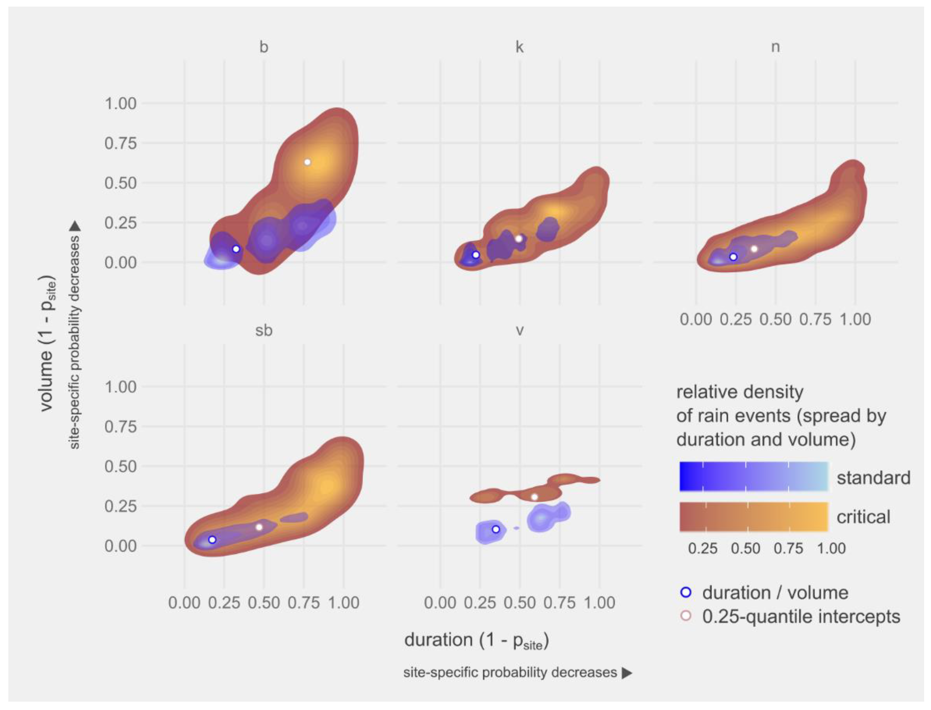
3.2. Feasibility of ID-Threshold for Local Slide Prediction

The ID-curve suggested as a country-specific threshold for Austria [25] could not be verified for our data. Even though the underlying data originated from slides within ca. 100 km distance [40], their generalization produced hazard estimates that were neither accurate nor sufficiently precise for the scales involved (main assets exposed: line infrastructure and housing). While the function did work out, in principle, for one of five provinces (although undercutting the observed volumes V by far), up to 100 percent of slides had already occurred below this threshold in the remaining four provinces. The threshold’s accuracy also changed with the duration D of the rain event (Figure 6).
Rather than forming a threshold beyond which slides would occur, the exponential ID-curve turned out to limit the range of ID-combinations—critical or not—observable in Austria (Figure 7). The ID-function was, thus, an envelope function, i.e., an upper boundary of all ID-combinations that have ever occurred in the whole province (as extracted from about 5000 50-year records), regardless of their potential to trigger a slide. Critical parameter combinations will accumulate towards the extreme of this envelope, so that retrospective inspection of only “successful” rain events (positives) will reproduce which rain conditions are possible at all rather than discern normal from critical events.
It is, thus, conceivable that the widespread form of threshold functions (Equation (1)) describes the extreme range of ID-combinations, obviously populated by disastrous events, rather than the onset of critical conditions. This is not surprising when fitting a function to a subsample of positives (=slide-effective) among all possible ID-conditions for a given area. The resulting function will describe the conditions under which a slide will most likely occur, instead of when a slide becomes likely. Limiting analysis to the upper boundary of naturally occurring rain conditions turns up somewhat counterintuitive corollaries, e.g., short downpours requiring less volume to trigger a slide. A threshold (as opposed to upper limit), in contrast, requires some kind of statistical discrimination between slide-critical and normal conditions. There are practical obstacles because negatives (uncritical combinations of precipitation parameters) are obviously not a subject of investigation and have to be reasonably assumed from climatological resources. Nevertheless, a lower boundary could be estimated from the bandwidth of critical conditions, e.g., through quantile regression.
Quantile regression in our example revealed that the intensity required for triggering a slide increased with duration. Thus, longer slide-associated rain events also have a higher average intensity and, consequentially, volume (Figure 8). A higher average intensity is a sign of steady, rich rainfalls preceding a, not necessarily extreme, ultimate event. The important role of presaturation has been pointed out by various authors (e.g., [28,41,42]), notably also for one Austrian province included here [43]. However, the considerable additional monitoring effort excludes it from many studies; antecedent rainfall factors in in less than one tenth of the 2600 observations compiled in [26].
Any attempt at deriving a threshold in absolute units (volume, duration, or a combination of both) gave poor model fits at smaller scale, and Figure 9 illustrates why. Although rain events show similar density contours, viz. slope of typical rainfall volume vs. duration, absolute values differ between drier and more humid provinces—even under otherwise identical determinants (terrain, land use, etc.).
Absolute measures of precipitation parameters (V, D, or I) thus were not suited for deriving a threshold to distinguish between standard and critical rain events. Particularly, the widespread nonlinear ID-threshold function suggested for Austria in the global comparison [25] was not only inaccurate but inconsistent, i.e., it either under- or overestimated precipitation-related slide hazard depending on province and rain duration.
We therefore standardized observations through scaling relative to a locally representative average. Such scaling has been applied by different authors using aggregates like annual precipitation (cf. [26]). Aggregates, however, only loosely approximate the actual probability (viz. extremeness) of a rain event; the probability of a downpour does not decline linearly with its deviation from average. Instead, we used the long-term empirical probability at the particular km². For instance, an extreme rainfall volume of 0.8 tops 80% of all volumes observed from 1961 to 2010 at that particular location (km²); a rain duration of 0.1 is very common (exceeded by 90% of the 50-year rainfall record for that spot). Scaling resulted in congruent patterns, regardless of dataset (province). Moreover, the standardized VD-curves turned out to be linear in the area where standard and slide-critical combinations of V and D diverge (Figure 10). This means that any threshold for critical rainfall should be found along this line, and the divide between standard and critical events can conveniently be fitted as a linear discriminant function of V and D. The critical value is then a linear combination of local probabilities of V and D. As such, it could easily be used in further models or retransformed into absolute values, e.g., as a simple precipitation hazard nomograph for handout (see below).
Describing rainfall in terms of local meteorological probability, viz. extremeness, revealed a similar ID-pattern across datasets (=provinces, precipitation regimen, etc.). Descriptors thus became instrumental once they were scaled relative to local precipitation regimen. This also suggests that, over decennia, and modulated by both large-scale influences (geology, altitude) and mesoscale intricacies (from soil hydraulics to vegetation interception and root stabilization), current landscape and its “slideable” mass reservoirs have equilibrated with precipitation to the extent where only locally extreme rain events give rise to significant mass movement.
Transforming from absolute values to local probabilities revealed the following corresponding patterns across datasets (Figure 10). Again, datasets “V” and “B” deviate from the general pattern, as these are the subsets of temporal sparse observations
  • The longer and richer (by V) a rain event, the higher the probability that it will be followed by a slide;
  • Standard and critical rains do not differ in their characteristic VD-combinations, but critical rains exceed both standard D and V;
  • An extraordinarily long-lasting rain period (high D) is more distinctive for critical rainfall than an unusually large precipitation volume;
  • Slide probability increases faster with duration than with volume of the preceding rain;
  • Standard rains hardly exceed a duration of 0.75 (local probability) and a volume of 0.25.
Figure 11 illustrates that the above linear combination of D and V has more discriminative value to discern between locally normal and critical rainfalls than either parameter alone. However, the transition is gradual and does not show a sudden variation that would qualify as a threshold. Instead, a threshold would have to be set at an arbitrary cumulative density of critical rainfalls deemed a limit for acceptable risk.
Reverting relative (by probability) V and D into absolute values based on long-term observations yielded per-km² nomographs, which give the local stakeholder an estimate of how far a particular rainfall already has developed into what is critical for the region in question (Figure 12).

3.3. Hazard Modelling and Mapping

Overall prediction quality of (logistic) regression models was poor, with an average (statistics from 50 training runs) AUC of 0.6 (on a scale from 0.5 to 1), and classification trees performed only slightly better (with an AUC of around 0.7). Slope was the single and strongest predictor for slide probability (expressed as odds ratio) and reoccurred in the most influential interaction term (slope, forest distance) and again as a morphological form. The interaction of slope and forest distance had the highest predictive value. Its positive coefficient means that slope and distance from forest combine to increase slide hazard (Table 2; only significant coefficients, p ≤ 0.05, are listed). This finding corroborates a stabilizing effect of forest on slopes.
While classification algorithms are a promising tool for hazard mapping [39] and also yielded more accurate predictions (typically around 0.8 on a 0 to 1 scale) in our example, the mechanistic regression approach is more interpretable in terms of importance and interaction of individual predictors. As such, it is also much easier to comprehend and reproduce by stakeholders than the random forest “black box”. Interestingly, altitude attained the highest parameter importance in random forest (RF) ensembles, about 1.6 times as high as slope. The different assessment from a mechanistic perspective (expert judgement/regression) or a black box probabilistic approach (RF) was also observed by [44] focusing on one of the provinces examined here. It demonstrates the different rationale between both; RF classification optimizes prediction accuracy (only) so that altitude turns out to be the most important, likely because it subsumes—for the region the RF was trained on—correlated parameters like slope, average precipitation, and geology. Regression, in turn, allows much better insight into the trend of feature dependencies including their interactions. Therefore, hazard maps were derived from the regression models.
In the present study, slope alone or in combination with forest proximity, (closely related) morphology, or altitude had the highest influence on slide susceptibility. This is illustrated by Figure 13 in which modelled hazard and observed slides concentrate in the abrupt descents from hills to valley bottoms and lakes. On a larger, province-wide scale, such accumulations were also seen along the vaults where different geologies meet (not shown). Figure 13 also shows the higher density on south-exposed terrain (compare northern and southern lake regions). Again, observation bias might play a role, as slide reports concentrate near infrastructure in the valleys and at the lakesides.
Figure 14 demonstrates how the regional model is easily converted into local overview maps (Figure 14). With standard GIS operations, slide probability can be aggregated over exposed assets and scaled with asset or reparation costs to arrive at value exposed. Such maps both reduce social vulnerability by helping locals to anticipate landslides [34] and are indispensable to assessing damage intensity, whether regarded as part of the hazard or the vulnerability [33].

4. Conclusions

In contrast to good progress in regional climate projections and modelling forest growth under climate change induced disturbances (manuscripts in preparation), the local inaccuracy of existing precipitation threshold functions turned out to be the primary obstacle for landslide risk mapping. Our results suggest that a spatially meaningful mapping requires the observance of local long-term precipitation probabilities rather than the selection of extreme cases from a regional or larger scope, which can severely mislead both short-term prevention and long-term planning endeavors. As our example demonstrates, locally representative modelling has become quite feasible with the current availability of computational and meteorological resources.
We demonstrate that the meteorological component of slide hazard has a strong local variation and provide an example of how this variation can be visualized for easy apprehension by the local population.
Our investigations turned up a number of potential and at least one actual instance of bias incurred by ground observation and the spatially, technically, and institutionally disperse array of slide documentations. These together profoundly impede a systematic examination of evidence for planning and prevention and introduce bias. The difficulties encountered underline the necessity to install and maintain a harmonized inventory of damage caused by extreme weather, which is still in its pilot stages in Austria.
The preferential observation of easily accessible and/or immediately economically vulnerable spots does not only introduce bias but is prone to overlooking potentially fatal [45] precursor flows and minor clefts in uphill zones. We therefore recommend increased exploitation of earth observation data, which is already in a semi-automated state [46], as an indispensable complement to traditional ground-based surveillance.

Author Contributions

Conceptualization, I.O., H.F., P.L., and M.J.L.; Data curation, I.O. and D.L.; Formal analysis, I.O. and P.L.; Funding acquisition, H.F. and P.L.; Investigation, A.F., H.F., N.G., D.L., A.S. and M.J.L.; Methodology, I.O., N.G., P.L. and M.J.L.; Project administration, M.J.L.; Resources, A.F., N.G. and D.L.; Software, I.O.; Supervision, H.F. and M.J.L.; Validation, A.S.; Visualization, I.O.; Writing—original draft, I.O. and M.J.L. All authors have read and agreed to the published version of the manuscript.

Funding

The results presented here are an outcome of research project GLADE, funded by the Austrian Climate & Energy Funds (Klima+Energiefonds) through the Austrian Climate Research Programme (ACRP).

Acknowledgments

Huge credit is due to our deceased colleague Martin König, who enthusiastically masterminded the conceptualization of this project to further explore the interaction between climate change vulnerability and macro economy. We are grateful to Matthews Bradley for proofreading and helpful comments on an earlier version of the manuscript. We are very grateful for the contributions of all those FOSS and open data communities to the machinery we ran our analyses and presentations with!

Conflicts of Interest

The authors declare no conflict of interest.

References

  1. Gariano, S.L.; Guzzetti, F. Landslides in a changing climate. Earth-Sci. Rev. 2016, 162, 227–252. [Google Scholar] [CrossRef] [Green Version]
  2. Allan, R.P.; Soden, B.J. Atmospheric Warming and the Amplification of Precipitation Extremes. Science 2008, 321, 1481–1484. [Google Scholar] [CrossRef] [Green Version]
  3. Crozier, M.J. Deciphering the effect of climate change on landslide activity: A review. Geomorphology 2010, 124, 260–267. [Google Scholar] [CrossRef]
  4. Min, S.-K.; Zhang, X.; Zwiers, F.W.; Hegerl, G.C. Human contribution to more-intense precipitation extremes. Nature 2011, 470, 378–381. [Google Scholar] [CrossRef]
  5. Trenberth, K.E. Changes in precipitation with climate change. Clim. Res. 2011, 47, 123–138. [Google Scholar] [CrossRef] [Green Version]
  6. Reichstein, M.; Bahn, M.; Ciais, P.; Frank, D.; Mahecha, M.D.; Seneviratne, S.I.; Zscheischler, J.; Beer, C.; Buchmann, N.; Frank, D.C.; et al. Climate extremes and the carbon cycle. Nature 2013, 500, 287–295. [Google Scholar] [CrossRef]
  7. Kendon, E.J.; Roberts, N.M.; Fowler, H.J.; Roberts, M.J.; Chan, S.C.; Senior, C.A. Heavier summer downpours with climate change revealed by weather forecast resolution model. Nat. Clim. Chang. 2014, 4, 570–576. [Google Scholar] [CrossRef] [Green Version]
  8. Paranunzio, R.; Laio, F.; Nigrelli, G.; Chiarle, M. A method to reveal climatic variables triggering slope failures at high elevation. Nat. Hazards 2015, 76, 1039–1061. [Google Scholar] [CrossRef]
  9. Westra, S.; Fowler, H.; Evans, J.; Alexander, L.; Berg, P.; Johnson, F.; Kendon, E.; Lenderink, G.; Roberts, N. Future changes to the intensity and frequency of short-duration extreme rainfall. Rev. Geophys. 2014, 52, 522–555. [Google Scholar] [CrossRef]
  10. Fischer, E.M.; Knutti, R. Anthropogenic contribution to global occurrence of heavy-precipitation and high-temperature extremes. Nat. Clim. Chang. 2015, 5, 560–564. [Google Scholar] [CrossRef]
  11. Formayer, H.; Fritz, A. Temperature dependency of hourly precipitation intensities—Surface versus cloud layer temperature: Precipitation Intensities: Surface Versus Cloud Layer Temperature. Int. J. Climatol. 2017, 37, 1–10. [Google Scholar] [CrossRef]
  12. Kellermann, P.; Bubeck, P.; Kundela, G.; Dosio, A.; Thieken, A. Frequency Analysis of Critical Meteorological Conditions in a Changing Climate—Assessing Future Implications for Railway Transportation in Austria. Climate 2016, 4, 25. [Google Scholar] [CrossRef] [Green Version]
  13. Stoffel, M.; Tiranti, D.; Huggel, C. Climate change impacts on mass movements—Case studies from the European Alps. Sci. Total Environ. 2014, 493, 1255–1266. [Google Scholar] [CrossRef]
  14. Field, C.B.; Barros, V.R.; Mastrandrea, M.D.; Mach, K.J.; Abdrabo, M.-K.; Adger, N.; Anokhin, Y.A.; Anisimov, O.A.; Arent, D.J.; Barnett, J.; et al. Summary for policymakers. In Climate Change 2014: Impacts, Adaptation, and Vulnerability. Part a: Global and Sectoral Aspects. Contribution of Working Group II to the Fifth Assessment Report of the Intergovernmental Panel on Climate Change; Cambridge University Press: Cambridge, UK, 2014; pp. 1–32. [Google Scholar]
  15. Brooks, N. Vulnerability, risk and adaptation: A conceptual framework. Tyndall Cent. Clim. Chang. Res. Work. Pap. 2003, 38, 1–16. [Google Scholar]
  16. Luptáčik, M.; Nežinský, E. Measuring income inequalities beyond the Gini coefficient. Cent. Eur. J. Oper. Res. 2020, 28, 561–578. [Google Scholar] [CrossRef] [Green Version]
  17. Hlatky, T. HORA—An Austrian platform for natural hazards. In Proceedings of the EGU General Assembly Conference Abstracts. 2009, p. 8453. Available online: https://ui.adsabs.harvard.edu/abs/2009EGUGA..11.8453H/abstract (accessed on 15 June 2020).
  18. Rudolf-Miklau, F. Principles of hazard assessment and mapping. Wildbach Lawinenverbau Z. Wildbach Lawinen Eros. Steinschlagschutz 2011, 166, 20–29. [Google Scholar]
  19. Wöhrer-Alge, M. Landslide Management in Austria with Particular Attention to Hazard Mapping and Land Use Planning. In Landslide Science and Practice; Margottini, C., Canuti, P., Sassa, K., Eds.; Springer: Berlin/Heidelberg, Germany, 2013; pp. 231–237. ISBN 978-3-642-31312-7. [Google Scholar]
  20. Holub, M.; Fuchs, S. Mitigating mountain hazards in Austria—Legislation, risk transfer, and awareness building. Nat. Hazards Earth Syst. Sci. 2009, 9, 523–537. [Google Scholar] [CrossRef] [Green Version]
  21. Schinko, T.; Mechler, R.; Leitner, M.; Hochrainer-Stigler, S. Iterative Climate Risk Management as Early Adaptation in Austria–Policy Case Study: Public Adaptation at the Federal & Provincial Level; PACINAS Working Paper# 03. 2017. Available online: http://anpassung.ccca.at/pacinas/wp-content/uploads/sites/3/2017/06/PACINAS_Working_Paper-03_final.pdf (accessed on 15 June 2020).
  22. Stark, C.P.; Hovius, N. The characterization of landslide size distributions. Geophys. Res. Lett. 2001, 28, 1091–1094. [Google Scholar] [CrossRef]
  23. van Westen, C.J.; Castellanos, E.; Kuriakose, S.L. Spatial data for landslide susceptibility, hazard, and vulnerability assessment: An overview. Eng. Geol. 2008, 102, 112–131. [Google Scholar] [CrossRef]
  24. Field, C.B.; Barros, V.; Stocker, T.F.; Dahe, Q. Managing the Risks of Extreme Events and Disasters to Advance Climate Change Adaption: Special Report of the Intergovernmental Panel on Climate Change; Intergovernmental Panel on Climate Change, Field, C.B., Eds.; Cambridge University Press: New York, NY, USA, 2012; ISBN 978-1-107-02506-6. [Google Scholar]
  25. Guzzetti, F.; Peruccacci, S.; Rossi, M.; Stark, C.P. Rainfall thresholds for the initiation of landslides in central and southern Europe. Meteorol. Atmos. Phys. 2007, 98, 239–267. [Google Scholar] [CrossRef]
  26. Guzzetti, F.; Peruccacci, S.; Rossi, M.; Stark, C.P. The rainfall intensity–duration control of shallow landslides and debris flows: An update. Landslides 2008, 5, 3–17. [Google Scholar] [CrossRef]
  27. Caine, N. The Rainfall Intensity—Duration Control of Shallow Landslides and Debris Flows. Geogr. Ann. Ser. Phys. Geogr. 1980, 62, 23–27. [Google Scholar] [CrossRef]
  28. Nadim, F. Landslide Hazard and Risk Assessment; Words into Action Guidelines: National Disaster Risk Assessment. UNISDR. 2017, p. 10. Available online: https://www.preventionweb.net/files/52828_03landslidehazardandriskassessment.pdf (accessed on 15 June 2020).
  29. Preti, F. Forest protection and protection forest: Tree root degradation over hydrological shallow landslides triggering. Ecol. Eng. 2013, 61, 633–645. [Google Scholar] [CrossRef]
  30. Dolidon, N.; Hofer, T.; Jansky, L.; Sidle, R. ‘Watershed and Forest Management for Landslide Risk Reduction’, in Landslides—Disaster Risk Reduction; Sassa, K., Canuti, P., Eds.; Springer: Berlin/Heidelberg, Germany, 2009; pp. 633–649. [Google Scholar]
  31. Rickli, C.; Bebi, P.; Graf, F.; Moos, C. Shallow Landslides: Retrospective Analysis of the Protective Effects of Forest and Conclusions for Prediction. In Recent Advances in Geotechnical Research; Wu, W., Ed.; Springer Series in Geomechanics and Geoengineering; Springer International Publishing: Cham, Switzerland, 2019; pp. 175–185. ISBN 978-3-319-89670-0. [Google Scholar]
  32. Dale, V.H.; Joyce, L.A.; Mcnulty, S.; Neilson, R.P.; Ayres, M.P.; Flannigan, M.D.; Hanson, P.J.; Irland, L.C.; Lugo, A.E.; Peterson, C.J.; et al. Climate Change and Forest Disturbances. BioScience 2001, 51, 723. [Google Scholar] [CrossRef] [Green Version]
  33. Uzielli, M.; Nadim, F.; Lacasse, S.; Kaynia, A.M. A conceptual framework for quantitative estimation of physical vulnerability to landslides. Eng. Geol. 2008, 102, 251–256. [Google Scholar] [CrossRef]
  34. Amatruda, G.; Bonnard, C.; Castelli, M.; Forlati, F.; Giacomelli, L.; Morelli, M.; Paro, L.; Piana, F.; Pirulli, M.; Polino, R.; et al. A key approach: The IMIRILAND project method. In Identification and Mitigation of Large Landslide Risks in Europe; CRC Press: Boca Raton, FL, USA, 2004; pp. 31–62. [Google Scholar]
  35. Hiebl, J.; Frei, C. Daily precipitation grids for Austria since 1961—Development and evaluation of a spatial dataset for hydroclimatic monitoring and modelling. Theor. Appl. Climatol. 2018, 132, 327–345. [Google Scholar] [CrossRef]
  36. Schweigl, J.; Hervás, J. Landslide Mapping in Austria. JRC Sci. Tech. Rep. 2009. Available online: https://core.ac.uk/download/pdf/38617857.pdf (accessed on 15 June 2020).
  37. Petschko, H.; Brenning, A.; Bell, R.; Goetz, J.; Glade, T. Assessing the quality of landslide susceptibility maps —Case study Lower Austria. Nat. Hazards Earth Syst. Sci. 2014, 14, 95–118. [Google Scholar] [CrossRef] [Green Version]
  38. Jasiewicz, J.; Stepinski, T.F. Geomorphons—A pattern recognition approach to classification and mapping of landforms. Geomorphology 2013, 182, 147–156. [Google Scholar] [CrossRef]
  39. Chen, W.; Xie, X.; Wang, J.; Pradhan, B.; Hong, H.; Bui, D.T.; Duan, Z.; Ma, J. A comparative study of logistic model tree, random forest, and classification and regression tree models for spatial prediction of landslide susceptibility. CATENA 2017, 151, 147–160. [Google Scholar] [CrossRef] [Green Version]
  40. Moser, M.; Hohensinn, F. Geotechnical aspects of soil slips in Alpine regions. Eng. Geol. 1983, 19, 185–211. [Google Scholar] [CrossRef]
  41. Crosta, G. Regionalization of rainfall thresholds: An aid to landslide hazard evaluation. Environ. Geol. 1998, 35, 131–145. [Google Scholar] [CrossRef]
  42. Ponziani, F.; Berni, N.; Stelluti, M.; Zauri, R.; Pandolfo, C.; Brocca, L.; Moramarco, T.; Salciarini, D.; Tamagnini, C. Landwarn: An Operative Early Warning System for Landslides Forecasting Based on Rainfall Thresholds and Soil Moisture. In Landslide Science and Practice; Margottini, C., Canuti, P., Sassa, K., Eds.; Springer: Berlin/Heidelberg, Germany, 2013; pp. 627–634. ISBN 978-3-642-31444-5. [Google Scholar]
  43. Poltnig, W.; Baek, R.; Berg, W.; KERŠMANC, T. Runout-modelling of shallow landslides in Carinthia (Austria). Austrian J. Earth Sci. 2016, 109. [Google Scholar] [CrossRef]
  44. Nachappa, T.G.; Kienberger, S.; Meena, S.R.; Ho, D. Comparison and validation of per-pixel and object-based approaches for landslide susceptibility mapping. Geomat. Nat. Hazards Risk 2020, 11, 572–600. [Google Scholar]
  45. Lacroix, P.; Bièvre, G.; Pathier, E.; Kniess, U.; Jongmans, D. Use of Sentinel-2 images for the detection of precursory motions before landslide failures. Remote Sens. Environ. 2018. [Google Scholar] [CrossRef]
  46. Hölbling, D.; Eisank, C.; Albrecht, F.; Vecchiotti, F.; Friedl, B.; Weinke, E.; Kociu, A. Comparing Manual and Semi-Automated Landslide Mapping Based on Optical Satellite Images from Different Sensors. Geosciences 2017, 7, 37. [Google Scholar] [CrossRef] [Green Version]
Figure 1. Risk components of (a) generic concept and (b) vulnerability concept by [33]. Note that damage intensity as a subcomponent shifts between both concepts. s1…sn: susceptibility components. Probability is highlighted, as it turned out to be the most variable and least defined component in the framework.
Sustainability 12 06182 g001
Figure 2. Temporal distribution of slide inventories from five Austrian provinces. Note the narrow observation windows for inventories B and V: These are compilations of single large range catastrophic rain events.
Sustainability 12 06182 g002
Figure 3. A regional ID-threshold for Austria (black line) compared to 42 other local to global thresholds. Modified from illustration in [25].
Sustainability 12 06182 g003
Figure 4. (a) Most slides occurred on south-facing slopes; (b) annual slide reports reach their highest counts in years of local elections (1980–2016; values: slide count per year and annual precipitation volume).
Sustainability 12 06182 g004
Figure 5. (a) The relative frequency of slides peaked between 15° and 30°, depending on province; (b) among morphological features, slopes were by far most prone to slides.
Sustainability 12 06182 g005
Figure 6. A precipitation threshold in absolute units fails to predict slide hazard (dots: rain events cumulating in a slide, shaded: fraction of triggering events observed below the country-specific threshold suggested in [26]).
Sustainability 12 06182 g006
Figure 7. An exponential decline of intensity with duration draws an envelope rather than a threshold for slide-critical combinations of rain intensity and duration (red curve: a countrywide threshold function in a common exponential form; black line: a linear function indicating the first quartile of slide-critical intensity at a given duration). See Figure 2 for the deviating pattern observed in provinces “B” and “V”.
Sustainability 12 06182 g007
Figure 8. A logarithmic increase of V with D (as required under the assumption of an exponential ID-threshold) forms an envelope (red curve) rather than a threshold (black line) for slide-critical combinations. Moreover, a linear threshold is also consistent for sparse observation sets (“B” and “V”, compare Figure 7).
Sustainability 12 06182 g008
Figure 9. Probability density of rain periods, depending on duration and volume (“standard”: 11,000–60,000 rain events per province from 1961 to 2010; “trigger”: 700–1600 rain events preceding a slide).
Sustainability 12 06182 g009
Figure 10. Characteristic VD-combinations for standard (50-year records) and potentially slide-critical (rainfall preceded a slide) rainfalls (single events, n = 3000–60,000, replaced by density clouds; brighter areas indicate that more rainfalls were observed at the VD-combination; dots: intersections of 25th percentiles of scaled variables).
Sustainability 12 06182 g010
Figure 11. Local probabilities of (a) volume or (b) duration have less discriminative value than (c) a linear combination of both dimensions, but the transition between normal and critical VD-combinations is gradual rather than a pronounced threshold.
Sustainability 12 06182 g011
Figure 12. Example of a local (per km²) rain hazard chart for laymen; darker regions indicate that the rainfall has proceeded further towards critical VD-combinations (blues: values of the discriminant function scaled from 0 to 1, most to least typical for this spot, and classed as intervals of 0.2).
Sustainability 12 06182 g012
Figure 13. Overlay of modelled landslide hazard (saturation of red increases with odds of a slide) and actual slide observations. Slides occurred almost exclusively in the “red zone”, which in turn is primarily defined by steepness of terrain (base map: basemap.at).
Sustainability 12 06182 g013
Figure 14. Masking the hazard map outside an appropriate buffer allows a rapid insight into vulnerable road sections. Red: modelled risk (risk increasing with deeper shade). Stars: actual slides (base map: basemap.at).
Sustainability 12 06182 g014
Table 1. Data used.
Table 1. Data used.
FeatureTypeRes 1Source
1slidespoint province administrations 2
2geologypolygon GBA 3 via Geoland.at 4
3elevationraster10Geoland.at
4slope, exposition (azimuth)raster10derived from (1) with a 70 × 70 moving window
5morphologyraster10derived from 1
6forest coverraster30BFW 5
7infrastructurevector OpenStreetMap
8precipitationraster1000, 1ZAMG 6 [35]
9aerials of slide sitesrastervaryingBing
10expert risk and trend assessments own data (survey)
1 resolution in meters, days; 2 scope and purpose varying per province; 3 Geologische Bundesanstalt (Austrian Federal Geological Agency); 4 Austrian open data hub; 5 Bundesforschungszentrum für Wald (Austrian Federal Forest Research Center); 6 Zentralanstalt für Meteorologie und Geodynamic (Central Agency for Meteorology and Geodynamics).
Table 2. Significant 1 model coefficients (importance) of terrain features.
MeanSdSd% Mean
forest distance: slope0.160.02113
slope0.130.01612
altitude * morphology 2−0.070.00711
altitude−0.080.01115
altitude * slope−0.090.01417
forest distance * morphology−0.090.01415
1 significant at α ≤ 0.05; 2 notation: feature A * feature B interaction of features A and B.

