Analysing Green Forward–Reverse Logistics with NSGA-II

Abstract

To increase revenue while being aware of environmental responsibility and uncertain demand, green forward–reverse logistics is an important part of research on supply chain management. This work seeks the optimal strategies for applying green forward–reverse logistics. A multi-product, multi-stage and multi-objective model is constructed of green forward–reverse logistics considering shortage costs and uncertain demand, which exist in reality. The aims of the proposed mathematical model are to maximize total revenue and minimize cost and environmental pollution. Two different sizes of forward–reverse logistics are discussed. The NSGA-II method is used to obtain the Pareto solutions of the mathematical model. The numerical results indicate that greater revenue can bring greater cost and environmental pollution in total. Considering the pollution problem, small firms have greater revenue-cost rates and lower cost-pollution rates. These results could help managers make more effective suggestions in production.

1. Introduction

Supply chain management is an important strategy that can help firms increase profits and competitiveness [1]. Traditionally, various aspects of supply chains have been considered in the literature [2,3], such as increasing profits and improving efficiency. Recently, much attention has been paid to applying closed-loop supply chain (CLSC) strategies to increase competitive advantage by using reused products [4,5,6]. CLSCs contain forward and reverse flows in an integrated system. The forward flows include the process of producing, supplying and selling new products from manufacturers to distributors and then to retailers or customers, while the reverse flows consist of recycling the products of retailers from markets and reselling to distributors and then to manufacturers [7,8]. Note that the reverse logistics has been denoted, in the works of [9], as scheduling, actualizing, and controlling the efficiency, products and information from consumers to the original product source.

Many optimization problems have been researched to improve the efficiency of CLSCs, and optimization aspects addressed include distribution or transportation, inventory problems and risk assessment in CLSCs. The uncertainty of demand and returns is an important aspect of CLSCs that affects the efficiency of decisions in this field. Uncertainty in demand/returns is mainly caused by the imprecision of forecasting and rapid changes in consumer behaviours. Many researchers have considered the effect of uncertain demand on the sustainability of supply chains, especially considering the context of the COVID-19 epidemic [10,11,12,13]. The environmental aspect is another important issue being addressed recently in related fields [14,15,16]. Firms need to reconsider their supply chains to lower environmental pollution. As a more integrated and systematic strategy, green logistics, which considers environmental issues, is an important strategic innovation [17]. It considers both optimal profits and pollution emissions problems in the supply chain, including both new and remanufactured products [18]. It is imperative to find a way to use reverse logistics to increase the proportion of used product returns to the plant to protect the environment [19,20]. Zarbakhshnia et al. (2019) constructed a network model for green forward–reverse logistics to analyse a multi-stage, multi-product and multi-objective problem by considering certainty demand [21].

The idea behind this paper arises from considering the uncertain demand which exists in reality and cause many problems for the business, such as in managing the quality of production. Therefore, in this paper, we propose a mathematical model for green forward–reverse logistics supply chain system that considers the increase in revenue, the reduction in costs and the reduction in environmental pollution given the uncertainty of demand. The non-dominated sorting genetic algorithm II (NSGA-II) [22], an effective evolutionary algorithm, is used to solve the proposed mathematical model.

This paper is organized as follows: The literature review is in Section 2, while Section 3 provides the relative definitions and the mathematical model. The results and discussion are presented in Section 4; Section 5 is the conclusion.

2. Literature Review

In a CLSC, four elements are mainly considered: Suppliers, manufacturers, distributors and markets. The competitive performance of the supply chain system could be affected by each of the above elements [23]. Maintaining a competitive supply chain is currently an important aim for most companies, and by coordinating and integrating relative business activities with sustainability considerations, managers can make optimal decisions across many companies and obtain some competitive supply chains [24].

A CLSC system, which contains forward and reverse logistics, is an extended supply chain that integrates production and recycled, remanufactured products into the traditional supply chain. In modelling the CLSC, previous studies mainly consider deterministic models, uncertainty models and multi-objective models [14]. For simplicity, the majority of studies used deterministic models [25], but recently, some authors have begun to introduce uncertainty into the CLSC system, such as uncertain supply and demand [26]. EI-Sayed et al. (2010) [20] consider uncertain demand to construct a CLSC network. Shi et al. [18] consider uncertain returns and demand in maximizing the total profit of a CLSC system. These authors used multi-objective model methods to analyse the complexity of the CLSC problem [27,28]. Many other modelling methods could be used to solve the CLSC problem, such as linear and mixed integer programming and dynamic programming [29,30,31,32,33,34]. Recently, genetic algorithms and robust optimization methods have been used to solve CLSC and other problems [35,36,37,38].

Due to integrated economic strategies, the effects of environmental factors on production decisions have received more attention. Green logistics addresses green outcomes in the supply chain by considering environmental issues, such as pollution emissions in production and transportation [39]. Quariguasi Frota Neto et al. (2010) constructed a closed-loop model for a recycling supply chain system and provided environmental strategies [40]. Ferrer and Swaminathan constructed competition models for a forward–reverse logistics system that contains new/remanufactured products and provided optimal pricing policies for different markets [41].

Many studies have discussed the effects of companies’ environmental decisions on the supply chain [42]. Giovanni [43] examined environmental collaboration between a manufacturer and a retailer through a return contract in a closed-loop remanufacturing supply chain. However, in many studies, the effect of environmental performance on production decisions has not been fully discussed. In addition, uncertain demand, limited storage capacity and shortage costs throughout the supply chain, which generally influence production and the pollution it generates, still need to be further discussed. Furthermore, many studies have studied recycled products under certain levels of market demand that are usually not realistic [44].

In this work, a multi-objective, multi-stage and multi-product model is constructed to consider the economic and environmental efficiency of the green forward–reverse logistics supply chain in different system sizes. To illustrate the problem, our proposed model optimizes the revenue and cost by considering uncertain demand, limited storage capacity and shortage costs. Furthermore, the third objective function of this model is to optimize the amount of CO2 emissions. To solve the problem, the non-dominated sorting genetic algorithm II (NSGA-II) is applied to obtain optimal solutions for the proposed model.

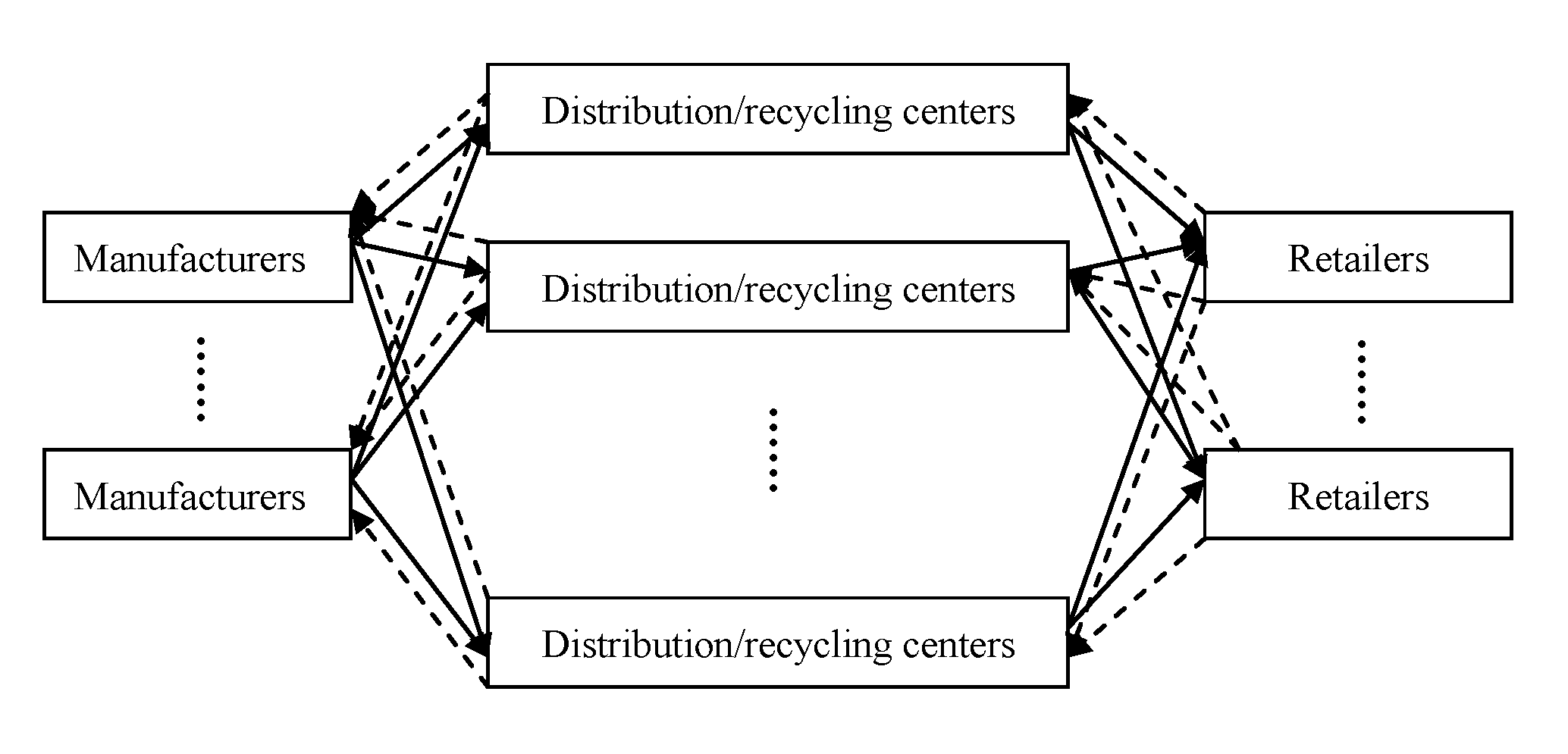
3. Model for the Forward–Reverse Logistics Network

3.1. Problem Definition and Assumptions

In this paper, a forward–reverse logistics network is considered that includes manufacturers/remanufacturers, distributors/recycling centers and retailers in the green forward–reverse logistics. The main problem is finding the optimal strategy to achieve more revenue with less environmental pollution for each firm. Hence, a multi-objective optimization model is formulated. The first objective function is to maximize total revenue, the second objective is to reduce the economic costs, and the third objective is to minimize pollution emissions.

Figure 1 presents the schematic of the forward–reverse logistics network. Two flows are considered. In the forward flow, new products are dispatched from manufacturers to distributors and then to retailers, who will ultimately send the products to consumers. In the reverse flow, recycled products are returned from retailers to distributors and then to remanufacturers, who remanufacture the recycled products. In this process, distributors play an important role in administering new/remanufactured products, distributing new/remanufactured products to retailers, collecting recycled products from retailers, determining the quality of returned products, and sending renewable recycled products to manufacturers.

The assumptions and limitations of the model are as follows.

(1)

The model represents a single period with multiple products.

(2)

No good flows exist between facilities at the same level.

(3)

The locations of manufacturing plants and distribution centers are determined.

(4)

The demand from retailers can be completely met by the distributors but are uncertain. D_k^s denotes the random demand of the kth retailer for product s and satisfies

$$P\left(D_k^s\le x\right)={\displaystyle {\int }_0^x{f}_{D_k^s}\left(t\right)dt}$$

(1)

where $f_{D_k^s}(t)dt$ is the probability density of D_k^s. $D_{k_1}^s$ and $D_{k_2}^s$ are independent when $k_1\ne k_2$.

(5)

The number of product s recycled by the kth retailer, $R_k^s$, is a random variable. $R_{k_1}^s$ and $R_{k_2}^s$ are independent when $k_1\ne k_2$.

The first three assumptions are based on the assumptions given by [21], and last two assumptions are the extended issues in this paper that consider uncertain demand and returns.

3.2. Indices

Four types of indices are considered in this paper:

i: index of manufacturing centers (manufacturers), $i\in I$;

j: index of distribution/recycling centers (distributors), $j\in J$;

k: index of retailers, $k\in K$;

s: index of products, $s\in S$.

3.3. Parameters

Table 1. Parameters of the forward–reverse logistics network model.

Parameter	Definition
Dks	Market demand for product s from the kth retailer
Djks	The jth distributor’s demand for product s from the kth retailer
$P_{ij}^s$	Price of a unit of new/remanufactured product s from the ith manufacturer to the jth distributor
$P_{jk}^s$	Price of a unit of new/remanufactured product s from the jth distributor to the kth retailer
$P_k^s$	Price of a unit of product s for the kth retailer
${\mathrm{Pr}}_{ij}^s$	Recycled price of a unit of product s from the jth distributor to the ith manufacturer
${\mathrm{Pr}}_{jk}^s$	Recycled price of a unit of product s from the kth retailer to the jth distributor
$C{n}_i^s$	Cost of producing a unit of new product s for the ith manufacturer
$C{r}_i^s$	Cost of producing a unit of remanufactured product s for the ith manufacturer
$T{c}_{ij}^s$	Cost of transacting a unit of new/remanufactured product s from the ith manufacturer to the jth distributor
$T{c}_{jk}^s$	Cost of transacting a unit of new/remanufactured product s from the jth distributor to the kth retailer
$R_k^s$	Number of product s recycled by the kth retailer
$R{c}_k^s$	Cost of a unit of recycled product s by the kth retailer
$R{c}_{ij}^s$	Cost of transacting a unit of recycled product s from the jth distributor to the ith manufacturer
$R{c}_{jk}^s$	Cost of transacting a unit of recycled product s from the kth retailer to the jth distributor
$P{c}_{1j}^s$	Cost of processing a unit of new/remanufactured product s for the jth distributor
$P{c}_{2j}^s$	Cost of processing a unit of recycled product s for the jth distributor
$Em{n}_i^s$	Amount of pollution produced by the ith manufacturer in producing a unit of new product s
$Em{r}_i^s$	Amount of pollution produced by the ith manufacturer in producing a unit of remanufactured product s
$E_{ij}^s$	Amount of pollution for a unit of new/remanufactured product s from the ith manufacturer to the jth distributor
$E_{jk}^s$	Amount of pollution for a unit of new/remanufactured product s from the jth distributor to the kth retailer
$E{r}_{ij}^s$	Amount of pollution for a unit of recycled product s from the jth distributor to the ith manufacturer
$E{r}_{jk}^s$	Amount of pollution for a unit of recycled product s from the kth retailer to the jth distributor
$a_k^s$	Initial quality of product s owned by the kth retailer
${\lambda }_{1k}^s$	Cost of inventorying a unit of product s for the kth retailer when supply exceeds demand
${\lambda }_{2k}^s$	Punishment cost per unit of product s for the kth retailer when demand exceeds supply
$\overline{Q{n}_i^s}$	The maximum quantity of new product s produced by the ith manufacturer
$\overline{Q{m}_{ij}^s}$	The maximum quantity of product s sold from the ith manufacturer to the jth distributor
$\overline{Q{d}_{ij}^s}$	The maximum quantity of product s sold from the jth distributor to the kth retailer
$g{m}_i$	Capacity of the ith manufacturer
$g{d}_j$	Capacity of the jth distributor
$g{r}_k$	Capacity of the kth retailer

shows the parameters used in this paper.

3.4. Decision Variables

Table 2. Decision variables of the forward–reverse logistics network model.

Parameter	Definition
$Q{n}_i^s$	Quality of new product s produced by the ith manufacturer.
$Q_{ij}^s$	Quality of product s sold from the ith manufacturer to the jth distributor.
$Q_{jk}^s$	Quality of product s sold from the jth distributor to the kth retailer.
$R_{ij}^s$	Quality of product s recycled from the jth recycling centers to the ith manufacturer.
$R_{jk}^s$	Quality of product s recycled from the kth recycling centers to the jth distributor.

shows the decision variables that are used in this paper.

3.5. Mathematical Model

The mathematical model can be described as follows:

$$Max{Z}_1={\displaystyle \sum _{s,i,j}{P}_{ij}^s{Q}_{ij}^s}+\left({\displaystyle \sum _{s,j,k}{P}_{jk}^s{Q}_{jk}^s}+{\displaystyle \sum _{s,i,j}{\mathrm{Pr}}_{ij}^s{R}_{ij}^s}\right)+{\displaystyle \sum _{s,k}{P}_k^{s}E(D_k^s)}$$

(2)

$$\begin{array}{cc}\hfill Min{Z}_2& =\left({\displaystyle \sum _{s,i,j}{\mathrm{Pr}}_{ij}^s{R}_{ij}^s}+{\displaystyle \sum _{s,i}C{n}_i^{s}Q{n}_i^s}+{\displaystyle \sum _{s,i,j}C{r}_i^s{R}_{ij}^s}+{\displaystyle \sum _{s,i,j}T{c}_{ij}^s{Q}_{ij}^s}\right)\hfill \\ & +\left({\displaystyle \sum _{s,i,j}{P}_{ij}^s{Q}_{ij}^s}+{\displaystyle \sum _{s,j,k}{\mathrm{Pr}}_{jk}^s{R}_{jk}^s}+{\displaystyle \sum _{s,i,j}R{c}_{ij}^s{R}_{ij}^s}+{\displaystyle \sum _{s,i,j}P{c}_{1j}^s{Q}_{ij}^s}+{\displaystyle \sum _{s,j,k}P{c}_{2j}^s{R}_{jk}^s}+{\displaystyle \sum _{s,j,k}T{c}_{jk}^s{Q}_{jk}^s}\right)\hfill \\ & +\left({\displaystyle \sum _{s,j,k}R{c}_{jk}^s{R}_{jk}^s}+{\displaystyle \sum _{s,k}R{c}_k^s\cdot E\left(R_k^s\right)}+{\displaystyle \sum _{s,k}{\lambda }_{1k}^s\cdot E\left({\Delta }_{1k}^s\right)}+{\displaystyle \sum _{s,k}{\lambda }_{2k}^s\cdot E\left({\Delta }_{2k}^s\right)}\right)\hfill \end{array}$$

(3)

$$Min{Z}_3=\left({\displaystyle \sum _{s,i}Em{n}_i^{s}Q{n}_i^s}+{\displaystyle \sum _{s,i,j}Em{r}_i^s{R}_{ij}^s}+{\displaystyle \sum _{s,i,j}{E}_{ij}^s{Q}_{ij}^s}\right)+\left({\displaystyle \sum _{s,j,k}{E}_{jk}^s{Q}_{jk}^s}+{\displaystyle \sum _{s,i,j}E{r}_{ij}^s{R}_{ij}^s}\right)+{\displaystyle \sum _{s,j,k}E{r}_{jk}^s{R}_{jk}^s}$$

(4)

Three objective functions are considered. The first objective function aims to maximize the total revenue, which consists of three terms: The first term is the revenue of the manufacturers, the second term is the expected revenue of the distributors, and the third term is the expected revenue of the retailers. The second objective function aims to minimize the total costs: The first term is the expected cost of the manufacturers, the second term is the expected cost of the distributors, and the third term is the expected cost of the retailers, where

$${\Delta }_{1k}^s=\max \left\{0,{\displaystyle \sum _j{Q}_{jk}^s}-D_k^s\right\}$$

(5)

$${\Delta }_{2k}^s=\max \left\{0,D_k^s-{\displaystyle \sum _j{Q}_{jk}^s}\right\}$$

(6)

$$E\left({\Delta }_{1k}^s\right)={\displaystyle {\int }_0^{{\displaystyle \sum _j{Q}_{jk}^s}}\left({\displaystyle \sum _j{Q}_{jk}^s-t}\right)f_{D_k^s}\left(t\right)dt}$$

(7)

$$E\left({\Delta }_{2k}^s\right)={\displaystyle {\int }_{{\displaystyle \sum _j{Q}_{jk}^s}}^{+\infty }\left(t-{\displaystyle \sum _j{Q}_{jk}^s}\right)f_{D_k^s}\left(t\right)dt}$$

(8)

The third objective function is to minimize the quantity of pollution emissions where ${\displaystyle \sum _{s,i}Em{n}_i^s{Q}_i^s}+{\displaystyle \sum _{s,i,j}Em{r}_i^s{R}_{ij}^s}+{\displaystyle \sum _{s,i,j}{E}_{ij}^s{Q}_{ij}^s}$ is the amount of pollution emissions caused by manufacturers in the course of producing and supplying products for distribution centers, ${\displaystyle \sum _{s,j,k}{E}_{jk}^s{Q}_{jk}^s}+{\displaystyle \sum _{s,i,j}E{r}_{ij}^s{R}_{ij}^s}$ is the amount of pollution emissions caused by distribution centers in supplying products for demand markets and manufacturing plants, and ${\displaystyle \sum _{s,j,k}E{r}_{jk}^s{R}_{jk}^s}$ is the amount of pollution emissions caused by demand markets in supplying recycled products for distribution/recycling centers.

The relative constraints are presented in the following equations.

$${\displaystyle \sum _j{Q}_{ij}^s}\le Q{n}_i^s+{\displaystyle \sum _j{R}_{ij}^s}\begin{array}{cc}& \forall i\end{array},s$$

(9)

$${\displaystyle \sum _k{Q}_{jk}^s}\le {\displaystyle \sum _i{Q}_{ij}^s}\begin{array}{cc}& \forall j\end{array},s$$

(10)

$${\displaystyle \sum _i{R}_{ij}^s}\le {\displaystyle \sum _k{R}_{jk}^s}\begin{array}{cc}& \forall j\end{array},s$$

(11)

$${\displaystyle \sum _j{R}_{jk}^s}\le E\left(R_k^s\right)\begin{array}{cc}& \forall k,s\end{array}$$

(12)

$$E\left(R_k^s\right)\le a_k^s+{\displaystyle \sum _j{Q}_{jk}^s}\begin{array}{cc}& \forall k,s\end{array}$$

(13)

$${\displaystyle \sum _{s,j}\left(Q_{ij}^s+R_{ij}^s\right)}\le g{m}_i\begin{array}{cc}& \forall i\end{array}$$

(14)

$${\displaystyle \sum _{s,k}\left(Q_{jk}^s+R_{jk}^s\right)}+{\displaystyle \sum _{s,i}\left(Q_{ij}^s+R_{ij}^s\right)}\le g{d}_j\begin{array}{cc}& \forall j\end{array}$$

(15)

$${\displaystyle \sum _{s,j}\left(Q_{jk}^s+R_{jk}^s\right)}\le g{r}_k\begin{array}{cc}& \forall k\end{array}$$

(16)

$$0\le Q{n}_i^s\le \overline{Q{n}_i^s}\begin{array}{cc}& \forall i\end{array},s$$

(17)

$$0\le Q_{ij}^s\le \overline{Q_{ij}^s}\begin{array}{cc}& \forall i\end{array},j,s$$

(18)

$$0\le Q_{jk}^s\le \overline{Q_{jk}^s}\begin{array}{cc}& \forall \end{array}j,k,s$$

(19)

$$R_{ij}^s,R_{jk}^s\ge 0\begin{array}{cc}& \forall \end{array}i,j,k,s$$

(20)

Constraints (9) and (10) guarantee that all the demand from distributors and retailers in the forward logistics process can be satisfied. Constraint (9) shows that, for each manufacturer, the number of products that are sold is not greater than the total number of newly manufactured products and remanufactured products recycled from recycling centers. Constraint (10) guarantees that, for each distributor, the number of products sold to retailers is not greater than the number of products received from manufacturers.

Constraints (11)–(13) limit the recycled demand of the reverse logistics system given the corresponding inputs. Constraint (11) shows that, for each distributor, the quantity of recycled products from demand markets is not less than the quantity of recycled products sent to manufacturers. Constraint (12) shows the limited capacity of each retailer to recycle products. Constraint (13) shows the limited recycled capacity of each demand market.

Constraints (14)–(16) indicate the limited storage capacity of manufacturers, distributors and retailers, respectively. Constraint (17) indicates the limited manufacturing capacity of the manufacturer for new products. Constraints (18) and (19) illustrate the limited capacity of each manufacturer and distributor, respectively. Constraint (20) presents the non-negative property of variables.

4. Solution Method

The aim of this work is to find the optimal strategy for a forward–reverse logistics network by solving a multi-objective optimization model. Then, NSGA-II is applied.

The NSGA-II method is mainly based on the genetic algorithm (GA). Generated populations are sorted by the non-dominated method [45,46]. Ranking the solutions can generate the Pareto fronts. The crowding distance and its rank can be calculated for each solution. New solutions could be generated by using mutation operators and then added to the existing population. Then, the new population can be sorted, and the system can select its size from these existing solutions [47,48]. Details on NSGA-II can be found in the works of Deb et al. [22].

NSGA-II can be used to solve generation expansion planning problems and economic power dispatch [39,40,49,50,51]. Optimal Pareto solutions and some suitable solutions can be provided for multi-objective model problems by NSGA-II, which is based on the theory of encoding chromosomes. Furthermore, based on the GA, the generated Pareto solutions are adaptive and stable. Compared with NSGA, NSGA-II is better in the sorting algorithm because it provides a fast non-dominated sorting mechanism and does not need any sharing parameters to be chosen. Moreover, NSGA-II is useful for obtaining the well-distributed Pareto fronts and a global search space.

5. Results and Discussion

Test problems for two different sizes (small and large) are considered in this section. The model is solved by using NSGA-II, which is described above.

5.1. Values of Parameters

Table 3. Parameters for different-sized firms.

	Small Firms	Large Firms
Number of manufactures (I)	1	2
Number of distributors (J)	1	2
Number of retailers (K)	2	2
Number of product types (S)	2	3

shows the values of the parameters for the sizes of firms. Note that the number of different sectors in our problem is mainly assumed based on the assumptions in [21]. Uncertain market demand, $D_k^s$, is assumed to follow a uniform distribution [0, 200/P_k^s]. $R_k^s=0.3D_k^s$, and the values of other parameters are defined as follows. Considering reality, sale prices are assumed to increase for the same product along the forward flow, while recycled costs are assumed to increase for the same product along the reverse flow. The unit costs of producing new products are slightly higher than those of producing remanufactured products for the same manufacturer.

• Sales prices of products from manufacturers to distributors.

$$\left(P_{ij}^{\left(1\right)},P_{ij}^{\left(2\right)},P_{ij}^{\left(3\right)}\right)=\left(3,4,5\right)$$

where P_ij^(s) is the sale price of new and remanufactured products from the ith manufacturer to the jth distributor for the sth product, s = 1, 2, 3.

• Sales prices of products from distributors to retailers:

$$\left(P_{jk}^{\left(1\right)},P_{jk}^{\left(2\right)},P_{jk}^{\left(3\right)}\right)=\left(5,6,7\right)$$

where P_jk^(s) is the sale price of new and remanufactured products from the jth distributor to the kth retailer for the sth product, s = 1, 2, 3.

• Sales prices of products from retailers to markets:

$$\left(\begin{array}{l}{P}_1^{\left(1\right)},P_1^{\left(2\right)},P_1^{\left(3\right)}\\ P_2^{\left(1\right)},P_2^{\left(2\right)},P_2^{\left(3\right)}\end{array}\right)=\left(\begin{array}{ccc}8& 9& 10\\ 10& 11& 12\end{array}\right)$$

where P_k^(s) is the sale price of new and remanufactured products from the kth distributor to the market for the sth product, s = 1, 2, 3.

• Prices of recycled products from distributors to manufacturers:

$$\left(\begin{array}{ccc}{\mathrm{Pr}}_{1j}^{\left(1\right)}& {\mathrm{Pr}}_{1j}^{\left(2\right)}& {\mathrm{Pr}}_{1j}^{\left(3\right)}\\ {\mathrm{Pr}}_{2j}^{\left(1\right)}& {\mathrm{Pr}}_{2j}^{\left(2\right)}& {\mathrm{Pr}}_{2j}^{\left(3\right)}\end{array}\right)=\left(\begin{array}{ccc}0.04& 0.05& 0.06\\ 0.05& 0.05& 0.04\end{array}\right),j\in J$$

where Pr_ij^(s) is the price of recycled products from the jth distributor to the ith manufacturer for the sth product, s = 1, 2, 3.

• Prices of recycled products from retailers to distributors:

$$\left(\begin{array}{ccc}{\mathrm{Pr}}_{jk}^{\left(1\right)}& {\mathrm{Pr}}_{jk}^{\left(2\right)}& {\mathrm{Pr}}_{jk}^{\left(3\right)}\end{array}\right)=\left(\begin{array}{ccc}0.02& 0.02& 0.03\end{array}\right),j\in J,k\in K$$

where Pr_jk^(s) is the price of recycled products from the k^th distributor to the jth distributor for the sth product, s = 1, 2, 3.

• Unit cost of producing new products at the manufacturer:

$$\left(\begin{array}{ccc}C{n}_1^{\left(1\right)}& C{n}_1^{\left(2\right)}& C{n}_1^{\left(3\right)}\\ C{n}_2^{\left(1\right)}& C{n}_2^{\left(2\right)}& C{n}_2^{\left(3\right)}\end{array}\right)=\left(\begin{array}{ccc}0.1& 0.08& 0.08\\ 0.08& 0.07& 0.1\end{array}\right)$$

where Cn_i^(s) is the unit-producing cost for new products at the ith manufacturer for the sth product, s = 1, 2, 3.

• Unit cost of producing remanufactured products at the manufacturer:

$$\left(\begin{array}{ccc}C{r}_1^{\left(1\right)}& C{r}_1^{\left(2\right)}& C{r}_1^{\left(3\right)}\\ C{r}_2^{\left(1\right)}& C{r}_2^{\left(2\right)}& C{r}_2^{\left(3\right)}\end{array}\right)=\left(\begin{array}{ccc}0.07& 0.05& 0.05\\ 0.05& 0.03& 0.06\end{array}\right)$$

where Cr_i^(s) is the unit-producing cost of the remanufactured products at the ith manufacturer for the sth product, s = 1, 2, 3.

• Unit transaction costs borne by manufacturers when providing the product to distributors:

$$\left(\begin{array}{ccc}T{c}_{ij}^{\left(1\right)}& T{c}_{ij}^{\left(2\right)}& T{c}_{ij}^{\left(3\right)}\end{array}\right)=\left(\begin{array}{ccc}0.01& 0.02& 0.01\end{array}\right),i\in I,j\in J$$

where Tc_ij^(s) is the unit transaction cost borne by the ith manufacturer for providing the products to the jth distributor for the sth product, s = 1, 2, 3.

• Unit transaction costs borne by the distributors for providing products to retailers:

$$\left(\begin{array}{ccc}T{c}_{jk}^{\left(1\right)}& T{c}_{jk}^{\left(2\right)}& T{c}_{jk}^{\left(3\right)}\end{array}\right)=\left(\begin{array}{ccc}0.02& 0.04& 0.02\end{array}\right),j\in J,k\in K$$

where Tc_jk^(s) is the unit transaction cost borne by the jth distributor for providing products to the kth distributor for the sth product, s = 1, 2, 3.

• The quantity of recycled products, $R_k^s$, follows a uniform distribution in [0, 10], in which $k\in K,s\in S$.

• Unit transaction costs borne by distributors for supplying recycled products to manufacturers:

$$\left(\begin{array}{ccc}R{c}_{ij}^{\left(1\right)}& R{c}_{ij}^{\left(2\right)}& R{c}_{ij}^{\left(3\right)}\end{array}\right)=\left(\begin{array}{ccc}0.01& 0.01& 0.01\end{array}\right),i\in I,j\in J$$

where Rc_ij^(s) is the unit transaction cost borne by the jth distributor for supplying recycled products to the ith manufacturer for the sth product, s = 1, 2, 3.

• Unit transaction costs borne by retailers for supplying recycled products to distributors:

$$\left(\begin{array}{ccc}R{c}_{jk}^{\left(1\right)}& R{c}_{jk}^{\left(2\right)}& R{c}_{jk}^{\left(3\right)}\end{array}\right)=\left(\begin{array}{ccc}0.008& 0.008& 0.008\end{array}\right),j\in J,k\in K$$

where Rc_jk^(s) is the unit transaction cost borne by the kth retailer for supplying recycled products to the jth distributor for the sth product, s = 1, 2, 3.

• Unit purchase costs paid by retailers for recycling products:

$$\left(\begin{array}{ccc}R{c}_1^{\left(1\right)}& R{c}_1^{\left(2\right)}& R{c}_1^{\left(3\right)}\\ R{c}_2^{\left(1\right)}& R{c}_2^{\left(2\right)}& R{c}_2^{\left(3\right)}\end{array}\right)=\left(\begin{array}{ccc}0.002& 0.003& 0.004\\ 0.003& 0.002& 0.005\end{array}\right)$$

where Rc_k^(s) is the unit purchase cost paid by the kth retailer for recycling products for the sth product, s = 1, 2, 3.

• Unit costs borne by distributors for processing new and remanufactured products:

$$\left(\begin{array}{ccc}P{c}_{1j}^{\left(1\right)}& P{c}_{1j}^{\left(2\right)}& P{c}_{1j}^{\left(3\right)}\end{array}\right)=\left(\begin{array}{ccc}0.02& 0.03& 0.03\end{array}\right),j\in J$$

where Pc_1j^(s) is the unit cost borne by the jth distributor for processing new products and remanufactured products for the sth product, s = 1, 2, 3.

• Unit costs borne by distributors for processing recycled products:

$$\left(\begin{array}{ccc}P{c}_{2j}^{\left(1\right)}& P{c}_{2j}^{\left(2\right)}& P{c}_{2j}^{\left(3\right)}\end{array}\right)=\left(\begin{array}{ccc}0.01& 0.01& 0.01\end{array}\right),j\in J$$

where Pc_1j^(s) is the unit cost borne by the jth distributor for processing recycled products for the sth product, s = 1, 2, 3.

• Amount of pollution produced by manufacturers when producing new products:

$$\left(\begin{array}{ccc}Em{n}_1^{\left(1\right)}& Em{n}_1^{\left(2\right)}& Em{n}_1^{\left(3\right)}\\ Em{n}_2^{\left(1\right)}& Em{n}_2^{\left(2\right)}& Em{n}_2^{\left(3\right)}\end{array}\right)=\left(\begin{array}{ccc}1& 1.2& 1.3\\ 0.9& 1& 1.1\end{array}\right)$$

where Emn_i^(s) is the unit amount of pollution produced by the ith manufacturer when producing new products for the sth product, s = 1, 2, 3.

• Amount of pollution produced by manufacturers when producing remanufactured products:

$$\left(\begin{array}{ccc}Em{r}_1^{\left(1\right)}& Em{r}_1^{\left(2\right)}& Em{r}_1^{\left(3\right)}\\ Em{r}_2^{\left(1\right)}& Em{r}_2^{\left(2\right)}& Em{r}_2^{\left(3\right)}\end{array}\right)=\left(\begin{array}{ccc}1& 1.2& 1.3\\ 0.9& 1& 1.1\end{array}\right)$$

where Emr_i^(s) is the unit amount of pollution produced by the ith manufacturer when producing remanufactured products for the sth product, s = 1, 2, 3.

• Amount of pollution produced by the manufacturer when supplying new or remanufactured products to distributors:

$$\left(\begin{array}{ccc}{E}_{ij}^{\left(1\right)}& E_{ij}^{\left(2\right)}& E_{ij}^{\left(3\right)}\end{array}\right)=\left(\begin{array}{ccc}1& 1& 1\end{array}\right),i\in I,j\in J$$

where E_ij^(s) is the unit amount of pollution produced by the ith manufacturer when supplying products to the jth distributor for the sth product, s = 1, 2, 3.

• Amount of pollution produced by distributors when supplying products to retailers:

$$\left(\begin{array}{ccc}{E}_{jk}^{\left(1\right)}& E_{jk}^{\left(2\right)}& E_{jk}^{\left(3\right)}\end{array}\right)=\left(\begin{array}{ccc}0.8& 1& 0.9\end{array}\right),j\in J,k\in K$$

where E_jk^(s) is the unit amount of pollution produced by the jth distributor when supplying products to the kth retailer for the sth product, s = 1, 2, 3.

• Amount of pollution produced by distributors when supplying recycled products to manufacturers:

$$\left(\begin{array}{ccc}E{r}_{ij}^{\left(1\right)}& E{r}_{ij}^{\left(2\right)}& E{r}_{ij}^{\left(3\right)}\end{array}\right)=\left(\begin{array}{ccc}1& 0.8& 1\end{array}\right),i\in I,j\in J$$

where Er_ij^(s) is the unit amount of pollution produced by the jth retailer when supplying recycled products to the ith manufacturer for the sth product, s = 1, 2, 3.

• Amount of pollution produced by retailers when supplying recycled products to distributors:

$$\left(\begin{array}{ccc}E{r}_{jk}^{\left(1\right)}& E{r}_{jk}^{\left(2\right)}& E{r}_{jk}^{\left(3\right)}\end{array}\right)=\left(\begin{array}{ccc}1& 1& 1\end{array}\right),j\in J,k\in K$$

where Er_jk^(s) is the unit amount of pollution produced by the kth retailer when supplying recycled products to the jth distributor for the sth product, s = 1, 2, 3.

• Initial quantity of products used by retailers:

$$\left(\begin{array}{ccc}{a}_1^{\left(1\right)}& a_1^{\left(2\right)}& a_1^{\left(3\right)}\\ a_2^{\left(1\right)}& a_2^{\left(2\right)}& a_2^{\left(3\right)}\end{array}\right)=\left(\begin{array}{ccc}10& 20& 10\\ 10& 10& 20\end{array}\right)$$

where a_k^(s) is the initial quantity of products used by the kth retailer for the sth product, s = 1, 2, 3.

• Unit inventory cost when supply exceeds demand for retailers:

$$\left(\begin{array}{ccc}{\lambda }_{11}^{\left(1\right)}& {\lambda }_{11}^{\left(2\right)}& {\lambda }_{11}^{\left(3\right)}\\ {\lambda }_{12}^{\left(1\right)}& {\lambda }_{12}^{\left(2\right)}& {\lambda }_{12}^{\left(3\right)}\end{array}\right)=\left(\begin{array}{ccc}0.03& 0.04& 0.03\\ 0.04& 0.05& 0.05\end{array}\right)$$

where λ_1k^(s) is the unit inventory cost when supply exceeds demand for the kth retailer for the sth product, s = 1, 2, 3.

• Unit shortage cost when demand exceeds supply for retailers:

$$\left(\begin{array}{ccc}{\lambda }_{21}^{\left(1\right)}& {\lambda }_{21}^{\left(2\right)}& {\lambda }_{21}^{\left(3\right)}\\ {\lambda }_{22}^{\left(1\right)}& {\lambda }_{22}^{\left(2\right)}& {\lambda }_{22}^{\left(3\right)}\end{array}\right)=\left(\begin{array}{ccc}0.01& 0.02& 0.01\\ 0.02& 0.03& 0.03\end{array}\right)$$

where λ_2k^(s) is the unit inventory cost when demand exceeds supply for the kth retailer for the sth product, s = 1, 2, 3.

• The upper limits of the decision variables are all set to 200 for simplicity. That is,

$$\overline{Q{n}_i^s}=\overline{Q{m}_i^s}=\overline{Q{d}_i^s}=200\hspace{1em}\left(i\in I\right)$$

• Storage capacity of manufacturers, distributors and retailers:

$$g{m}_i=150,g{d}_j=50,g{r}_k=60,\left(i\in I,j\in J,k\in K\right)$$

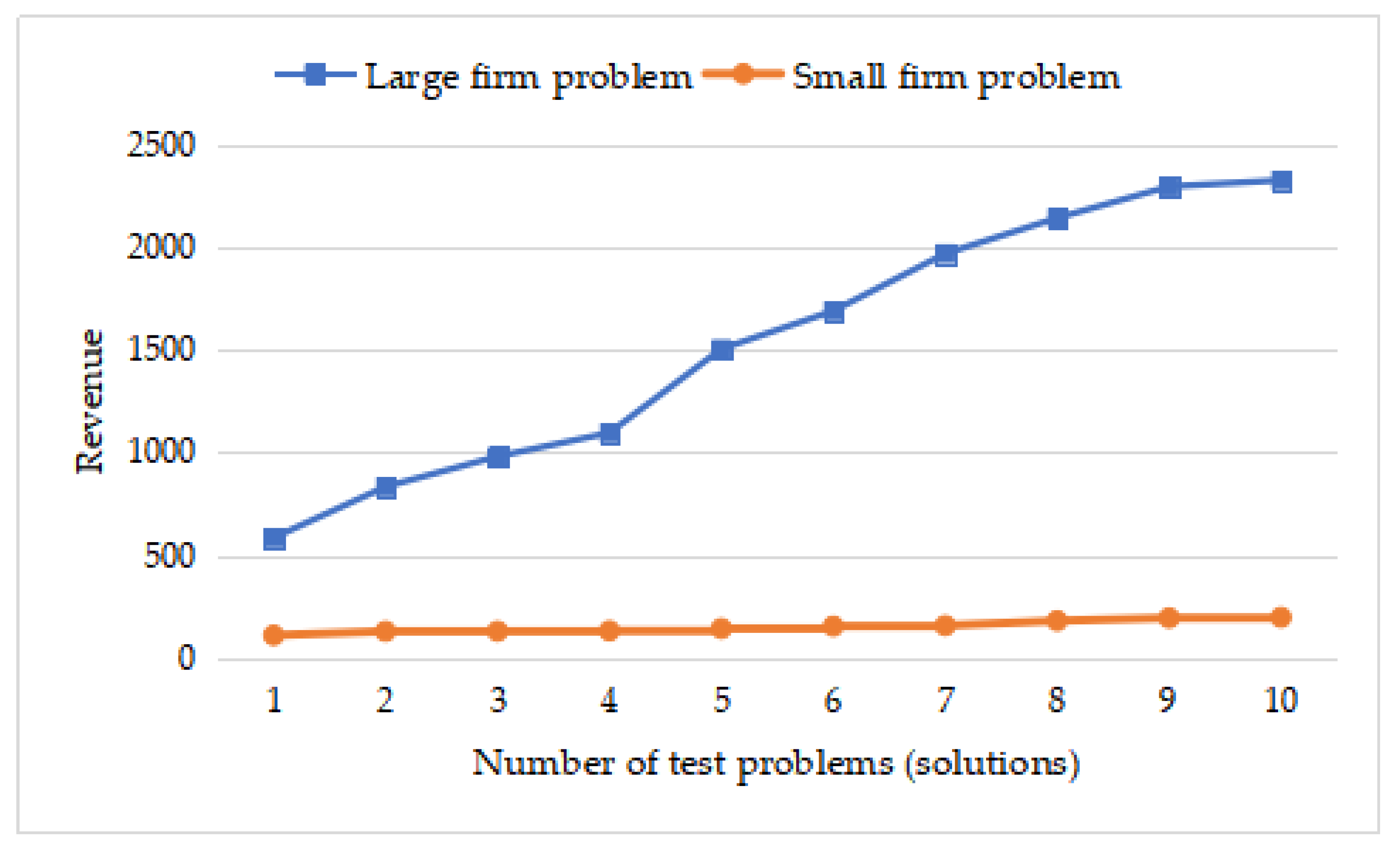
5.2. Results and Discussion

By using NSGA-II, two sets of Pareto solutions are found for firms of different sizes.

Table 4. Components of the objective values for the problem of large firms.

	Revenue	Cost	Pollution	Revenue: Cost: Pollution	Revenue/Cost
1	585.24	307.70	388.46	1.51: 0.79: 1	1.90
2	834.34	321.76	501.56	1.66: 0.64: 1	2.59
3	982.21	417.91	443.36	2.22: 0.94: 1	2.35
4	1097.57	428.13	580.02	1.89: 0.74: 1	2.56
5	1507.41	548.68	696.14	2.17: 0.79: 1	2.75
6	1693.14	652.46	668.54	2.53: 0.98: 1	2.60
7	1972.92	728.34	847.47	2.33: 0.86:1	2.71
8	2147.02	780.45	949.71	2.26: 0.82: 1	2.75
9	2300.78	828.76	1054.84	2.18: 0.79: 1	2.78
10	2331.4	846.06	861.22	2.71: 0.98: 1	2.76
Average	1545.20	586.03	699.13	2.15: 0.83: 1	2.57

and

Table 5. Components of the objective value for the problem of small firms.

	Revenue	Cost	Pollution	Revenue: Cost: Pollution	Revenue/Cost
1	108.87	38.25	42.68	2.55: 0.90: 1	2.85
2	128.16	41.40	50.30	2.55: 0.82: 1	3.10
3	128.40	41.69	51.10	2.51: 0.82: 1	3.08
4	130.42	45.54	55.58	2.35: 0.82: 1	2.86
5	141.81	44.73	57.47	2.47: 0.78: 1	3.17
6	153.26	45.92	60.50	2.53: 0.76: 1	3.34
7	156.14	47.14	64.02	2.44: 0.74: 1	3.31
8	179.62	52.98	70.80	2.54: 0.75: 1	3.39
9	193.55	57.77	81.02	2.39: 0.71: 1	3.35
10	196.37	57.54	81.49	2.41: 0.71: 1	3.41
Average	151.66	47.30	61.50	2.47: 0.78: 1	3.19

show parts of the corresponding objective values for the different problems. Figure 2 and Figure 3 illustrate the corresponding Pareto frontier for the different objective functions in the three-dimensional figures. There are 14 variables in the model for small firms and 54 variables in the model for large firms.

For large firms, Table 4 shows the components of the objective values, and Figure 2 indicates the corresponding Pareto frontier for the supply chain. Overall, the revenue function (Z₁) for the large firm problem indicates an increasing trend, where the cost function (Z₂) presents an increasing behaviour, while the values of the pollution function (Z₃) oscillate. On average, producing one unit of pollution will consume 0.83 units of cost and bring 2.15 units of revenue, and the amount of revenue brought by one unit of cost is 2.57.

For small firms, Table 5 shows components of the objective values, and Figure 3 indicates the corresponding Pareto frontier for the supply chain. Pareto solutions are closer to the ideal point in this case. With the increase in revenue (Z₁), the amount of pollution (Z₃) is increasing, while some oscillatory behaviour exists in the changes in costs (Z₂). On average, producing one unit of pollution will consume 0.78 units of cost and bring 2.47 units of revenue, and the amount of revenue brought by one unit of cost is 3.19.

Further, comparing the objective values with the average rates for the amount of revenue, cost and pollution in the last lines in Table 4 and Table 5, we find that when producing one unit of pollution, small firms will obtain more revenue and consume less cost. To compare the difference in the revenue and costs brought by one unit of pollution, we implement a variance analysis by using SPSS software at the 0.05 significance level. For the two sizes of firms, we compare the revenue brought by one unit of pollution, the costs brought by one unit of pollution, and the revenue brought by one unit of cost under a minimization condition, aiming to minimize the amount of pollution. Note that the related variables are significant at the 0.05 significance level in the normality test. The results of the variance analysis are shown in

Table 6. Results of tests on the equality of means on large and small firms.

	t-Statistic	df	sig.
Revenue brought by one unit of pollution	−2.76	9.70	0.02
Cost brought by one unit of pollution	1.32	13.93	0.21
Revenue brought by one unit of cost	−0.56	18	0.00

. For one unit of pollution, small firms can obtain significantly more revenue than large firms, while small firms consume more cost than the large firms, but the difference between the costs incurred by different sized firms is not significant at the 0.05 significance level. In addition, the value of revenue per cost is significantly larger for small firms than for large firms.

Finally, Figure 4, Figure 5 and Figure 6 describe the objective function values of the test problems. In Figure 4, the values of revenue (the first objective function) increase along with the increasing number of firms. In Figure 5, the values of cost (the second objective function) also show an increasing trend following the increasing number of firms. However, in Figure 6, there are many oscillations with an increasing number of firms for the larger firm problem, while in the small firm problem, the increasing trend is not obvious. From Figure 4, Figure 5 and Figure 6, the first and second objective functions have stable increasing behaviour as the size of the test problem increases and the number of firms increases. In addition, the behaviour of the third objective function is more erratic following the increasing number of test problems.

The above results indicate that, for multi-products and multi-sized problems, improving the value of revenue could bring greater costs and more pollution in general. That is, there are positive relationships among changes in revenue, costs and pollution amount. Different size firms have different performances When producing one unit of pollution, small firms can incur less cost and obtain more revenue. The better performance of small firms may be mainly due to their relatively concentrated production, transportation and inventory and lower costs for multi-products. However, the absolute value of the revenue obtained by large firms is much greater than that obtained by small firms. Hence, for different-sized firms, the proposed model can provide different optimal solutions.

6. Conclusions and Future Research

6.1. Conclusions

This work mainly focuses on maximizing the revenue of the system, minimizing the cost of processing and transportation, and reducing pollution emissions. A multi-objective model considering multi-stages and multi-products is proposed to optimize a green forward–reverse logistics system, thereby seeking to fill a gap in the previous research. Two economic objectives and an environmental objective are considered in forward–reverse logistics with uncertain demand and shortage costs.

The numerical results obtained by using the NSGA-II method provide Pareto-optimal solutions. Two types of problems for small and large systems are discussed. The Pareto-optimal solutions are yielded by MATLAB software for the model. We find that increasing revenue could increase cost and CO2 emissions in total. Moreover, small firms have larger revenue-cost rates and lower cost-pollution rates in the framework of minimizing the pollution emissions.

6.2. Implications for Applicability

The implication of this work is related to the study of the industry system. The results can be used by decision makers to increase the revenue, reduce total costs and reduce pollution emissions to protect the environment. Our method can also be used to help the managers of companies optimize their costs and pollution emissions throughout the forward–reverse logistics system. It would help company decision makers not only to obtain advantages in the current competitive environment but also to make plans for the future. First, more revenue can bring more pollution. Managers and governments should pay more attention to the pollution problem when they pursue higher revenue. Second, considering the pollution problem, centralized production-distribution systems have more advantages in obtaining greater revenue-cost rates and lower cost-pollution rates.

6.3. Limitations and Future Directions

We have discussed the optimization of a multi-objective decision model considering multiple products, environmental issues and uncertain demand, but there are still some shortcomings. First, we consider three objective functions: Revenue, costs and pollution emissions, and do not consider other objective functions, such as the number of machines in production and other social responsibilities. Second, our work considers the uncertainty of demand and the corresponding reward and punishment mechanisms in optimal decision making, but it lacks further analysis on the effects of these mechanisms on decision making. Third, we use two different sizes of firms as mathematical examples in a numerical analysis and determine their different performance, but the related strategic problem is too complex to be fully studied by mathematical examples. Therefore, in the future, we will consider the impact of government rewards and punishment mechanisms with more objective functions on CLSC decision making. Furthermore, we can construct more complex models and use realistic examples to give the analysis have more practical significance.

References

1. Tan, K.C.; Lyman, S.B.; Wisner, J.D. Supply chain management: A strategic perspective. Int. J. Oper. Prod. Manag. 2002, 22, 614–631. [Google Scholar] [CrossRef]
2. Zhao, X.; Huo, B.; Flynn, B.B.; Yeung, J.H.Y. The impact of power and relationship commitment on the integration between manufacturers and customers in a supply chain. Int. J. Oper. Prod. Manag. 2008, 26, 368–388. [Google Scholar] [CrossRef]
3. Su, Y.; Sun, W. Sustainability evaluation of the supply chain with undesired outputs and dual-role factors based on double frontier network DEA. Soft Comput. 2018, 22, 5525–5533. [Google Scholar] [CrossRef]
4. Giri, B.C.; Chakraborty, A.; Maiti, T. Pricing and return product collection decisions in a closed-loop supply chain with dual-channel in both forward and reverse logistics. J. Manuf. Syst. 2017, 42, 104–123. [Google Scholar] [CrossRef]
5. Accorsi, R.; Baruffaldi, G.; Manzini, R. A closed-loop packaging network design model to foster infinitely reusable and recyclable containers in food industry. Sustain. Prod. Consum. 2020, 24, 48–61. [Google Scholar] [CrossRef]
6. Tang, S.; Wang, W.; Zhou, G. Remanufacturing in a competitive market: A closed-loop supply chain in a Stackelberg game framework. Expert Syst. Appl. 2020, 161, 113655. [Google Scholar] [CrossRef]
7. Guide, V.D.R., Jr.; Van Wassenhove, L.N. Closed loop supply chains. In Quantitative Approaches to Distribution Logistics and Supply Chain Management; Springer: Berlin/Heidelberg, Germany, 2002; Volume 519, pp. 47–60. [Google Scholar] [CrossRef]
8. Min, H.; Seong Ko, C.; Jeung Ko, H. The spatial and temporal consolidation of returned products in a closed-loop supply chain network. Comput. Ind. Eng. 2006, 51, 309–320. [Google Scholar] [CrossRef]
9. Rogers, D.S.; Tibben-Lembke, R.S. Going Backwards: Reverse Logistics Trends and Practices; Reverse Logistics Executive Council: Reno, NV, USA, 1999. [Google Scholar]
10. Kumar, S.; Raut, R.D.; Narwane, V.S.; Narkhede, B.E. Applications of industry 4.0 to overcome the COVID-19 operational challenges. Diabetes Metab. Syndr. Clin. Res. Rev. 2020, 14, 1283–1289. [Google Scholar] [CrossRef]
11. Sharma, A.; Adhikary, A.; Borah, S.B. Covid-19’s impact on supply chain decisions: Strategic insights from NASDAQ 100 firms using Twitter data. J. Bus. Res. 2020, 117, 443–449. [Google Scholar] [CrossRef]
12. Majumdar, A.; Shaw, M.; Kumar Sinha, S. COVID-19 debunks the myth of socially sustainable supply chain: A case of the clothing industry in South Asian countries. Sustain. Prod. Cons. 2020, 24, 150–155. [Google Scholar] [CrossRef]
13. Govindan, K.; Mina, H.; Alavi, B. A decision support system for demand management in healthcare supply chains considering the epidemic outbreaks: A case study of coronavirus disease 2019 (COVID-19). Transp. Res. Part E Logist. Transp. Rev. 2020, 138, 101967. [Google Scholar] [CrossRef] [PubMed]
14. Hock, R.I.V. From reversed logistics to green supply chains. Supply Chain Manag. 1999, 4, 129–135. [Google Scholar] [CrossRef]
15. Su, J.; Li, C.; Zeng, Q.; Yang, J.Q.; Zhang, J. A green closed-loop supply chain coordination mechanism based on third-party recycling. Sustainability 2019, 11, 5335. [Google Scholar] [CrossRef] [Green Version]
16. Gholizadeh, H.; Fazlollahtabar, H. Robust Optimization and modified genetic algorithm for a closed loop green supply chain under uncertainty: Case study in Melting Industry. Comput. Ind. Eng. 2020, 147, 106653. [Google Scholar] [CrossRef]
17. Soleimani, H.; Chaharlang, Y.; Ghaderi, H. Collection and distribution of returned-remanufactured products in a vehicle routing problem with pickup and delivery considering sustainable and green criteria. J. Clean. Prod. 2018, 172, 960–970. [Google Scholar] [CrossRef]
18. Shi, Y.; Nie, J.; Qu, T.; Chu, L.K.; Sculli, D. Choosing reverse channels under collection responsibility sharing in a closed-loop supply chain with remanufacturing. J. Intell. Manuf. 2015, 26, 387–402. [Google Scholar] [CrossRef]
19. Soleimani, H.; Seyyed-Esfahani, M.; Kannan, G. Incorporating risk measures in closed-loop supply chain network design. Int. J. Prod. Res. 2014, 52, 1843–1867. [Google Scholar] [CrossRef]
20. El-Sayed, M.; Afia, N.; El-Kharbotly, A. A stochastic model for forward–reverse logistics network design under risk. Comput. Ind. Eng. 2010, 58, 423–431. [Google Scholar] [CrossRef]
21. Zarbakhshnia, N.; Soleimani, H.; Goh, M.; Razavi, S.S. A novel multi-objective model for green forward and reverse logistics network design. J. Clean. Prod. 2019, 208, 1304–1316. [Google Scholar] [CrossRef]
22. Deb, K.; Pratap, A.; Agarwal, S.; Meyarivan, T. A fast and elitist multiobjective genetic algorithm: NSGA-II. IEEE Trans. Evolut. Comput. 2020, 6, 182–197. [Google Scholar] [CrossRef] [Green Version]
23. Rabelo, L.; Helal, M.; Lertpattarapong, C. Analysis of supply chains using system dynamics, neural nets, and eigenvalues. In Proceedings of the 2004 Winter Simulation Conference, Washington, DC, USA, 5–8 December 2004; pp. 1136–1144. [Google Scholar] [CrossRef] [Green Version]
24. Zhou, G.; Min, H.; Gen, M. The balanced allocation of customers to multiple distribution centers in the supply chain network: A genetic algorithm approach. Comput. Ind. Eng. 2002, 43, 251–261. [Google Scholar] [CrossRef]
25. Saman, H.A. Design and Optimization of Closed-Loop Supply Chain Management. Ph.D. Thesis, Department Electrical Engineering, Windsor University, Windsor, ON, Canada, 2012. [Google Scholar]
26. Lee, J.E.; Gen, M.; Rhee, K.G. Network model and optimization of reverse logistics by hybrid genetic algorithm. Comput. Ind. Eng. 2009, 56, 951–964. [Google Scholar] [CrossRef]
27. Shi, J.; Zhang, G.; Sha, J.; Amin, S.H. Coordinating production and recycling decision with stochastic demand and return. J. Syst. Sci. Syst. Eng. 2010, 19, 385–407. [Google Scholar] [CrossRef] [Green Version]
28. Du, F.; Evans, G.W. A bi-objective reverse logistics network analysis for post-sale service. Comput. Oper. Res. 2008, 35, 2617–2634. [Google Scholar] [CrossRef]
29. Pishvaee, M.S.; Farahani, R.Z.; Dullaert, W. A memetic algorithm for bi-objective integrated forward/reverse logistics network design. Comput. Oper. Res. 2010, 37, 1100–1112. [Google Scholar] [CrossRef]
30. Fu, M.C.; Glover, F.W.; April, J. Simulation optimization: A review, new developments, and applications. In Proceedings of the 2005 Winter Simulation Conference, Orlando, FL, USA, 4 December 2005; pp. 53–61. [Google Scholar] [CrossRef]
31. Choy, K.L.; Lee, W.B.; Lo., V. Design of an intelligent supplier relationship management system: A hybrid case based neural network approach. Expert Syst. Appl. 2003, 24, 225–237. [Google Scholar] [CrossRef]
32. Giannoccaro, I.; Pontrandolfo, P.; Scozzi, B. A fuzzy echelon approach for inventory management in supply chains. Eur. J. Oper. Res. 2003, 149, 185–196. [Google Scholar] [CrossRef]
33. Vergara, F.E.; Khouja, M.; Michalewicz, Z. An evolutionary algorithm for optimizing material flow in supply chains. Comput. Ind. Eng. 2002, 43, 407–421. [Google Scholar] [CrossRef] [Green Version]
34. Zhu, Q.; Sarkis, J. Relationships between operational practices and performance among early adopters of green supply chain management practices in Chinese manufacturing enterprises. J. Oper. Manag. 2004, 22, 265–289. [Google Scholar] [CrossRef]
35. Jiao, Z.; Ran, L.; Zhang, Y.; Li, Z.; Zhang, W. Data-driven approaches to integrated closed-loop sustainable supply chain design under multi-uncertainties. J. Clean. Prod. 2018, 185, 105–127. [Google Scholar] [CrossRef]
36. Su, Y.; Sun, W. Analyzing a closed-loop supply chain considering environmental pollution using the NSGA-II. IEEE Trans. Fuzzy Syst. 2019, 27, 1066–1074. [Google Scholar] [CrossRef]
37. Su, Y.; Li, T. Simulation Analysis of Knowledge Transfer in a Knowledge Alliance Based on a Circular Surface Radiator Model. Complexity 2020, 2020, 4301489. [Google Scholar] [CrossRef]
38. Rabbani, M.; Alamdar, S.F.; Heydari, J. Pricing, collection, and effort decisions with coordination contracts in a fuzzy, three-level closed-loop supply chain. Expert Syst. Appl. 2018, 104, 261–276. [Google Scholar] [CrossRef]
39. Khalili-Damghani, K.; Abtahi, A.R.; Tavana, M. A new multi-objective particle swarm optimization method for solving reliability redundancy allocation problems. Reliab. Eng. Syst. Saf. 2013, 111, 58–75. [Google Scholar] [CrossRef]
40. Quariguasi Frota Neto, J.; Walther, G.; Bloemhof, J.A.E.E.; Van Nunen, J.A.E.E.; Spengler, T. From closed-loop to sustainable supply chains: The WEEE case. Int. J. Prod. Res. 2010, 48, 4463–4481. [Google Scholar] [CrossRef] [Green Version]
41. Ferrer, G.; Swaminathan, J.M. Managing new and remanufactured products. Manag. Sci. 2006, 52, 15–26. [Google Scholar] [CrossRef] [Green Version]
42. Zhang, L.; Wang, J.; You, J. Consumer environmental awareness and channel coordination with two substitutable products. Eur. J. Oper. Res. 2015, 241, 63–73. [Google Scholar] [CrossRef]
43. Giovanni, P.D. Environmental collaboration in a closed-loop supply chain with a reverse revenue sharing contract. Ann. Oper. Res. 2011, 220, 135–157. [Google Scholar] [CrossRef]
44. Guide, V.D.R., Jr.; Van Wassenhove, L.N. The evolution of closed-loop supply chain research. Oper. Res. 2009, 57, 10–19. [Google Scholar] [CrossRef]
45. Chen, J.M.; Chang, C.I. Dynamic pricing for new and remanufactured products in a closed-loop supply chain. Int. J. Prod. Econ. 2013, 146, 153–160. [Google Scholar] [CrossRef]
46. Vorasayan, J.; Ryan, S.M. Optimal price and quantity of refurbished products. Prod. Oper. Manag. 2006, 15, 369–383. [Google Scholar] [CrossRef]
47. Seuring, S.; Müller, M. From a literature review to a conceptual framework for sustainable supply chain management. J. Clean. Prod. 2008, 16, 1699–1710. [Google Scholar] [CrossRef]
48. Souza, G.C. Closed-loop supply chains: A critical review, and future research. Decis. Sci. 2013, 44, 7–38. [Google Scholar] [CrossRef]
49. Murugan, P.; Kannan, S.; Baskar, S. NSGA-II algorithm for multiobjective generation expansion planning problem. Electr. Power Syst. Res. 2009, 79, 622–628. [Google Scholar] [CrossRef]
50. Liu, D.; Huang, Q.; Yang, Y.; Liu, D.; Wei, X. Bi-objective algorithm based on NSGA-II framework to optimize reservoirs operation. J. Hydrol. 2020, 585, 124830. [Google Scholar] [CrossRef]
51. Bellaaj Kchaou, O.; Garbaya, A.; Kotti, M.; Pereira, P.; Fakhfakh, M.; Helena Fino, M. Sensitivity aware NSGA-II based Pareto front generation for the optimal sizing of analog circuits. Integration 2016, 55, 220–226. [Google Scholar] [CrossRef]
Figure 1. Structure of the forward–reverse logistics supply chain (the solid arrow is the forward logistics, and the dotted arrow is the reverse logistics).
Sustainability 12 06082 g001
Figure 2. Pareto frontier for the supply chain in large firms.
Sustainability 12 06082 g002
Figure 3. Pareto frontier for the supply chain in small firms.
Sustainability 12 06082 g003
Figure 4. Revenues for different-sized problems.
Sustainability 12 06082 g004
Figure 5. Costs for different sized firm problems.
Sustainability 12 06082 g005
Figure 6. Pollution emissions for different sized firm problems.
Sustainability 12 06082 g006