Article

Analysis of Potential Shift to Low-Carbon Urban Travel Modes: A Computational Framework Based on High-Resolution Smartphone Data

by
Mehrdad Bagheri
1,2,*,
Miloš N. Mladenović
1,
Iisakki Kosonen
1 and
Jukka K. Nurminen
3
1
Department of Built Environment, Aalto University, 02150 Espoo, Finland
2
Department of Computer Science, Aalto University, 02150 Espoo, Finland
3
Department of Computer Science, University of Helsinki, 00560 Helsinki, Finland
*
Author to whom correspondence should be addressed.
Sustainability 2020, 12(15), 5901; https://doi.org/10.3390/su12155901
Submission received: 24 June 2020 / Revised: 10 July 2020 / Accepted: 13 July 2020 / Published: 22 July 2020
(This article belongs to the Section Sustainable Transportation)

Abstract

:
Given the necessity to understand the modal shift potentials at the level of individual travel times, emissions, and physically active travel distances, there is a need for accurately computing such potentials from disaggregated data collection. Despite significant development in data collection technology, especially by utilizing smartphones, there are limited efforts in developing useful computational frameworks for this purpose. First, development of a computational framework requires longitudinal data collection of revealed travel behavior of individuals. Second, such a computational framework should enable scalable analysis of time-relevant low-carbon travel alternatives in the target region. To this end, this research presents an open-source computational framework, developed to explore the potential for shifting from private car to lower-carbon travel alternatives. In comparison to previous development, our computational framework estimates and illustrates the changes in travel time in relation to the potential reductions in emission and increases in physically active travel, as well as daily weather conditions. The potential usefulness of the framework was evaluated using long-term travel data of around a hundred travelers within the Helsinki Metropolitan Region, Finland. The case study outcomes also suggest that in several cases traveling by public transport or bike would not increase travel time compared to the observed car travel. Based on the case study results, we discuss potentially acceptable travel times for mode shift, and usefulness of the computational framework for decisions regarding transition to sustainable urban mobility systems. Finally, we discuss limitations and lessons learned for data collection and further development of similar computational frameworks.

1. Introduction

One of the essential measures for enabling transition to sustainable urban mobility systems is modal shift [1,2]. Here, essential factors to take into account for understanding modal shift potential are reducing emissions and increasing physical activity for individual travelers [3,4]. However, the potential shift away from passenger car use has to account for constrained daily travel time budget and activity space [5,6]. Specifically, understanding potential for modal shift requires comparing travel times of alternative modes for individual travelers, as they can influence travelers’ decisions [7]. From the standpoint of steering sustainability transitions, understanding the potential for modal shift by taking into account changes in travel time, carbon emissions, and physical activity is important for large infrastructural investments, such as public transport network overhauls [8], or for piloting new mobility services and policy programs [9,10,11,12]. For guiding these efforts, previous research informs us that comparatively longer trip duration with public transport (PT) or cycling with reference to driving is a frequent barrier for modal shift [13,14,15,16]. In contrast, there is an objective potential that some urban driving trips could be replaced with low-carbon and active modes without compromising much travel time [17,18]. Moreover, we have to recognize the importance of perceived travel time, as it can often be underestimated for driving [19], or overestimated for using PT and cycling [20]. Being able to accurately understand the potential for modal shift can also inform the development of strategies for improving users’ travel competence, and thus influence the likelihood of considering alternative travel modes [14,20,21].
Understanding the potential for modal shift at the individual level has relied on revealed-preference household questionnaires for several decades [22]. These traditional survey methods are nowadays facing a challenge in declining response rates, especially among young adults [23,24]. There are also other inherent challenges for questionnaire methods, such as resource intensity, especially for longitudinal data collection, and data quality level due to respondent errors [25,26]. In addition, it is often difficult to capture complete door-to-door travel modes using these traditional methods [27]. Responding to these challenges, there is an ongoing development of new technologies to automate and facilitate disaggregate data collection, such as GPS devices [25,28,29], cellular-network positioning from call and activity data [30,31,32], and smartphone sensors [33,34,35,36,37].
Due to smartphone use by a wider population, their sensors and processing can enable automatic collection of individual and longitudinal high-resolution travel data. In particular, smartphone-based travel data collection has the potential to cover large geographic areas, include large numbers of diverse participants, and also interact with the user through mobile apps, or combine with travel surveys, to provide additional socioeconomic, attitudinal, and contextual information [35,38,39,40,41,42]. Contrary to these potentials, this automatic detection technology also comes with challenges regarding accuracy and precision. To address these challenges, previous technological development has focused on several aspects, such as locational accuracy [43,44,45], identifying trip segments and door-to-door trips [46,47,48], as well as classification of transport modes [49,50]. Further developments of automatic post-processing of the collected data [51,52] and open-source platforms [51,53] have contributed to a wider spread and customization of smartphone-based data collection in the recent years. Finally, the recent review explains integration of smartphone-based data into the transport planning and policy methods [54].
Given the need to understand the potential for modal shift at the level of individual travel times, emissions, and physical activity, there is a need for accurately computing such potential from disaggregated data collection [55,56,57]. Along with technological trends, development of such computational frameworks for understanding latent trips has previously relied on the use of traditional travel surveys [17,18,58,59]. In contrast, developing a computational framework based on smartphone data has proved to provide more accurate measurement of the observed traveled distances, leading to better estimation of potential emissions reductions with computed alternatives [56,57]. In addition, the use of smartphone data has been shown to provide a better estimation of observed walking for PT access/egress, leading to better estimations of potential changes in physical activity with mode shift [27,60,61]. Despite these computational potentials, most of the previous literature has studied the reduced emissions and increased travel times separately [55,62], focusing on comparing alternatives such as bike, PT, or shared bike [18,63].
The above background implies two main gaps for developing a computational framework aiming at understanding potential for modal shift taking into account door-to-door travel times, carbon emissions, and physical activity with alternative travel modes. First, development of such a computational framework requires longitudinal data collection of revealed travel behavior of individuals. Second, such a computational framework should provide useful and scalable analysis for exploring time-relevant low-carbon travel alternatives in the target region. To this end, this research presents further development in the formulation and implementation of such a computational framework, expanding from Bagheri et al. [55]. The computational framework is based on high-resolution smartphone-based travel data and evaluated using a case in the Helsinki Metropolitan Region (HMR), Finland. Given this aim, the paper is organized as follows. Section 2 explains the developed open-source computational framework. Section 3 describes the setup for long-term data collection in the HMR, including a description of the validity of the collected travel data for the purpose of testing the computational framework. Section 4 shows the application of the developed computational framework to the HMR dataset. Section 5 presents a discussion of the findings and provides suggestions for further development, thus concluding the paper.

2. Computational Framework

The present paper extends the framework proposed by Bagheri et al. [55], using longitudinal data collection of revealed travel behavior of individuals for exploring the potential for shifting to low-carbon travel alternatives in a target urban region. In comparison to previous development, this current, extended, computational framework analyzes changes in travel time together with emission reductions and physically active travel, by considering variable time-increase thresholds. In addition, the new framework evaluates the parameters by person-day and presents the changes in total daily travel times (TDTs). Finally, the framework also includes real-time weather context and its influence on cycling. Table 1 summarizes the components and parameters of this computational framework. The source code of the framework is available online at https://github.com/mehrdad-bm/mobility_shift.

2.1. Data Collection and Filtering of Trip Ddata

Travel data collection is performed by using an open-source Java-based smartphone app, evaluated by Rinne et al. [45]. Participants voluntarily install the app, allowing it to automatically record travel points in the background, over extensive periods of time. Anonymous real-time movement data being collected includes point-data from GPS, accelerometer, and other phone sensors, by using Google’s Fused Location Provider API and Activity Recognition API [64,65]. The app itself does initial filtering of collected data for accuracy, discarding sample points that have an estimated accuracy worse than 50 m. Data is centrally collected on a web server. Data on the server is further processed to distinguish single-mode trip legs, including their start and end times and origin and destination geolocations [46,50,66]. The framework then detects multimodal door-to-door trips by first sorting the legs by their departure time and then connecting the consecutive legs belonging to the same multimodal trip, considering a maximum idle time threshold between legs [32]. Such a door-to-door trip in the Helsinki region would be for example: walk → bus → tram → walk. Our computational framework, implemented in Python and PostgreSQL, uses these stored database records. First, a filtering process selects only the trips viable for further analysis. This filtering aims to identify and reject incorrectly detected trips (e.g., erroneous or missing data). Correctly recorded urban trips are assumed to have average trip speed >3 km/h (minimum walk speed) and < 150 km/h (max city train speed), as also similarly considered in previous literature (Safi et al. 2016). In addition, the filtering process discards non-stop circular trips, such as running exercises, where such trips start and end at the same geolocation. Additional details on data collection and filtering have been discussed in Bagheri et al. [55] and Rinne et al. [45]. Further details about accuracy and noise in the data collection, informed by the findings of the case study, are also discussed in the discussion section of this paper.

2.2. Computing Alternative Trips

After the filtering process, the framework computes alternative trips with different low-carbon transport modes for all observed door-to-door trips. The framework computes trips with the same start time, date, origin, and destination as the original trip, but with the target alternative modes. For this purpose, we utilize OpenTripPlanner (OTP), a recognized open-source journey planning software [67], together with city open-data that includes PT routes and schedules. OTP is also used, for example, by Helsinki Region Transport (HSL) for Reittiopas, their online trip planning portal [68]. With this approach, we make sure that the computed potential alternative trip is actually possible. Modes that are considered an alternative to car driving are PT (commuter train, metro, bus, and tram), bike, and walk, while the computed alternative trip can also be multimodal (e.g., walk → bus → train → walk). For access–egress legs to/from PT stops, we assume a maximum of 1 km walking distance. The computational framework uses HTTP protocol with Representational State Transfer (REST) to send routing requests to the OTP server designated for the Helsinki region [69]. OTP returns data of the computed door-to-door trip for each requested transport mode, including all trip legs, with geolocations and timestamps. The returned data for potential trips are stored for further quantification in the next steps of the computational framework.

2.3. Quantifying Trip Attributes

After having observed and computed trips, the framework estimates per-leg and per-trip traveled distances, travel times, and carbon emissions for both. Travel time is calculated by subtracting departure/arrival times. Traveled distance is estimated by summing up lengths of segments between consecutive GPS points along the leg. Next, carbon emission is estimated based on the traveled distance, and the average carbon emission and passenger occupancy of each mode. Emission per trip leg of traveler (eleg) is calculated as (Equation (1)):
eleg = dleg × evkt ÷ o
where dleg is the distance traveled along the leg; evkt is tailpipe emission per vehicle-km traveled (vkt) depending on the transport mode; and o is passenger occupancy, i.e., average passengers per vehicle depending on the mode [70]. Values of evkt and o can vary among cities depending on transport vehicles and passenger volume. For our case study region, we get the values of evkt and o from local statistics of Finland provided by LIPASTO Unit Emissions Database [71]. According to this source, evkt of tram, metro, and city-train is zero. On average there are o = 1.7 passengers in each private car and o = 18 passengers on each city bus vehicle based on 2016 statistics. Vehicle emission is evkt = 151 g-CO2/km for a private car and evkt = 939 g-CO2/km for a city bus.

2.4. Changes in Travel Time and Its Relation to Emission Reduction and Physically Active Distance

At this phase, we select only those alternatives that show to reduce carbon emission compared to the original observed trips. For many observed trips, multiple lower-carbon alternative modes are possible. Naturally, other trip attributes such as travel times and physically active distances would also change as a result of change in modes and/or travel distance compared to the observed trips. The framework calculates these differences to get an estimation of travel time decrease/increase, emission reductions, and increased physically active distances. In order to enable per-day analysis of the potential mode shift, we calculate the total daily travel times (TDTs) per person-day, that is, sum of travel times of each traveler per day for a given transport mode. Having obtained the above information, the framework performs comparative analysis of all lower-carbon alternatives versus observed trips. Some previous works consider a small or zero threshold for travel time increase (e.g., maximum three minutes) for an alternative to be considered [18,55]. However, this research extends previous efforts by first disregarding the fixed threshold condition and evaluating all lower-carbon alternatives, comparing the associated travel time change in relation to emission reduction and increased physically active distance. Time change is presented as the amount of increased/decreased travel time in minutes as a result of potential modal shift. Furthermore, we can classify alternative trips as “feasible” and “non-feasible” according to their associated travel time change. Potential alternative trips are considered feasible when travel time increase is not more than an assumed threshold value. We pick a range of values for this time-increase threshold variable, and visualize the outcomes. As an example, the following Table 2 shows one of the cases where shifting from car to PT does not result in a significant travel time increase. Trip origin is in the Kallio neighborhood in Helsinki, and destination is in the Tuomarila neighborhood in Espoo, while departure time is 21:00 and date is Wednesday, 9 August 2017. From this example, one can conclude that the computed PT alternative has almost the same travel time as traveling by car.

2.5. Weather Context and Its Influence on Physically Active Travel

Finally, our computational framework also takes into account the weather context and its influence on physically active travel. When planning their daily activity schedule and modes, adverse weather conditions can negatively influence low-carbon mode choice of travelers. Our computational framework uses data on the average daily temperature and total daily precipitation for computing alternative biking trips. As one of the evaluation cases, the computation discards bike alternatives on days with average temperature below 10 °C, as well as days with total precipitation more than 5 mm. Real-time hourly weather information is retrieved from the open data portal of the Finnish Meteorological Institute (FMI) [72] and then aggregated per day. These values can be adjusted based on the case study region, also by evaluating the distribution of observed mode choices in relation to historical weather data.

3. Case Study Data

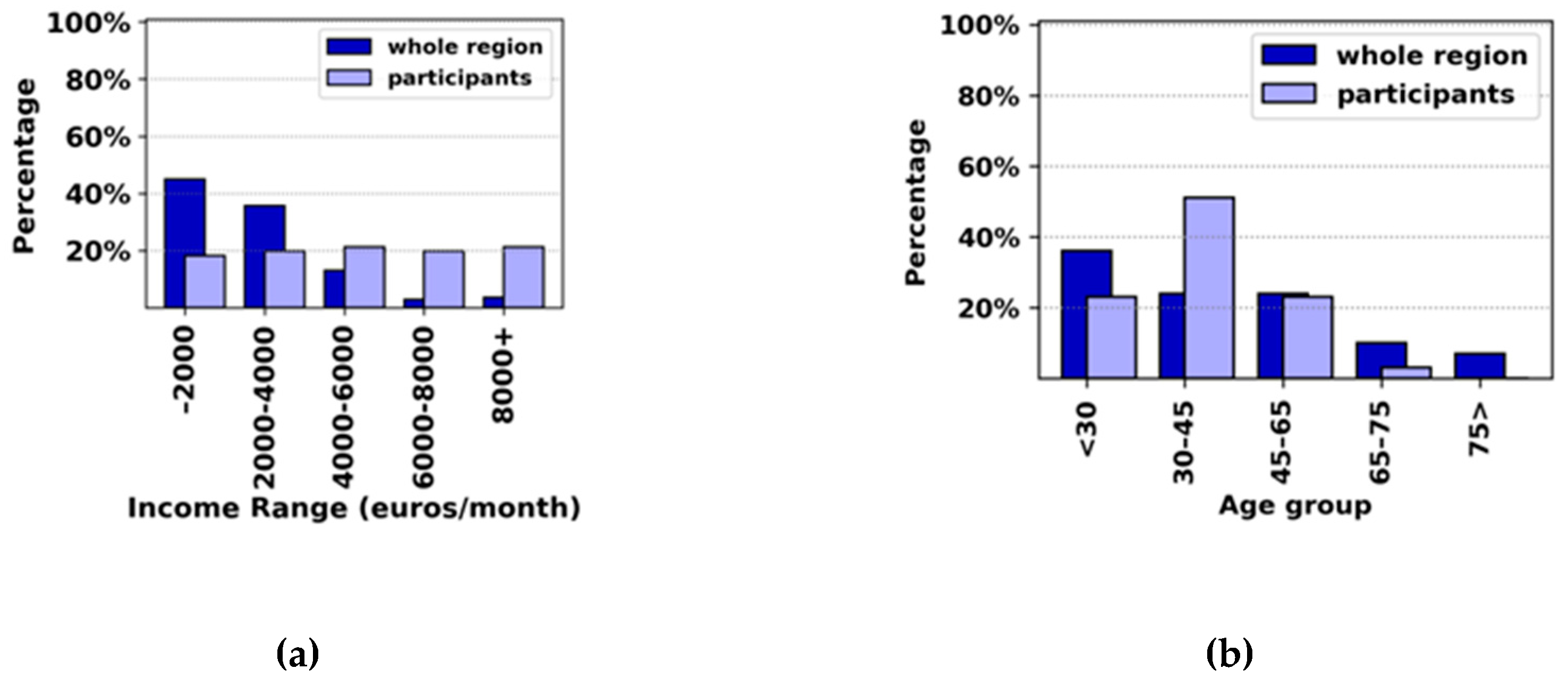
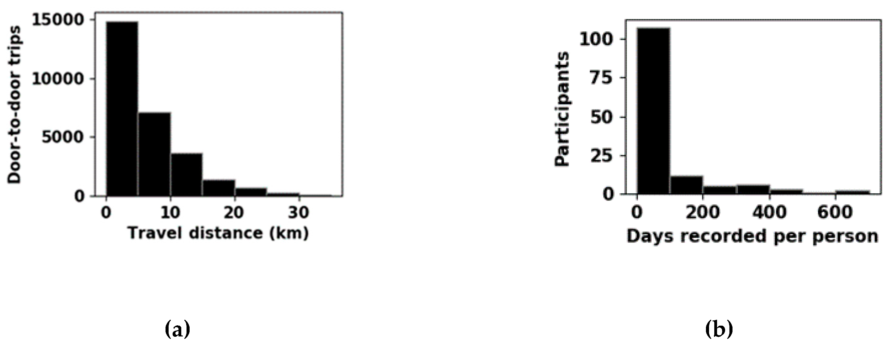
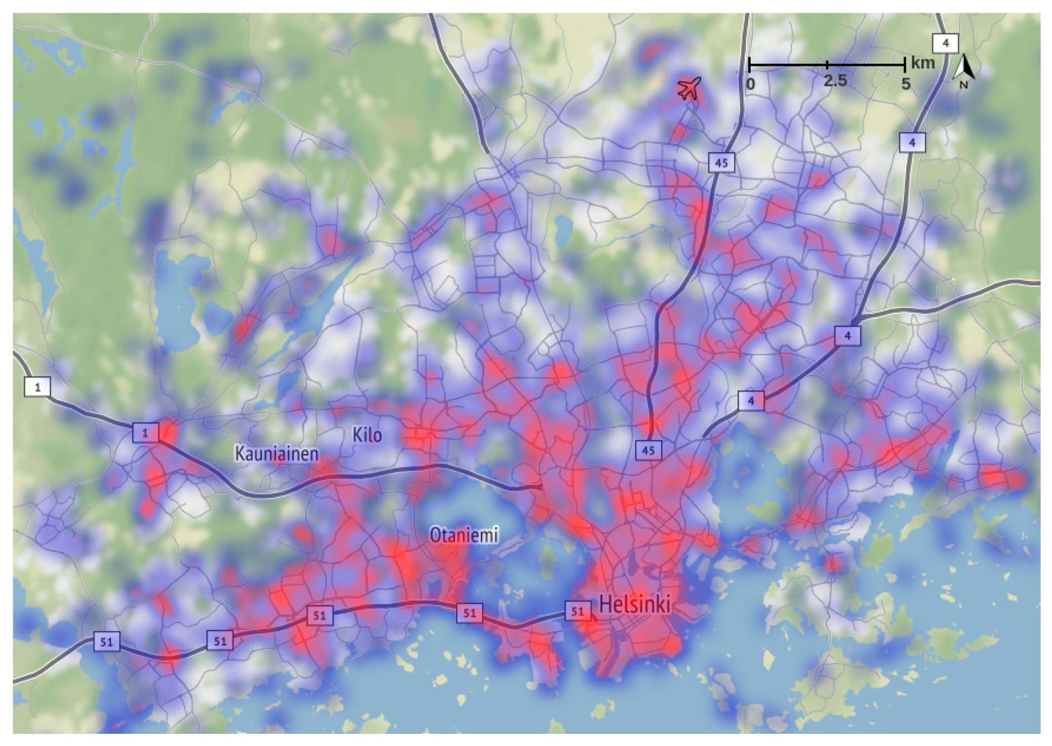
For evaluation of this framework we used the longitudinal smartphone-based travel data collected in HMR for more than three years since 2016. For testing this computational framework, we used the data collected until the end of March 2019. Volunteer recruitment relied on online advertisements and usage of social media, including two prize lotteries. There were in total 137 participants that installed the data collection app, from which 69 participants also submitted an optional online questionnaire linked in the app to provide information on their socio-demographic background. After preprocessing and refining the recorded data in our framework, the database contained more than 28,000 observed door-to-door trips, amounting to a total of more than 10,000 person-days. The following figures show the aggregate statistics of the data sample, for validation purposes. Figure 1 shows observed trips per month, day, and hour. Relative peaks in April and May are the result of a focused three-month promotion pilot in 2017. Figure 2 shows age and income distribution of study participants in relation to that of the whole HMR, showing the dominance of middle-aged participants, although there were participants in other age groups (Statistical Yearbook of Helsinki 2018). Figure 3a shows the range of traveled distances per trip, and Figure 3b shows the range of days recorded per participant, with an average value of 76 days. Figure 4 illustrates the spatial distribution of the observed trips. The map shows lower trip origin/destination density with blue color and higher density with red color. The collected data has a good spatial coverage across the HMR, as trip origins and destinations are spread around the adequate land use (e.g., housing, commercial).
Here we also compare the total daily travel times (TDTs) based on the observed trips with the daily travel times reported in daily time use surveys of the case study region [73]. There were around 10,000 observed person-days in the collected case data. The mean observed TDT in the collected case data is 53 min, while the mean reported TDT is 56 min for the whole of Finland, showing validity of data in this dimension. In addition, Figure 5 shows the range and distribution of TDT as well as the number of daily observed trips per person-day. The data show adequate distribution, resembling distributions often observed in such urban mobility datasets [74].
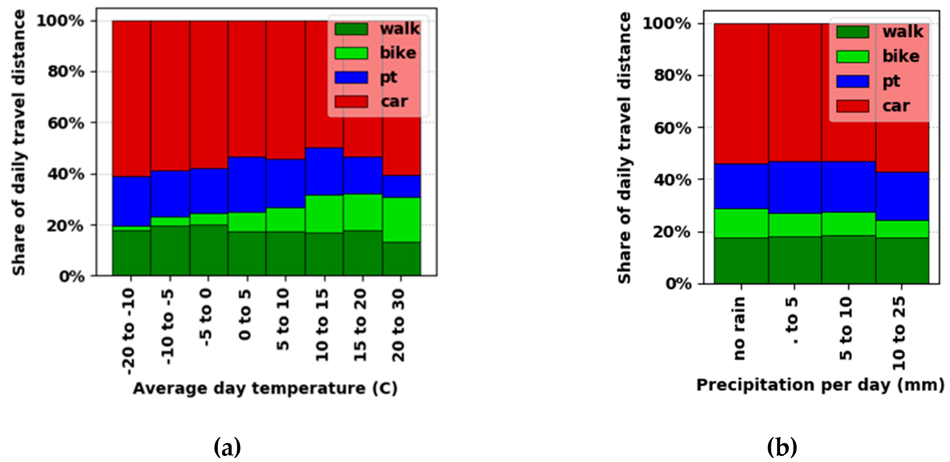
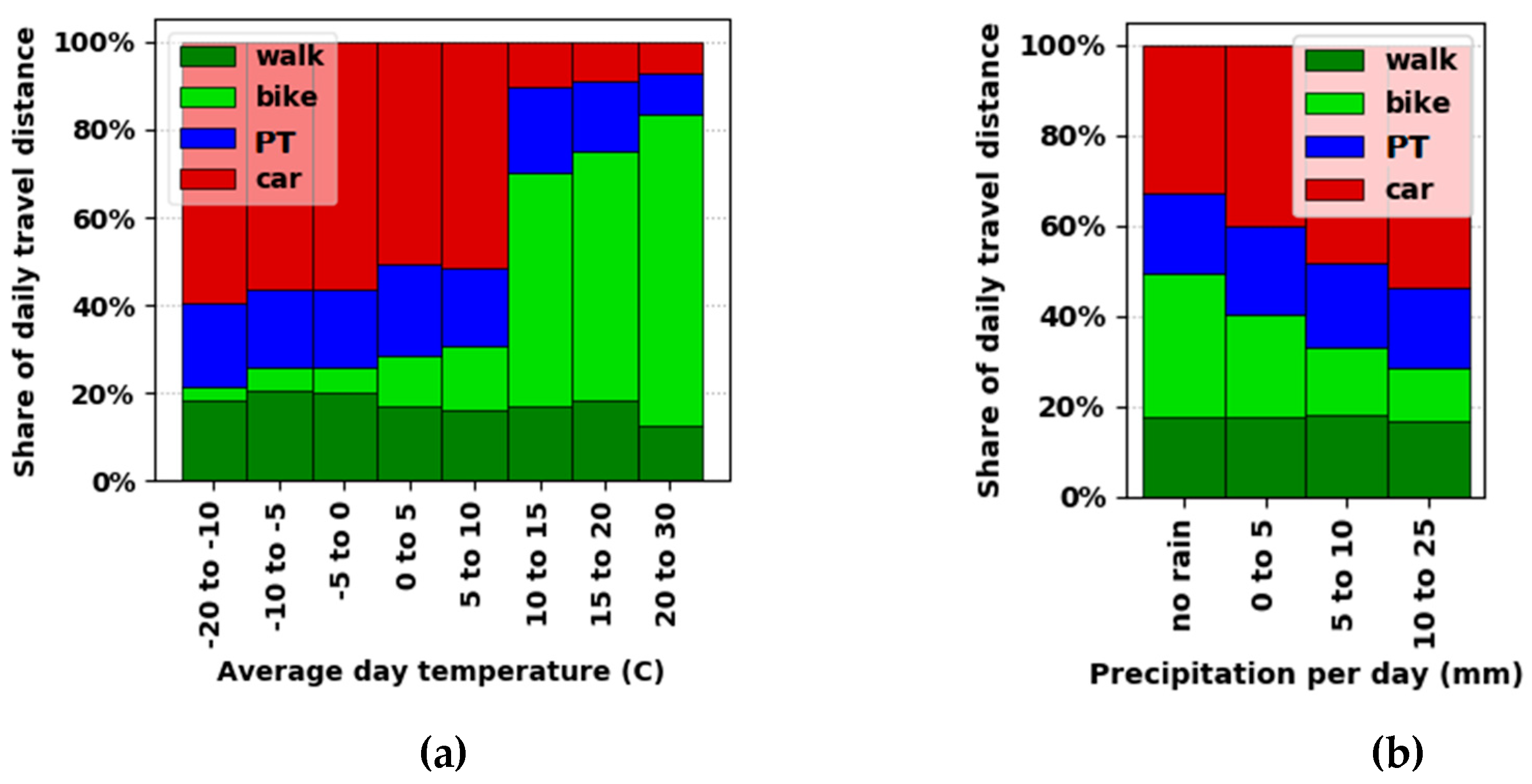
Here we review the weather condition during the data collection period and its potential correlation to daily mode choices. Figure 6 shows days of the year compared with observed trip person-days, as grouped by average day temperature and total precipitation. The figure indicates that the observed trips were distributed throughout all temperature and precipitation ranges typically observed in the case study region. In addition, this figure indicates that trip data during the case study has been collected in a relative proportion to weather data over the same period. Figure 7 shows an overview of mode choices per day and the share of physically active travel distances in relation to temperature and precipitation. One can see that bike usage had an upwards trend with increasing temperatures, and that the share of bike distance per person-day doubled, tripled, and quadrupled (from 4% to 15%) from each temperature range to another. In contrast, the share of walk distance per person-day did not change much, staying around 20%, while PT use declined a bit above 5 °C. Finally, car use declined a little above −5 °C from 36% to 30%, while the average was 33%. Precipitation showed less clear trends when compared to temperature, as precipitation levels in the Helsinki region are not high, relatively speaking. For example, only 1% of observed trip days were recorded when daily precipitation was more than 20 mm. However, car driving increased with the increase in daily precipitation, which might have important implications for computing alternative trips.

4. Case Study Results

4.1. Summative Potential Changes with Lower-Carbon Alternatives

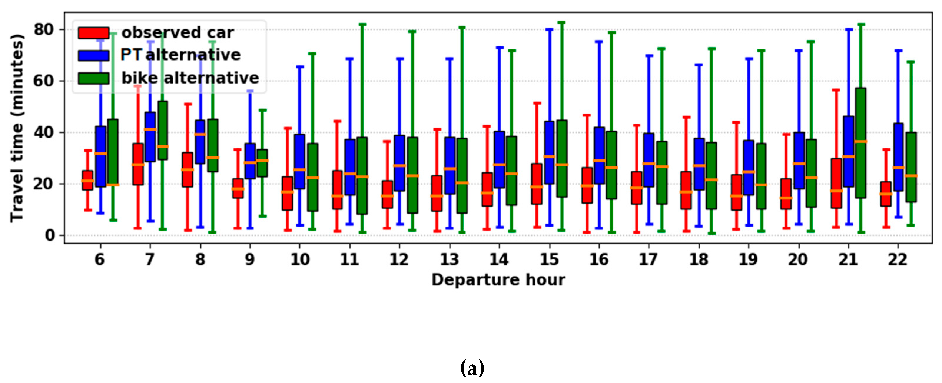
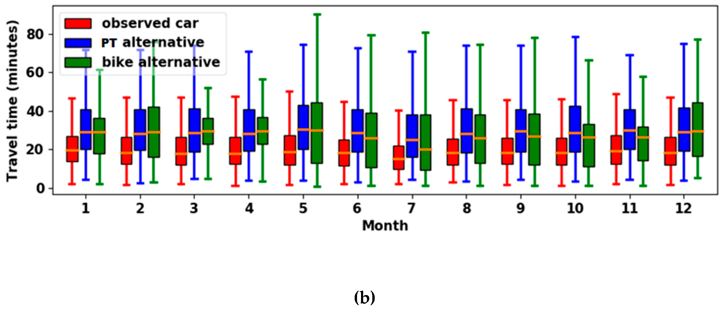
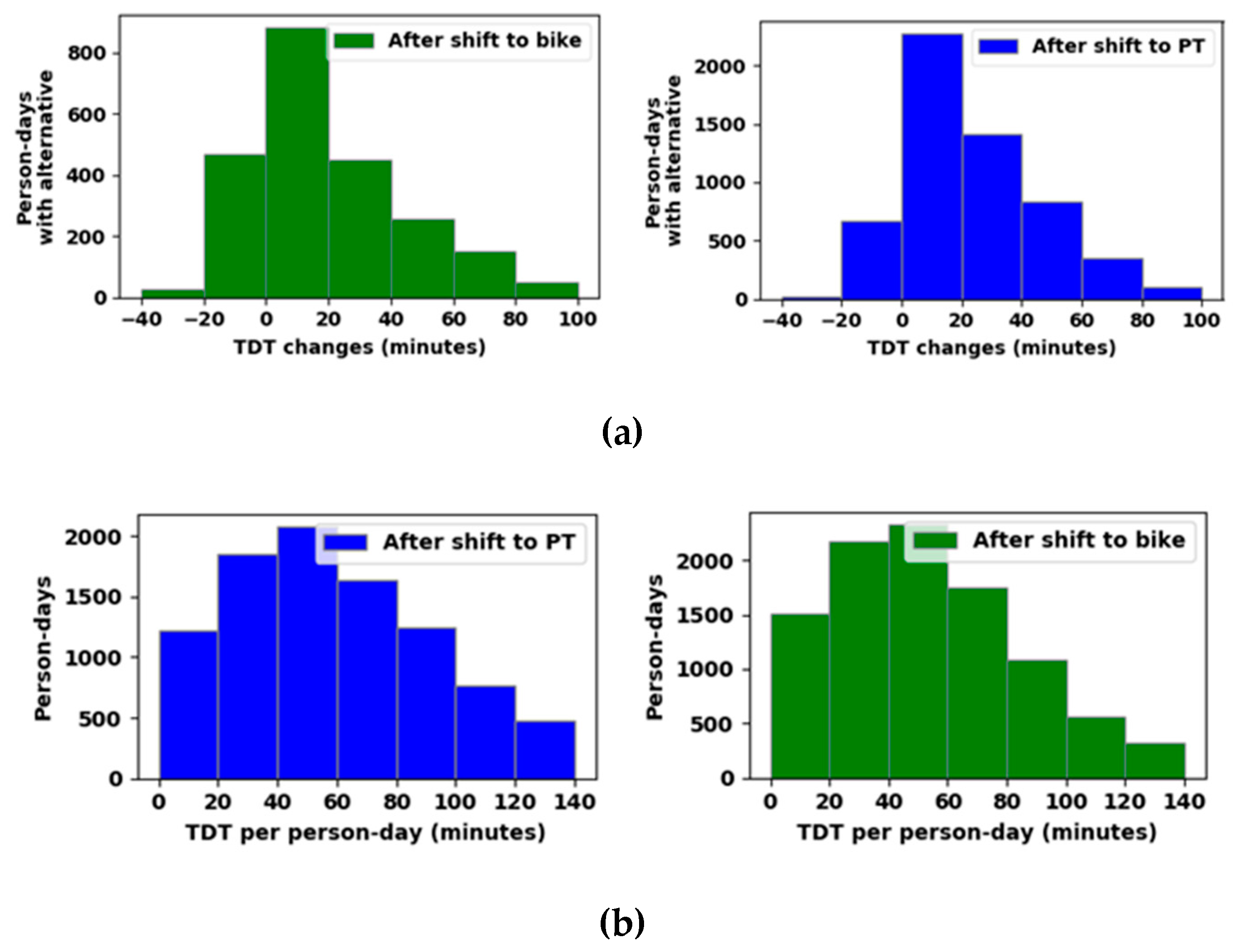
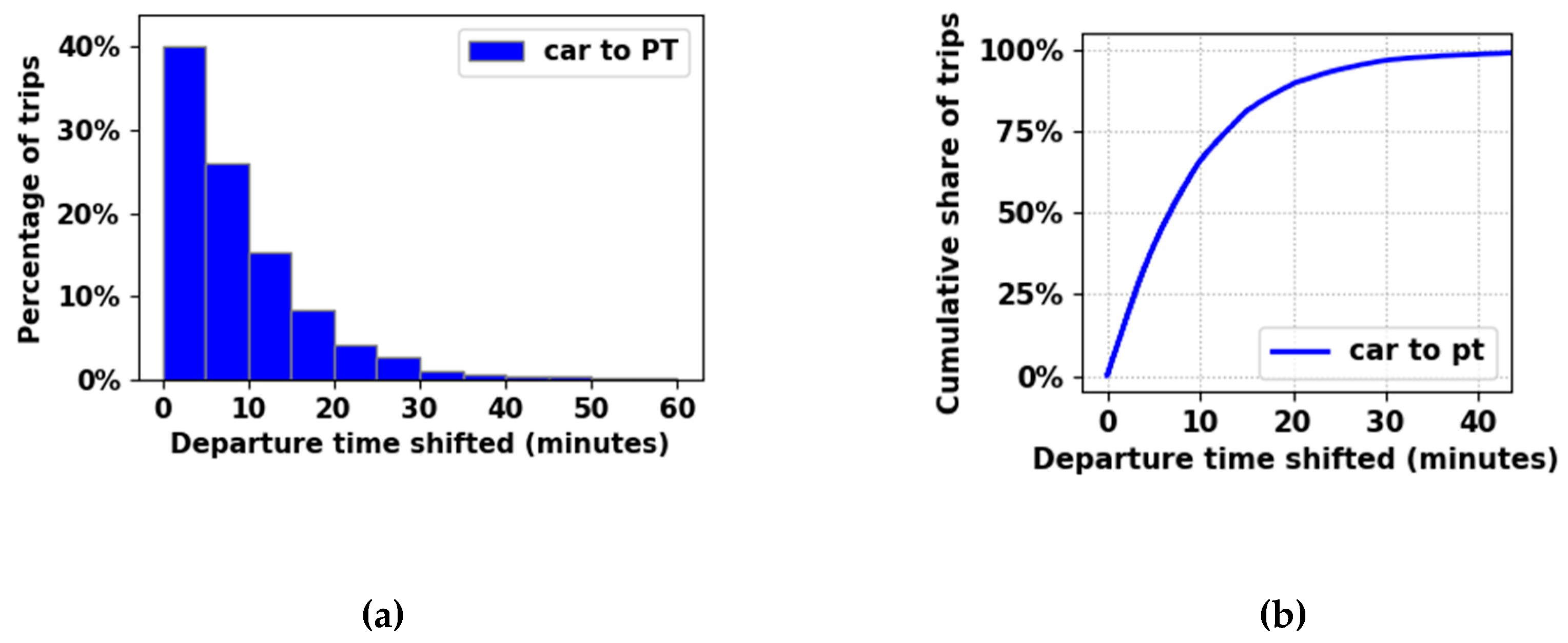
Based on the implemented computation framework, each observed car trip can have different lower-carbon alternatives at the same time, namely, one or several of the following options: walking, biking, or using PT. Around 2% of car trips, mostly shorter than 1 km, have only a walk alternative. Around 58% of car trips have two, and 40% have all the three possible alternatives. Among the 14,500 observed car trips, 14,000 have a lower-carbon alternative with PT and 5900 have a lower-carbon alternative with bike, regardless of travel time changes. Among the PT alternative modes, 67% are bus, 10% metro, 3% city train, 2% tram, and 18% composed of multiple PT modes. Around 63% of PT alternative trips include no transfers, 33% one transfer, 4% two transfers, and less than 1% three transfers. Figure 8 illustrates per-trip travel time changes as a result of modal shift. On average, a PT alternative trip would result in 13 min of increased travel time, and a bike alternative trip would result in 9 min of increased travel time. Figure 9 shows the range and distribution of travel times of observed car trips in comparison to the lower-carbon alternatives. In addition, Figure 10 illustrates per-day travel times represented as total daily travel time (TDT). On average, participants made 1.3 car trips per person-day. Among the 10,000 observed person-days, in 60% (6000) of days, the traveler made a car trip. For these days with car trips, around 2200 person-days include bike alternatives, and around 5700 person-days include PT alternatives, regardless of travel time changes. Figure 10a shows the potential changes in TDT for those days with alternatives. It is seen that in some days, biking or taking PT is almost as fast as driving a car, and therefore the TDT change is closer to zero or even negative. Figure 10b shows the resulting TDTs after potential modal shifts. While the shape of TDT distribution does not change much after modal shifts, the mean and maximum values would increase. Mean observed TDT was 53 min, whereas, mean TDT would be 67 min after modal shifts to PT, and 57 min after modal shifts to biking. When shifting from car to PT, in many cases, the traveler should wait some extra minutes before starting to walk from the origin to the PT stop. Therefore, the departure time is postponed compared to the observed car trip. Figure 11 illustrates such departure time shifts, where it is seen that with 75% of PT alternative trips, the departure time shift would be less than 13 min.

4.2. Potential Travel Time Changes, Emission Reduction, and Physically Active Travel Distance

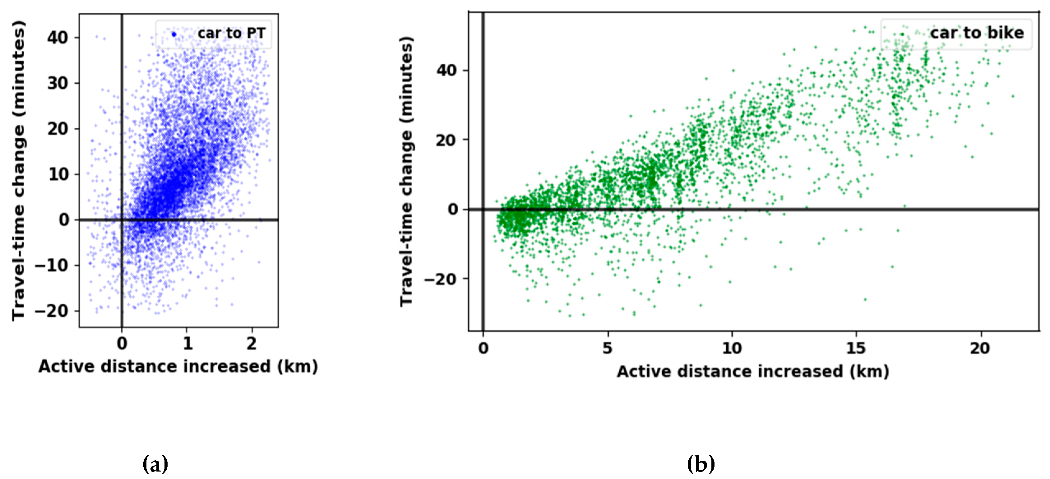
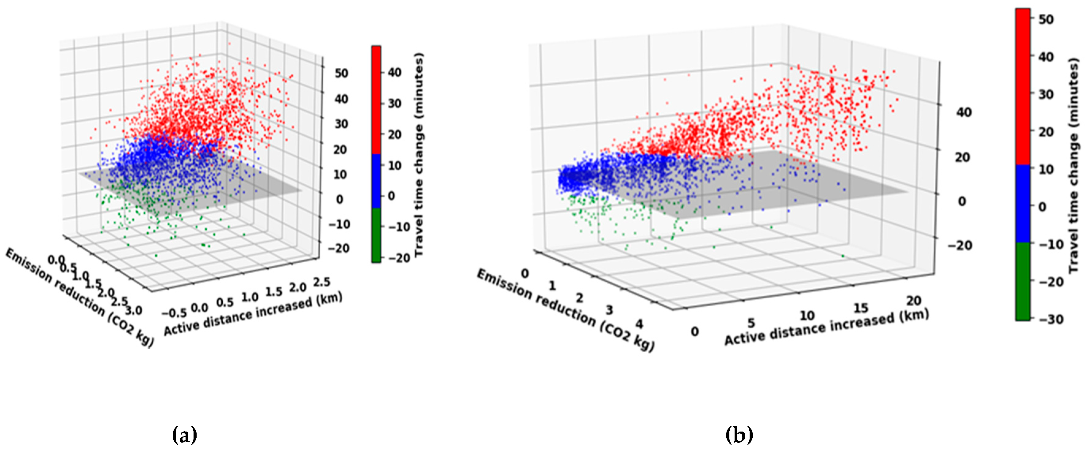
Figure 12 shows changes in travel time versus emission reductions as a result of potential modal shifts. As expected, the general trend of time change (y axis values) increases with larger emission reductions brought by alternatives. The larger observed car emissions imply longer travel distances that would be replaced by a lower-carbon alternative. The figure shows that for some trips, biking or taking PT is as fast as driving a car, and thus the travel time difference is closer to zero. There are also cases where PT or biking is faster than car driving and thus travel time difference is negative. The following Figure 13 provides additional insight on changes in travel time compared to changes in the physically active distance by walking or cycling. As seen in the figure, the changes in the physically active distance when shifting to PT is limited to a maximum of 2.5 km, the reason being that in most PT trips the physically active distance is the access/egress walk to the PT stop, with some cases having walk legs between the intermediate stops. On the other hand, when shifting to biking, the physically active distance increases up to 20 km as the whole trip would be traveled with a bike. Figure 14 depicts all three parameters together, with the gray plane indicating no travel time change. These figures show the extent of possible trade-offs of maintaining the same or even reducing travel time in relation to emissions and physical activity.

4.3. Influence of Travel Time Threshold Variance

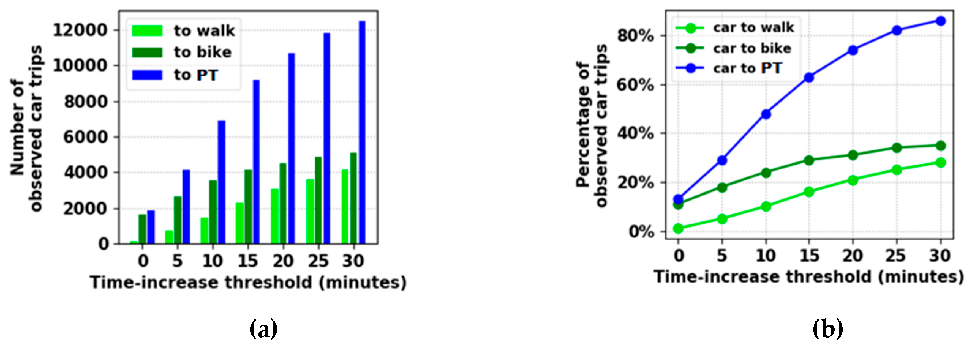
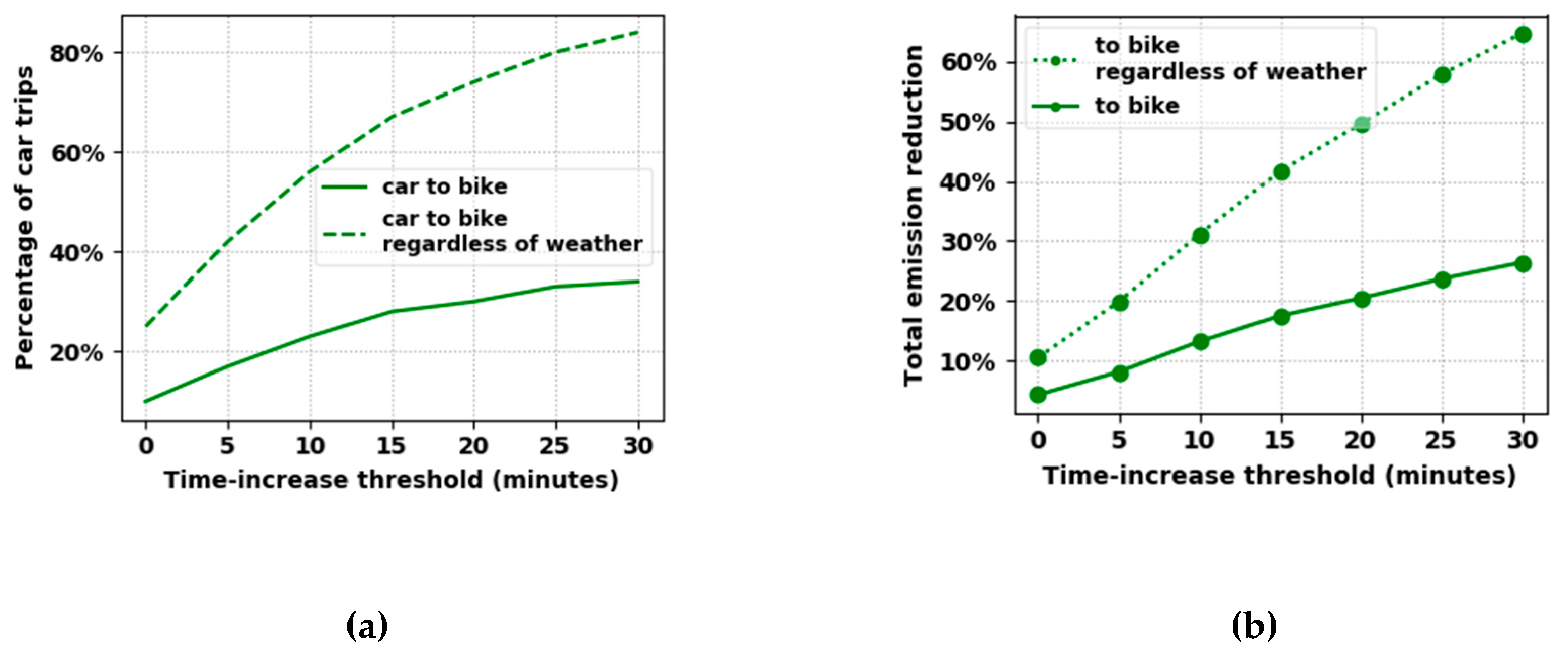
As explained in Section 2, we can classify alternatives as feasible and non-feasible so that a modal shift is deemed acceptable when the increased travel time with the alternative is not more than an assumed threshold. In this section, we consider different values for the time-increase threshold and present the outcomes. As expected, Figure 15a,b show the growing potential of lower-carbon alternatives with longer time-increase thresholds. Figure 15a illustrates the absolute numbers and Figure 15b the percentages of observed car trips that could have a potential lower-carbon alternative depending on the travel time increase threshold.
Figure 16a shows the change in distance that the alternative modes could potentially have depending on the time-increase threshold. Without considering any time threshold, the distance coverages of low-carbon modes would be very similar, and on average around 6 km for any of the walk, bike, and PT mode groups. However, as walking is the slowest of the low-carbon modes, its distance coverage gets limited to a maximum of about 1.5 km after applying the time thresholds. Subsequently, potential emission reduction by walking would be also much smaller than by biking or using PT. Traveling by PT has, on average, the longest distance coverage among the alternative modes. Figure 16b compares the travel distance of alternatives with the observed car trips. It is seen that bike and walk alternatives tend to have a travel distance slightly shorter than the observed car trips, which could be said to help with reducing travel time. Figure 16c compares the trip speed of alternatives with observed car trips. As expected, the smaller time-increase thresholds include mostly the relatively faster alternatives, while the larger thresholds included more of the relatively slow alternatives, including the ones slower than the observed car trip, i.e., speed ratio smaller than 1.0.
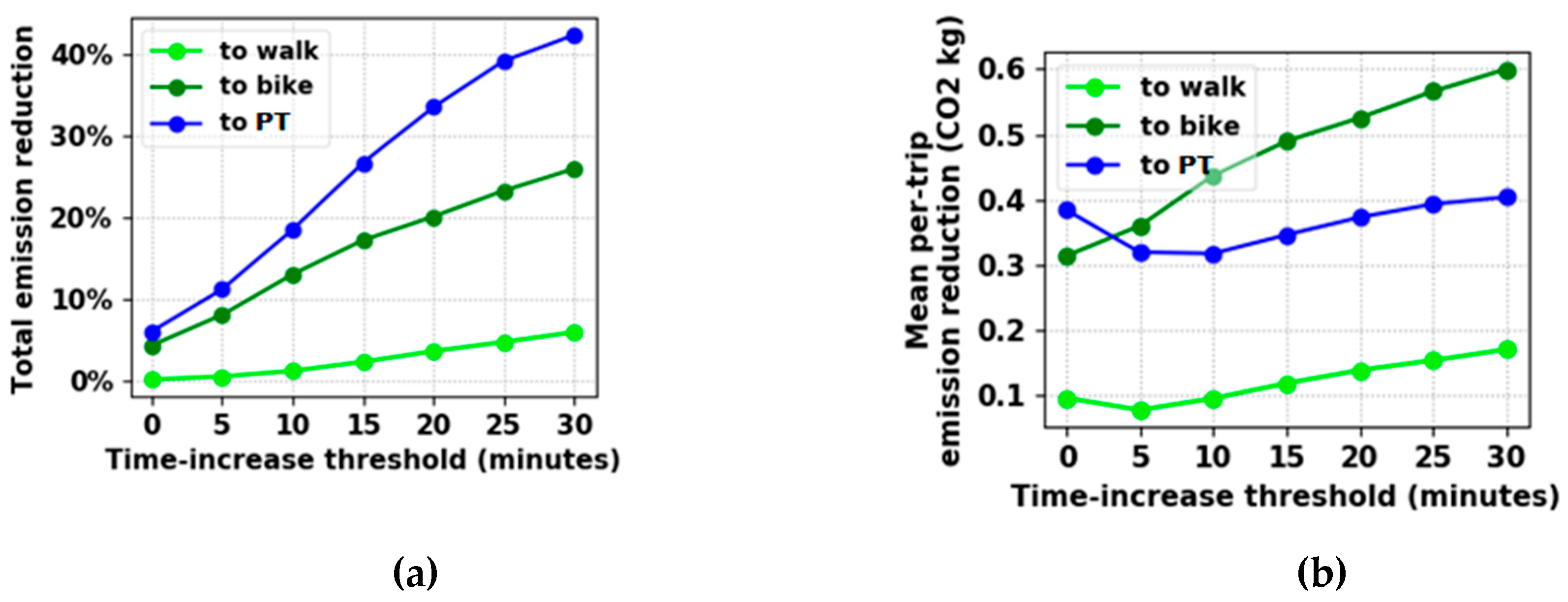
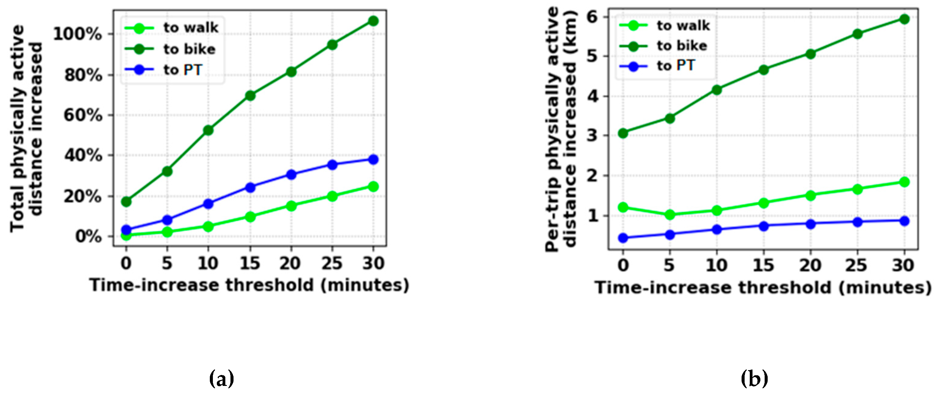
Figure 17a shows the growing potential emission reductions with larger time-increase thresholds. For example, with a maximum of 5 min per-trip time increase, we could get a total 11% carbon emission reduction by shifting from car to PT. In addition to a larger percentage of car trips being substituted with an alternative, the larger emission-reduction percentages also imply more of the longer distance car trips being substituted with an alternative (OD distances shown above in Figure 17a. Figure 17b shows changes in per-trip emission reductions with varying time-increase thresholds, measured as volumes of CO2 kg. Figure 18a shows the total increase of physically active distances with larger time-increase thresholds, while Figure 18b shows the per-trip average changes of physically active distances.
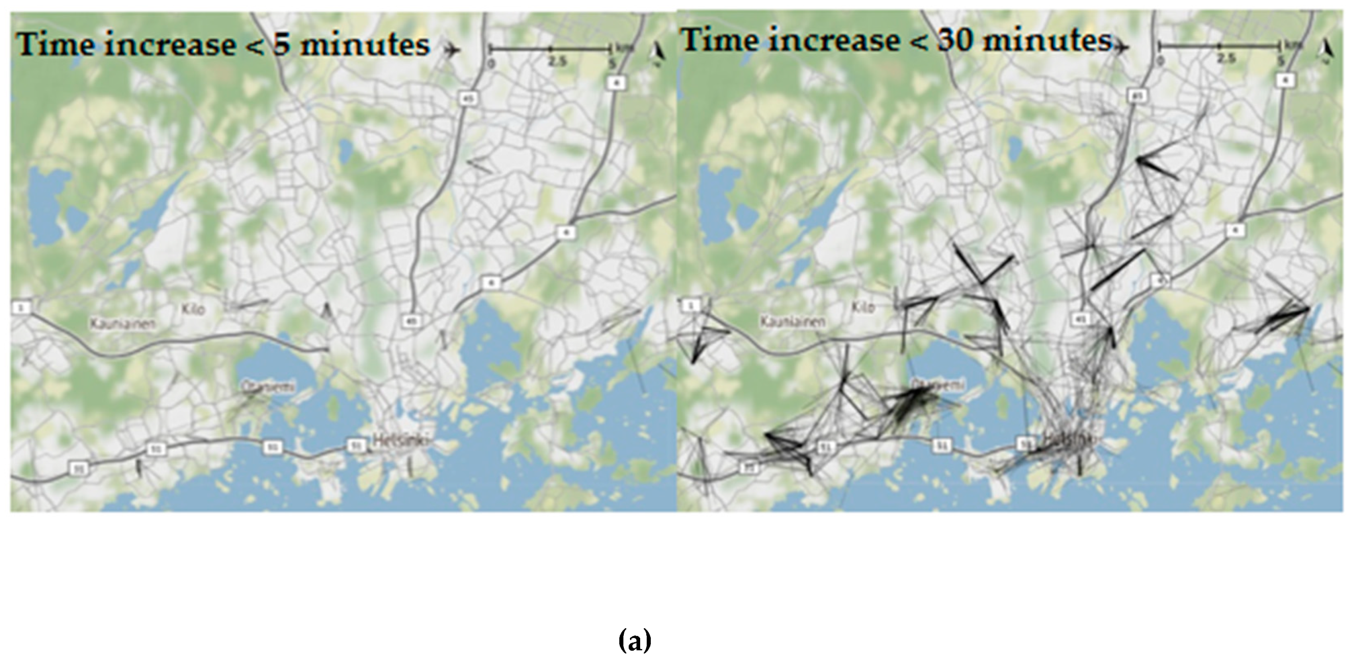
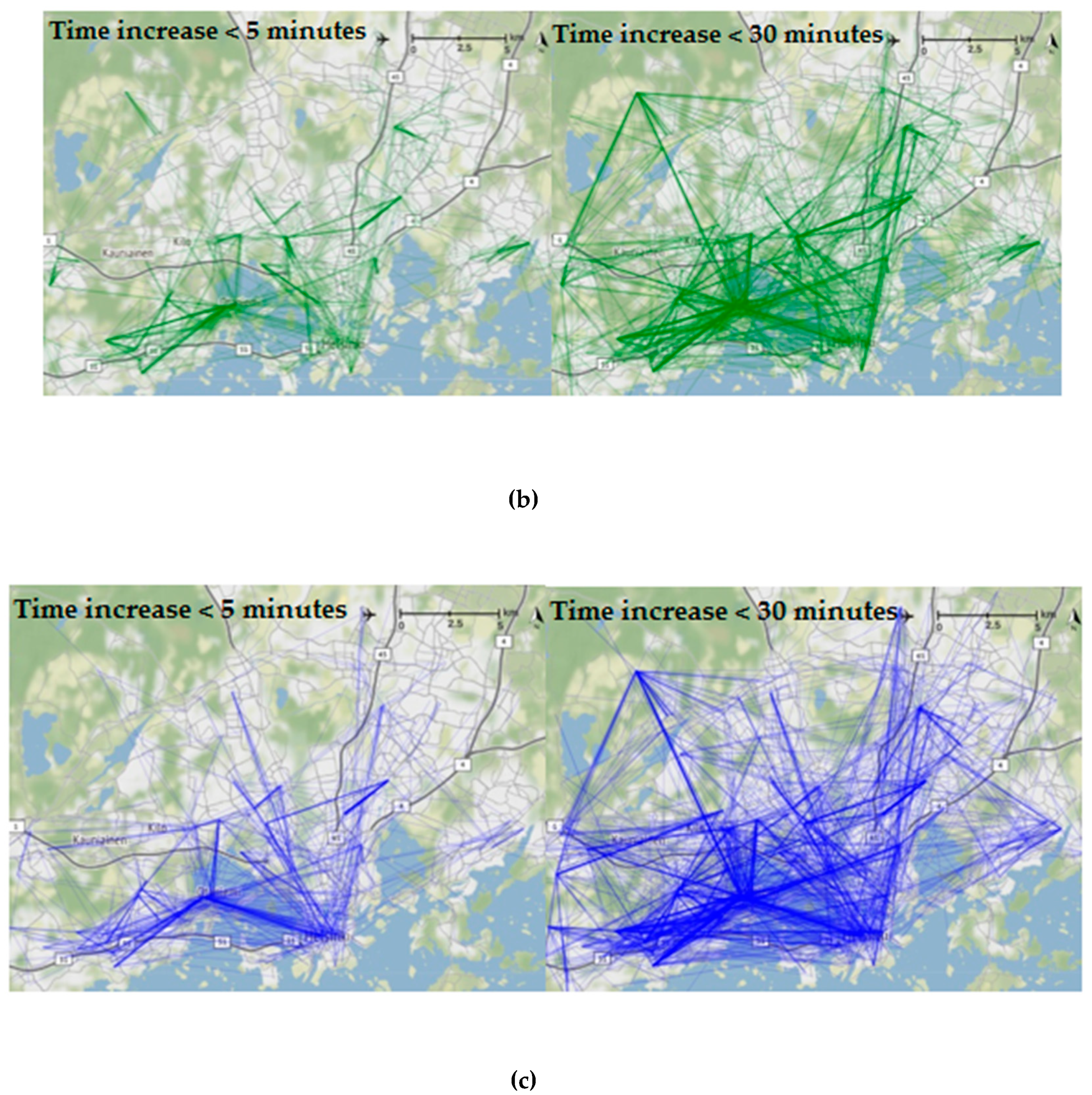
Figure 19 shows total daily travel times depending on time-increase thresholds. The distribution shape of TDTs per person-day and its standard deviation do not change much with the time-increase threshold. The standard deviation is around 30 min across all thresholds. However, with larger thresholds, the range of TDT slightly expands as large as 12 min and the mean TDT increases as large as 5 min. Figure 20 shows the potential alternatives as weighted OD lines, for time-increase thresholds of 5 and 30 min.

4.4. Alternatives in Relation to the Weather Context

Figure 21 shows an overview of potential mode choices per day and share of physically active travel distances in relation to temperature and precipitation. In the case study region of the HMR, on average, 36% of days per year were suitable for biking assuming the temperature and precipitation thresholds outlined in Section 2. Naturally, in other cities, the bike-friendly days and projected bike alternatives will be different depending on the climate. Figure 22 compares the potential changes after modal shift to bike, with and without considering temperature and precipitation.

5. Discussion and Conclusions

This research developed an open-source computational framework prototype for analysis of smartphone-based travel data, with the objective to explore the potential of modal shift to lower-carbon modes while accounting for travel time, emissions, and physical activity. This is a transferable framework that can be used for any target urban region, with the core computation and visualization source-code remaining unchanged. Few changes might be needed in the configuration of algorithms or open-data retrieval channels. For example, the values of emission per passenger-km could be easily edited depending on the region. For computation of alternative trips, if a public web-based OTP server is available for the region (as is the case in Finland), the current link to the OTP server could be replaced. Alternatively, an offline OTP server could be installed that holds PT schedule information of the target region. In this paper, we have evaluated the framework on a case study of the HMR and discussed answers to questions such as potentially acceptable increases in travel time in relation to emissions and physical activity. The following subsections discuss key findings and potential directions for further development.

5.1. Highlights of Case Study Findings on the Potential for Modal Shift

Case study results from the HMR show examples of different components that this computational framework includes. The analysis presented in the previous section is not intended to be representative of the HMR residents and their travel patterns, but to showcase the extent of the proposed computational framework. It should be noted that implications might differ depending on the city where the travel data is collected as well as the extent and diversity of the collected data. The following are summarized examples of how time-increase thresholds affect potential changes in the HMR. For instance, by assuming a maximum 5 min per-trip travel time increase, 30% of car trips could potentially shift to PT, resulting in 11% total carbon emission reduction (mean 0.35 CO2-kg per trip) and 10% increased physically active travel (mean 0.5 km per trip). Likewise, 19% of car trips could potentially shift to cycling, leading to 9% total carbon emission reduction and 36% increased physically active travel. In comparison, the previous study based on a household travel survey in Madrid has shown that 18% of reported car trips have a low-carbon alternative, however by considering only cases with no increase in travel time [18].
On the other hand, in addition to possible travel time increases, other factors such as the number of transfers from one PT line to another could affect mode choices. In the HMR case study, around 63% of PT alternative trips required no transfer, 33% required one transfer, 3% required two transfers, and 1% required three or more transfers. This computational framework can also identify opposite cases, when car trips do not have a feasible PT alternative. From our data sample, around 3% of the 14,500 observed car trips have no feasible PT alternative. The majority (75%) of such trips have a travel distance of less than 1.4 km, with walking or biking as the only possible alternatives from origin to destination. In addition, around 35% of observed car trips without a PT alternative were short trips with travel distances of less than 500 m. Looking further into this case of short trips, around 1800 observed trips had a distance smaller than 500 m, from which, the majority 77% were walk trips, and the rest were car and bike trips. Among those observed 200 short car trips, only 25% have a potential PT alternative. Thus, in addition to estimates on the aggregate level, this computational framework can allow further segmentation of trip properties, in order to obtain a more diverse understanding of existing and potential mode choices.
In contrast to previous developments using smartphone-based data collection, this computational framework accounts for daily weather conditions in relation to choosing to cycle. This information is particularly important due to climate change adaptation, and not just mitigation in terms of GHG emission reduction. In fact, even the HMR has seen changes in weather patterns, especially temperature increase but also changes in precipitation frequency. Thus, this computational framework can cast additional understanding of potential mode change not just in the HMR, but also in other cities, especially if further combined with forecasts of weather pattern changes. On the other hand, personal preferences and physical ability could limit cycling to rather short trips and relatively flat terrain, varying from city to city [75]. With this in mind, the HMR with relatively flat terrain has plenty of latent potential for cycling, but similar conclusions for other regions will have to be evaluated based on specific city conditions. For example, Morency, Verreault, and Frappier [58] conclude that most travelers in Montreal bike up to 5.4 km distance. Although our method now does not constrain cycling travel distance with a maximum value in the formulation of a computational framework, the analysis shows that cumulative distribution of travel distances is such that 75% of the computed bike choices are shorter than 6.5 km, if we consider a maximum 10 min travel time increase. In the HMR case study, the average walk distance involved in observed car trips was 150 m. As seen in Section 4.1, the physically active walk distance would increase up to 2.5 km by modal shift to a PT alternative. However, for around 2% of the observed car trips, the walk distance would actually decrease up to 500 m after shifting to a PT alternative, which is usually unexpected. Looking at these cases shows that such observed car trips had much longer access/egress walk distances of on average 1.5 km. It could be said that walk legs have been long possibly due to parking spots being located far from origin/destination, and that they also relate to longer door-to-door travel distances of such car trips, which is 12 km on average.

5.2. Usefulness of Understanding Modal Shift Potential

The proposed computational framework could be useful in the process of policy and planning decisions across spatial and temporal scales, from macroscopic to microscopic [54]. In particular, numerical estimations and visual representations of ODs, travel time, and mode choice percentages provided are essential for initiating discussions across a range of stakeholders responsible for enabling transition to a sustainable mobility system. In particular, more summative and aggregate values are useful for discussions around regional policies. In addition, looking at values for particular trip characteristics can enlighten decisions about street design or mobility service and behavioral change experiments. Examples of large-scale policy measures are the ongoing discussion about road pricing in the HMR, and the already implemented changes in PT tariff zones, where computing potential for modal shift can play an important role in identifying latent demand for low-carbon and non-priced modes, such as cycling. On a smaller scale, zooming into certain areas to identify potential for modal shift can inform parking pricing and supply choices, or inform prioritization for cycling lane improvements. Having in mind recent developments, such as introducing a bike-sharing scheme that has been also implemented in central parts of the HMR, understanding potential for mode shift can inform decision-making related to expansion strategy and choosing locations for bike-sharing stations. In addition, besides conventional street design measures, identifying potential for cycling can inform other mobility management measures, such as incentives provided by workplaces. For example, a slightly longer commute by bike may also need additional time for taking a shower at arrival, but would also encourage providing shower services at the workplace. Similarly, potential for cycling can inform decisions regarding financial incentives for purchasing e-bikes.
Understanding the potential for modal shift over time also has important implications for other decisions. From our most recent data, we have seen that remote work measures due to the COVID-19 virus have resulted in a decline of 35% of trips since March 2020. Similarly, people might base their decisions for immobility and remote work also on weather conditions. In relation to the aforementioned bike-sharing system in the HMR, understanding temporal variations of potential for modal shift can also inform decisions about annual periods for system operation. Focusing on the daily level, previous studies have shown that the demand for bike-sharing has a strong inverse relationship with long travel distances, precipitation, and harsh temperatures [76]. Similar aspects have been highlighted in our case study. In addition, for a number of people, there may be a big preference difference in biking during daylight hours versus biking in the dark. These aspects are quite easy to investigate by looking at the time points of the biking trips. From the HMR case study, a slight difference can be seen between bike and other modes, after 16:30. Looking at the mode-specific cumulative distribution of departure hours, for example, 75% of observed car trips took place before 18:00, while 75% of the observed bike trips took place before 17:30 (slightly earlier). Even if this difference is small, short daylight duration can play an important role during autumn and winter months. In a future study, it could be interesting to differentiate between daily work commute and other trips, as it may be possible to classify trips between two locations.
These decisions would have to go hand in hand also with the plethora of other survey methods existing in transport agencies, such as travel experience and stated preference questionnaires and focus groups. For example, the combination of this computational framework and those survey methods can inform the range of acceptable travel time increases in certain regions, or identify safety concerns on certain cycling pathways. Moreover, there is potential for further identifying existing user profiles, which could be then connected to future user personas for which changes in policy, infrastructure, and services have to be made. For example, the observed data of the HMR case study shows (e.g., Figure 7) there are the “cycling enthusiasts” who would bike even outside the assumed temperature and precipitation thresholds. These users have bike-days below 5 °C or even in sub-zero temperatures and on heavy rainy days. A study in Beijing shows that bike-sharing facilities attract travelers from diverse socioeconomic backgrounds and, therefore, biking can be targeted towards a wide range of user profiles [76]. However, decisions around supporting low-carbon transport would inevitably have to take into account the variation in travel time, as a potential constraint on the daily schedules. Here, further research is needed on the potential for the combination of PT and biking as a competitive alternative to car-based daily schedules.

5.3. Challenges and Potentials for Data Collection and Public Engagement using Smartphone Apps

Considering data collection privacy challenges and guided by the most recent General Data Protection Regulation by the EU, this research took a safe approach in preserving participants’ privacy. We do not use methods that infer residential and work locations from travel data or get clues about the identity of the individual participants. Considering the attributes of travel data, although conventional data collection methods provide similar information, applying our framework with smartphone-based datasets enables higher resolution in data collection. In addition, longitudinal data collection enables better understanding of potentials for improvements towards sustainable transport systems, as long-term travel behavior analysis is difficult with conventional data collection methods. The special importance of longitudinal data collection is highlighted also in the case of evaluating policies and experiments before and after implementation.
As expected, there are challenges during the recruitment of participants, even if smartphone apps are gaining popularity worldwide. As mentioned in Section 3, 69 out of the 137 participants submitted the optional online questionnaire. The questionnaire results show that participants came from various residential locations throughout the city, and from all income categories. Unfortunately, the gender distribution was skewed, as there were 53 male and 16 female respondents, which could be associated with a negative trend in technology adoption. This research has presented a proof of concept, targeting future wider spread data collection. As the quantity of the collected travel data affects the quality of analysis, our computational framework will provide more precise results if a more varied population participates, resulting in travel data that is spatially more evenly distributed throughout different areas of the city. Such recruitment of participants can be achieved in future experiments by more systematic but also more resource-intensive methods. However, another fruitful pathway for data collection is existing ticketing and service apps for various transport modes, such as PT or bike sharing. Moreover, as public agencies, such as Helsinki Region Transport (HSL), have decades of knowledge regarding travel patterns based on questionnaires, there is potential in comparing these existing data sources during ongoing recruitment efforts, to decide on more customized recruitment methods for certain types or users or urban regions.
In addition to challenges in the initial recruitment, there is also an underlying challenge of participants stopping or even removing the app for data collection. In general, we devised the methodology to minimize the user interaction and rely on passive collection, in order to avoid unnecessary cognitive overload that might cause drop out. The cumulative number of participants throughout the data collection period was 137. However, participation varied over the years, with people joining and dropping out from the experiment. Yearly participation was 22, 96, 53, and 99 participants in 2016, 2017, 2018, and 2019 respectively. Higher joining rates have definitely been observed after recruitment campaigns, while we have also observed drop outs in participants during summer and winter holiday months, similar to previous challenges with conventional questionnaire response rates. A similar decline in the number of participants was observed after March 2020, once the news about COVID-19 pandemic started to become regular.
In addition to the data collection, having smartphone apps also allows for two-way communication by providing notifications and feedback sent to the user [77,78]. The user remains anonymous when only the mobile app channel is used for communication. Compared to traditional travel questionnaires, it can be challenging to find and reach the respondents again. In future research, the framework presented here could be integrated with web-based and app-based persuasive methods that utilize personalized feedback and gamification [77,78]. For example, the computed alternatives, when having almost equal or reduced travel time, can be recommended to travelers in a way that using PT and biking are gradually perceived as better choices not only because of emission reduction or health benefits, but also as competitors to private cars in terms of travel times.

5.4. Accuracy and Noise in Sampling and Computation

Formulation and implementation of this computational framework also come with challenges regarding accuracy and noise in both data collection and computing. As we know from previous literature, locational accuracy of collected data points depends on many factors, such as clear sky, phone model, and position of the phone (e.g., holding in the hand, pocket, or attached to vehicle) [47,48,49,50]. For example, an experiment of cycling along a 2.5 km urban bike track concluded a maximum inaccuracy of 5 m in the majority of cases and 20 m in the worst-case scenarios [43,44]. In our own experiment, we retrieved the accuracy of sampled data points estimated by the Google Fused Location Provider API [64], resulting in the mean accuracy of all sampled data points being 2.72 m, and the mean accuracy per participant’s smartphone being 5 m. To address the noise challenge, the data collection app discards sampled points that have more than 50 m of inaccuracy. In subsequent steps that detect transport modes and start/end of trip legs for motorized public transport such as bus, the app considers a 100 m threshold to match the GPS traces to the expected path of the scheduled public transport vehicle [45]. Discarding trips that have noise errors is one of the necessary trade-offs that come with using this data collection method. Another common challenge in such studies is validation of the collected smartphone data. For our case study, eight designated participants took part in a pilot in the HMR in August 2016. These eight participants, in addition to having the data collection app on their phones, manually wrote down their trips with the best precision possible, logging minute-accurate start/end of each trip leg, names of the origin/destination transport stations, direction of journey, as well as the transport mode. Afterward, the validation was made by comparing the automatically detected trip legs against the manually logged trips [45]. Finally, in future work, machine learning methods could be integrated into the app to facilitate mode detection and increase its accuracy [33].
To compute accurate and realistic alternative trips, we used the multimodal trip planning approach of OTP APIs [67]. OTP is one of the most well-established open-source software platforms for this purpose, that relies on up-to-date road network data from OpenStreetMaps (OSM), and PT network and schedules data provided by cities or transport agencies as General Transit Feed Specification (GTFS) files [79,80]. OTP’s routing API computes trips by using a single time-dependent graph that contains both road and PT network data [81,82]. In particular, OTP computes walk and bike trips using the A-star algorithm with a Euclidean heuristic [83], and computes PT trips, including their walk legs, using the A-star algorithm with the Tung-Chew heuristic [84] for queue ordering. On the other hand, although the computed trip paths and travel distances have very good accuracy, there is a challenge of travel time estimation. For instance, travel times can be longer during the morning and afternoon rush hours as also seen in observed car trips of Figure 9. Currently, our computational framework does not take into account the effect of traffic situations and congestion on the travel times of the low-carbon alternatives. The possible future improvements in travel time estimation are expected to influence the potential of PT alternatives. For example, when computing a bus alternative trip, travel time could be estimated a bit shorter or a bit longer depending on the rush hour as well as whether or not dedicated lanes are available for the particular bus line. Therefore, traveling by bus in rush hour could be sometimes slower, and not necessarily faster. Regarding car travel time variations during the rush hour, we do not need to compute it at the moment, since we take the observed car travel time, as it is. In addition to the existing transport modes used for computation, future development should focus on emerging technologies, such as e-bikes and e-scooters, which could have different implications for travel speed, travel times, and distances.
In this paper, we assumed the carbon footprint of electric public transport (tram, metro, city train) to be zero, as tailpipe emissions. However, this assumption is not accurate if we consider the whole technological lifecycle and source of electricity production. Future development should focus on computing CO2 emissions of electric PT vehicles by knowing the average power consumption (kWh/km) of the vehicle (not the nominal power of the engine) together with the average CO2 production of the electricity (g/kWh). As PT modes can differ from region to region depending on the electricity production and distribution network, further research is needed to obtain those values and use them in the framework for specific regions. In addition, estimating the CO2 emissions per PT traveler is not straightforward. We have used the average occupancy of PT modes in this study. However, on some routes and time points, PT vehicle occupancy can vary a lot. This occupancy is taken into account indirectly through PT schedule frequency, as it is usually designed to accommodate the number of travelers. Moreover, for computing passenger car emissions, we have not taken into account the percentage of non-combustion engine vehicles. Hybrid electric vehicle (HEV), plug-in hybrid electric vehicle (PHEV), and electric vehicle (EV) passenger cars are becoming more widespread in Finland, but due to the lack of data, this would be a future improvement to the data collection, potentially via user input, as well as an improvement for computation of trip parameters.
Another assumption in computation that has been based on the high-quality PT network of the HMR, is the minimum 10 min of idle time used in Section 2 as a threshold to identify trip start/ends, as related to typical waiting times at transfer PT stops. Similar assumptions have been used before [32], but, in some other cities, travelers might wait longer than 10 min for a bus or train. For this reason, future work could test slightly lower or higher threshold values and compare the identified door-to-door trips. Regarding computing cycling paths, other factors, such as wind and vertical geometry could be potential directions for future development. Moreover, computing total travel time of a bike trip could include further developments regarding weather. Further local studies are needed to identify temperature and precipitation thresholds values affecting the decision to cycle (as in Figure 7), as well as to account for additional time spent to get dressed according to weather condition, for example putting on/taking off the weather shielding clothing (i.e., water and windproof jacket, trousers, gloves, and helmet). As the real-time weather condition is now integrated into the framework, future work could also add such extra times for biking for certain temperature or precipitation ranges.

Author Contributions

Methodology, M.B., M.N.M.; software, M.B.; formal analysis, M.B., M.N.M. and J.K.N.; investigation, M.B., I.K.; data curation, M.B., I.K.; writing—original draft preparation, M.B.; writing—review and editing, M.N.M., I.K. and J.K.N.; visualization, M.B.; funding acquisition, M.N.M., I.K. All authors have read and agreed to the published version of the manuscript.

Funding

This research received no external funding.

Acknowledgments

This research was partly funded by the TrafficSense Project as part of the Aalto Energy Efficiency Research Programme, FINEST Twins Center of Excellence, and the Finnish Foundation for Technology Promotion (Tekniikan edistämissäätiö).

Conflicts of Interest

The authors declare no conflict of interest.

Data Availability

A part of the data used to support the findings of this study is available from authors upon request. Shareable data include database schema and data table structures, as well as data records with aggregation level higher than the individual traveler. Full individual trip records and traces cannot be shared due to research terms and GDPR regulations.

References

  1. Banister, D. The sustainable mobility paradigm. Transp. Policy 2008, 15, 73–80. [Google Scholar] [CrossRef]
  2. Cellina, F.; Bucher, D.; Mangili, F.; Simão, J.V.; Rudel, R.; Raubal, M. A large scale, app-based behaviour change experiment persuading sustainable mobility patterns: Methods, results and lessons learnt. Sustainability 2019, 11, 2674. [Google Scholar] [CrossRef] [Green Version]
  3. Shannon, T.; Giles-Corti, B.; Pikora, T.; Bulsara, M.; Shilton, T.; Bull, F. Active commuting in a university setting: Assessing commuting habits and potential for modal change. Transp. Policy 2006, 13, 240–253. [Google Scholar] [CrossRef]
  4. Kim, J.; Choi, K.; Kim, S.; Fujii, S. How to promote sustainable public bike system from a psychological perspective? Int. J. Sustain. Transp. 2017, 11, 272–281. [Google Scholar] [CrossRef]
  5. Mokhtarian, P.L.; Chen, C. TTB or not TTB, that is the question: A review and analysis of the empirical literature on travel time (and money) budgets. Transp. Res. Part A Policy and Prac. 2004, 38, 643–675. [Google Scholar] [CrossRef] [Green Version]
  6. Stopher, P.R.; Ahmed, A.; Liu, W. Travel time budgets: New evidence from multi-year, multi-day data. Transportation 2017, 44, 1069–1082. [Google Scholar] [CrossRef]
  7. Zhang, X.; Guan, H.; Zhu, H.; Zhu, J. Analysis of Travel Mode Choice Behavior Considering the Indifference Threshold. Sustainability 2019, 11, 5495. [Google Scholar] [CrossRef] [Green Version]
  8. Weckström, C.; Kujala, R.; Mladenović, M.N.; Saramäki, J. Assessment of large-scale transitions in public transport networks using open timetable data: Case of Helsinki metro extension. J. Transp. Geogr. 2019, 79. [Google Scholar] [CrossRef]
  9. Haglund, N.; Mladenovic, M.N.; Kujala, R.; Weckstrom, C.; Saramaki, J. Where did Kutsuplus drive us? Ex post evaluation of on-demand micro- transit pilot in the Helsinki capital region. Res. Transp. Bus. Manag. 2019, 32, 100390. [Google Scholar] [CrossRef]
  10. Weckström, C.; MladenoviĆ, M.N.; Ullah, W.; Nelson, J.D.; Givoni, M.; Bussman, S. User perspectives on emerging mobility services: Ex post analysis of Kutsuplus pilot. Res. Transp. Bus. Manag. 2018, 27, 84–97. [Google Scholar] [CrossRef] [Green Version]
  11. Pangbourne, K.; MladenoviĆ, M.N.; Stead, D.; Stead, D. Questioning mobility as a service: Unanticipated implications for society and governance. Transp. Res. Part A Policy Pract. 2019, 131, 35–49. [Google Scholar] [CrossRef]
  12. Glavić, D.; Mladenovic, M.; Luttinen, T.; Cicevic, S.; Trifunovic, A.; Milos, M. Road to price: User perspectives on road pricing in transition country. Transp. Res. Part A Policy Pract. 2017, 105, 79–94. [Google Scholar] [CrossRef]
  13. Gardner, B.; Abraham, C. What drives car use? A grounded theory analysis of commuters’ reasons for driving. Transp. Res. Part F Traffic Psychol. Behav. 2007, 10, 187–200. [Google Scholar] [CrossRef]
  14. Mitra, R.; Ziemba, R.A.; Hess, P.M. Mode substitution effect of urban cycle tracks: Case study of a downtown street in Toronto, Canada. Int. J. Sustain. Transp. 2016, 11, 248–256. [Google Scholar] [CrossRef]
  15. De Witte, A.; Hollevoet, J.; Dobruszkes, F.; Hubert, M.; Macharis, C. Linking modal choice to motility: A comprehensive review. Transp. Res. Part A Policy Pract. 2013, 49, 329–341. [Google Scholar] [CrossRef]
  16. Grotenhuis, J.-W.; Wiegmans, B.W.; Rietveld, P. The desired quality of integrated multimodal travel information in public transport: Customer needs for time and effort savings. Transp. Policy 2007, 14, 27–38. [Google Scholar] [CrossRef]
  17. Monzon, A.; Vega, L.A. How to measure the potential of transferring trips from car to public transport and soft modes—The case of Madrid. In Proceedings of the European Transport Conference, Strasbourg, France, 18–20 September 2006. [Google Scholar]
  18. Monzón, A.; Vega, L.A.; López-Lambas, M.E. Potential to attract drivers out of their cars in dense urban areas. Eur. Transp. Res. Rev. 2011, 3, 129–137. [Google Scholar] [CrossRef] [Green Version]
  19. Beirão, G.; Cabral, J.A.S. Understanding attitudes towards public transport and private car: A qualitative study. Transp. Policy 2007, 14, 478–489. [Google Scholar] [CrossRef]
  20. Sharples, R. Travel competence: Empowering travellers. Transp. Res. Part F Traffic Psychol. Behav. 2017, 44, 63–75. [Google Scholar] [CrossRef]
  21. Van Exel, J.; Rietveld, P. Could you also have made this trip by another mode? An investigation of perceived travel possibilities of car and train travellers on the main travel corridors to the city of Amsterdam, The Netherlands. Transp. Res. Part A Policy Pract. 2009, 43, 374–385. [Google Scholar] [CrossRef]
  22. Stopher, P.R.; Greaves, S.P. Household travel surveys: Where are we going? Transp. Res. Part A Policy Pract. 2007, 41, 367–381. [Google Scholar] [CrossRef]
  23. Bricka, S.; Zmud, J.; Wolf, J.; Freedman, J. Household travel surveys with GPS: An experiment. Transp. Res. Rec. 2009, 2105, 51–56. [Google Scholar] [CrossRef]
  24. Patterson, Z.; Fitzsimmons, K. DataMobile: Smartphone Travel Survey Experiment. Transp. Res. Rec. 2016, 2594, 35–43. [Google Scholar] [CrossRef]
  25. Murakami, E.; Wagner, D. Can using global positioning system (GPS) improve trip reporting? Transp. Res. Part C Emerg. Technol. 1999, 7, 149–165. [Google Scholar] [CrossRef]
  26. Wolf, J.; Oliveira, M.; Thompson, M. Impact of Underreporting on Mileage and Travel Time Estimates: Results from Global Positioning System-Enhanced Household Travel Survey. Transp. Res. Rec. J. Transp. Res. Board 2003, 1854, 189–198. [Google Scholar] [CrossRef]
  27. Clifton, K.J.; Muhs, C. Capturing and Representing Multimodal Trips in Travel Surveys. Transp. Res. Rec. J. Transp. Res. Board 2012, 2285, 74–83. [Google Scholar] [CrossRef]
  28. Wolf, J.; Guensler, R.; Bachman, W. Elimination of the Travel Diary: Experiment to Derive Trip Purpose from Global Positioning System Travel Data. Transp. Res. Rec. J. Transp. Res. Board 2001, 1768, 125–134. [Google Scholar] [CrossRef] [Green Version]
  29. Zhu, L.; Gonder, J.; Lin, L. Prediction of Individual Social-Demographic Role Based on Travel Behavior Variability Using Long-Term GPS Data. J. Adv. Transp. 2017, 2017, 7290248. [Google Scholar] [CrossRef] [Green Version]
  30. Chen, X.; Wan, X.; Ding, F.; Li, Q.; McCarthy, C.; Cheng, Y.; Ran, B. Data-Driven Prediction System of Dynamic People-Flow in Large Urban Network Using Cellular Probe Data. J. Adv. Transp. 2019, 2019, 9401630. [Google Scholar] [CrossRef] [Green Version]
  31. Asakura, Y.; Hato, E. Tracking survey for individual travel behaviour using mobile communication instruments. Transp. Res. Part C Emerg. Technol. 2004, 12, 273–291. [Google Scholar] [CrossRef]
  32. Jiang, S.; Fiore, G.A.; Yang, Y.; Ferreira, J.; Frazzoli, E.; González, M.C. A review of urban computing for mobile phone traces: Current methods, challenges and opportunities. In Proceedings of the 2nd ACM SIGKDD International Workshop on Urban Computing, Chicago, IL, USA, 11 August 2013. [Google Scholar] [CrossRef] [Green Version]
  33. Abdulazim, T.; AbdelGawad, H.; Habib, K.N.; Abdulhai, B. Using Smartphones and Sensor Technologies to Automate Collection of Travel Data. Transp. Res. Rec. 2013, 2383, 44–52. [Google Scholar] [CrossRef] [Green Version]
  34. Lynch, J.; Dumont, J.; Greene, E.; Ehrlich, J. Use of a Smartphone GPS Application for Recurrent Travel Behavior Data Collection. Transp. Res. Rec. 2019, 2673, 89–98. [Google Scholar] [CrossRef]
  35. Cottrill, C.D.; Pereira, F.C.; Zhao, F.; Dias, I.F.; Lim, H.B.; Ben-Akiva, M.E.; Zegras, P.C. Future Mobility Survey: Experience in Developing a Smartphone-Based Travel Survey in Singapore. Transp. Res. Rec. J. Transp. Res. Board 2013, 2354, 59–67. [Google Scholar] [CrossRef] [Green Version]
  36. Vlassenroot, S.; Gillis, D.; Bellens, R.; Gautama, S. The Use of Smartphone Applications in the Collection of Travel Behaviour Data. Int. J. Intell. Transp. Syst. Res. 2015, 13, 17–27. [Google Scholar] [CrossRef]
  37. Prelipcean, A.C.; Gidófalvi, G.; Susilo, Y. MEILI: A travel diary collection, annotation and automation system. Comput. Environ. Urban Syst. 2018, 70, 24–34. [Google Scholar] [CrossRef] [Green Version]
  38. Safi, H.; Assemi, B.; Mesbah, M.; Ferreira, L.; Hickman, M.; Information, R. Design and Implementation of a Smartphone-Based Travel Survey. Transp. Res. Rec. J. Transp. Res. Board 2015, 2526, 99–107. [Google Scholar] [CrossRef]
  39. Nitsche, P.; Widhalm, P.; Breuss, S.; Brändle, N.; Maurer, P. Supporting large-scale travel surveys with smartphones—A practical approach. Transp. Res. Part C Emerg. Technol. 2014, 43, 212–221. [Google Scholar] [CrossRef]
  40. Gadzinski, J. Perspectives of the use of smartphones in travel behaviour studies: Findings from a literature review and a pilot study. Transp. Res. Part C Emerg. Technol. 2018, 88, 74–86. [Google Scholar] [CrossRef]
  41. Wang, Z.; He, S.Y.; Leung, Y. Applying mobile phone data to travel behaviour research: A literature review. Travel Behav. Soc. 2017, 11, 141–155. [Google Scholar] [CrossRef]
  42. Chu, H.; Raman, V.; Shen, J.; Kansal, A.; Bahl, V.; Choudhury, R.R.; Raman, V.; Shen, J.; Kansal, A. I am a smartphone and I know my user is driving. In Proceedings of the 2014 Sixth International Conference on Communication Systems and Networks (COMSNETS), Bangalore, India, 6–10 January 2014; pp. 1–8. [Google Scholar]
  43. Bierlaire, M.; Chen, J.; Newman, J. A probabilistic map matching method for smartphone GPS data. Transp. Res. Part C Emerg. Technol. 2013, 26, 78–98. [Google Scholar] [CrossRef]
  44. Liebner, M.; Klanner, F.; Stiller, C. Active safety for vulnerable road users based on smartphone position data. In Proceedings of the 2013 IEEE Intelligent Vehicles Symposium (IV), Gold Coast, Austrslia, 23–26 June 2013; pp. 256–261. [Google Scholar]
  45. Rinne, M.; Bagheri, M.; Tolvanen, T.; Hollmén, J.; Guidotti, R.; Monreale, A.; Pedreschi, D.; Abiteboul, S. Automatic Recognition of Public Transport Trips from Mobile Device Sensor Data and Transport Infrastructure Information. In Proceedings of the International Workshop on Personal Analytics and Privacy (PAP 2017); Springer International Publishing AG: Cham, Switzerland, 2017; Volume 10708 LNCS, pp. 76–97. [Google Scholar]
  46. Servizi, V.; Pereira, F.C.; Anderson, M.K.; Nielsen, O.A. Mining User Behaviour from Smartphone Data, a Literature Review. arXiv 2019, arXiv:1912.11259. [Google Scholar]
  47. Jiang, S.; Ferreira, J.; González, M.C. Activity-Based Human Mobility Patterns Inferred from Mobile Phone Data: A Case Study of Singapore. IEEE Trans. Big Data 2017, 3, 208–219. [Google Scholar] [CrossRef] [Green Version]
  48. Du, J.; Aultman-Hall, L. Increasing the accuracy of trip rate information from passive multi-day GPS travel datasets: Automatic trip end identification issues. Transp. Res. Part A Policy Pract. 2007, 41, 220–232. [Google Scholar] [CrossRef]
  49. Hemminki, S.; Nurmi, P.; Tarkoma, S. Accelerometer-based transportation mode detection on smartphones. In Proceedings of the 11th ACM Conference on Embedded Networked Sensor Systems—SenSys ’13; ACM Press: New York, NY, USA, 2013; pp. 1–14. [Google Scholar]
  50. Shin, D.; Aliaga, D.; Tuncer, B.; Arisona, S.M.; Kim, S.; Zünd, D.; Schmitt, G. Urban sensing: Using smartphones for transportation mode classification. Comput. Environ. Urban Syst. 2015, 53, 76–86. [Google Scholar] [CrossRef]
  51. Patterson, Z.; Fitzsimmons, K.; Jackson, S.; Mukai, T. Itinerum: The open smartphone travel survey platform. SoftwareX 2019, 10, 100230. [Google Scholar] [CrossRef]
  52. Yazdizadeh, A.; Patterson, Z.; Farooq, B. An automated approach from GPS traces to complete trip information. Int. J. Transp. Sci. Technol. 2019, 8, 82–100. [Google Scholar] [CrossRef]
  53. Shankari, K.; Bouzaghrane, M.A.; Maurer, S.M.; Waddell, P.; Culler, D.E.; Katz, R.H. e-mission: An Open-Source, Smartphone Platform for Collecting Human Travel Data. Transp. Res. Rec. 2018, 2672, 1–12. [Google Scholar] [CrossRef]
  54. Harrison, G.; Grant-Muller, S.M.; Hodgson, F.C. New and emerging data forms in transportation planning and policy: Opportunities and challenges for “Track and Trace” data. Transp. Res. Part C Emerg. Technol. 2020, 10, 2672. [Google Scholar] [CrossRef]
  55. Bagheri, M.; MladenoviĆ, M.N.; Kosonen, I.; Nurminen, J.K.; Roncoli, C.; Ylä-Jääski, A. A Computational Framework for Revealing Competitive Travel Times with Low-Carbon Modes Based on Smartphone Data Collection. J. Adv. Transp. 2020, 2020, 4693750. [Google Scholar] [CrossRef] [Green Version]
  56. Zhao, F.; Pereira, F.C.; Ball, R.; Kim, Y.; Han, Y.; Zegras, C.; Ben-Akiva, M.; Information, R. Exploratory Analysis of a Smartphone-Based Travel Survey in Singapore. Transp. Res. Rec. 2015, 2494, 45–56. [Google Scholar] [CrossRef]
  57. Ye, N.; Gao, L.; Juan, Z.; Ni, A. Are People from Households with Children More Likely to Travel by Car? An Empirical Investigation of Individual Travel Mode Choices in Shanghai, China. Sustainability 2018, 10, 4573. [Google Scholar] [CrossRef] [Green Version]
  58. Morency, C.; Verreault, H.; Frappier, A. Estimating latent cycling and walking trips in Montreal. In Proceedings of the TRB 2017 Annual Meeting, Washington, DC, USA, 8–12 January 2017. [Google Scholar]
  59. Godefroy, F.; Morency, C. Estimating Latent Cycling Trips in Montreal, Canada. Transp. Res. Rec. J. Transp. Res. Board 2012, 2314, 120–128. [Google Scholar] [CrossRef]
  60. Greaves, S.P.; Ellison, A.; Ellison, R.; Rance, D.; Standen, C.; Rissel, C.; Crane, M.; Standen, C. A Web-Based Diary and Companion Smartphone app for Travel/Activity Surveys. Transp. Res. Procedia 2015, 11, 297–310. [Google Scholar] [CrossRef] [Green Version]
  61. Van Soest, D.; Tight, M.R.; Rogers, C.D.F. Exploring the distances people walk to access public transport. Transp. Rev. 2019, 40, 160–182. [Google Scholar] [CrossRef]
  62. Wang, Z.; Xue, M.; Zhao, Y.; Zhang, B. Trade-off between environmental benefits and time costs for public bicycles: An empirical analysis using streaming data in China. Sci. Total. Environ. 2020, 715, 136847. [Google Scholar] [CrossRef]
  63. Faghih-Imani, A.; Anowar, S.; Miller, E.J.; Eluru, N. Hail a cab or ride a bike? A travel time comparison of taxi and bicycle-sharing systems in New York City. Transp. Res. Part A Policy Pract. 2017, 101, 11–21. [Google Scholar] [CrossRef]
  64. Google Fused Location Provider API. Available online: developers.google.com/location-context/fused-location-provider (accessed on 1 February 2020).
  65. Google Activity Recognition API. Available online: developers.google.com/location-context/activity-recognition (accessed on 1 February 2020).
  66. Safi, H.; Assemi, B.; Mesbah, M.; Ferreira, L. Trip detection with smartphone-assisted collection of travel data. Transp. Res. Rec. 2016, 2594, 18–26. [Google Scholar] [CrossRef]
  67. OpenTripPlanner. Available online: www.opentripplanner.org (accessed on 1 February 2020).
  68. Reittiopas (Trip Planner for Finland). Available online: https://www.reittiopas.fi/ (accessed on 1 February 2020).
  69. Digitransit Platform Routing API. Available online: www.digitransit.fi/en/developers/apis/1-routing-api/ (accessed on 1 February 2020).
  70. Tiwary, A.; Colls, J. Air Pollution: Measurement, modelling and mitigation, 3rd ed.; Routledge: New York, NY, USA, 2010; ISBN 0203871960. [Google Scholar]
  71. LIPASTO—Unit Emissions (Database of Transport Emissions in Finland). Available online: lipasto.vtt.fi/yksikkopaastot/indexe.htm (accessed on 1 June 2020).
  72. The Finnish Meteorological Institute’s Open Data. Available online: en.ilmatieteenlaitos.fi/open-data (accessed on 1 June 2020).
  73. Time Use Survey—Time Use (132 Categories) by Sex in 1999–2000 and 2009–2010. Available online: pxnet2.stat.fi/PXWeb/pxweb/en/StatFin/StatFin__eli__akay/statfin_akay_pxt_007.px/ (accessed on 1 June 2020).
  74. Schönfelder, S.; Axhausen, K.W. Urban Rhythms and Travel Behaviour: Spatial and Temporal Phenomena of Daily Travel, 1st ed.; Ashgate Publishing, Ltd.: Burlington, VT, USA, 2010; ISBN 9780754675150. [Google Scholar]
  75. Heinen, E.; van Wee, B.; Maat, K. Commuting by Bicycle: An Overview of the Literature. Transp. Rev. 2010, 30, 59–96. [Google Scholar] [CrossRef]
  76. Campbell, A.A.; Cherry, C.; Ryerson, M.S.; Yang, X. Factors influencing the choice of shared bicycles and shared electric bikes in Beijing. Transp. Res. Part C Emerg. Technol. 2016, 67, 399–414. [Google Scholar] [CrossRef] [Green Version]
  77. Jariyasunant, J.; Abou-Zeid, M.; Carrel, A.; Ekambaram, V.; Gaker, D.; Sengupta, R.; Walker, J.L. Quantified Traveler: Travel Feedback Meets the Cloud to Change Behavior. J. Intell. Transp. Syst. 2014, 19, 109–124. [Google Scholar] [CrossRef]
  78. Sunio, V.; Schmöcker, J.-D. Can we promote sustainable travel behavior through mobile apps? Evaluation and review of evidence. Int. J. Sustain. Transp. 2017, 11, 553–566. [Google Scholar] [CrossRef]
  79. Kujala, R.; Weckström, C.; Darst, R.K.; MladenoviĆ, M.N.; Saramäki, J. A collection of public transport network data sets for 25 cities. Sci. Data 2018, 5, 180089. [Google Scholar] [CrossRef] [PubMed] [Green Version]
  80. Zahabi, S.A.H.; Ajzachi, A.; Patterson, Z. Transit Trip Itinerary Inference with GTFS and Smartphone Data. Transp. Res. Rec. 2017, 2652, 59–69. [Google Scholar] [CrossRef]
  81. OpenTripPlanner Routing Bibliography. Available online: docs.opentripplanner.org/en/latest/Bibliography (accessed on 1 June 2020).
  82. Delling, D.; Wagner, D. Time-Dependent Route Planning. In Proceedings of the Lecture Notes in Computer Science (Including Subseries Lecture Notes in Artificial Intelligence and Lecture Notes in Bioinformatics), San Jose, CA, USA, 13–17 February 2005. [Google Scholar]
  83. Mandow, L.; De La Cruz, J.P. Multiobjective A * search with consistent heuristics. J. ACM 2010, 57, 1–25. [Google Scholar] [CrossRef]
  84. Tung, C.T.; Chew, K.L. A multicriteria Pareto-optimal path algorithm. Eur. J. Oper. Res. 1992, 62, 203–209. [Google Scholar] [CrossRef]
Figure 1. Door-to-door trips observed during the data collection period, by (a) month; (b) day of month; (c) departure hour during the day.
Sustainability 12 05901 g001
Figure 2. Income and age distribution of study participants as well as that of the whole Helsinki region: (a) Income Range, (b) Age Group.
Sustainability 12 05901 g002
Figure 3. (a) Traveled distances of the observed trips and (b) Days recorded per participant.
Sustainability 12 05901 g003
Figure 4. Spatial distribution of the observed trips illustrated by density map of origins/destinations (map copyright of OpenStreetMaps, under ODbL).
Sustainability 12 05901 g004
Figure 5. (a) Distribution of the observed daily TDTs and, (b) Distribution of the number of observed daily trips per person-day.
Sustainability 12 05901 g005
Figure 6. Distribution of days according to temperature and precipitation, comparing days of the year versus observed trip person-days. (a) Average day temperature, (b) Precipitation per day.
Sustainability 12 05901 g006
Figure 7. Observed mode choices per day in relation to (a) temperature, and (b) precipitation.
Sustainability 12 05901 g007
Figure 8. Per-trip changes in travel time after potential shift from the observed car trip (a) to PT, (b) to bike, and (c) to walk.
Sustainability 12 05901 g008
Figure 9. Travel time of alternative trips in comparison to observed car trips, illustrated by (a) Departure hour during the day, and (b) Month of year.
Sustainability 12 05901 g009aSustainability 12 05901 g009b
Figure 10. Potential per-day travel time changes. (a) Potential increase or decrease in TDTs for person-days that have at least one alternative; (b) TDTs after potential modal shifts from car to alternatives.
Sustainability 12 05901 g010
Figure 11. How much the traveler should wait before leaving for the PT stop, compared to the original departure time observed with private car: (a) Distribution of trips depending on the departure time shifted, (b) Cumulative share of trips depending on the departure time shifted.
Sustainability 12 05901 g011
Figure 12. Potential per-trip changes in travel time versus emission reductions, as a result of modal shift from car, (a) to PT, (b) to bike, and (c) to walk.
Sustainability 12 05901 g012
Figure 13. Potential changes in per-trip travel time versus increased physically active distances, as a result of modal shift from car, (a) to PT, and (b) to bike.
Sustainability 12 05901 g013
Figure 14. Potential travel-time changes versus emission reduction and increased physically active travel, as a result of modal shift, (a) from car to PT; (b) from car to bike.
Sustainability 12 05901 g014
Figure 15. Potential low-carbon alternatives depending on time-increase thresholds: (a) number of observed car trips that could have a lower-carbon alternative; (b) percentage of observed car trips.
Sustainability 12 05901 g015
Figure 16. (a) Potential distance coverage of alternatives: mean OD distances of observed car trips that have a potential alternative. (b) and (c) Comparing travel distances and speeds of alternatives versus observed car trips.
Sustainability 12 05901 g016
Figure 17. Potential emission reductions depending on time-increase thresholds: (a) total; (b) averages per trip.
Sustainability 12 05901 g017
Figure 18. Potential increase in physically active distances depending on time-increase thresholds: (a) total; (b) averages per trip.
Sustainability 12 05901 g018
Figure 19. Potential total daily travel times (TDTs) after modal shifts, depending on the time-increase threshold.
Sustainability 12 05901 g019
Figure 20. Potential modal shifts illustrated as weighted OD lines on map (map copyright of OpenStreetMaps, under ODbL). (a) Car to walk; (b) Car to bike; (c) Car to PT.
Sustainability 12 05901 g020aSustainability 12 05901 g020b
Figure 21. Potential mode choices per day after modal shift to bike, in relation to (a) Average daily temperature and (b) Precipitation per day.
Sustainability 12 05901 g021
Figure 22. Comparing the potential changes after modal shift to bike, with and without considering temperature and precipitation. (a) Car trips with potential bike alternative, (b) Potential emission reduction resulting from modal shift to bike.
Sustainability 12 05901 g022
Table 1. Components of the computational framework together with parameters evaluated in case study results.
ComponentParameters
Summative potential changes with lower-carbon alternatives
  • Per-trip travel time changes.
  • Travel time of alternative trips versus observed car trips, by departure hour and month.
  • Changes in total daily travel time (TDT) for person-days with at least one alternative.
  • TDTs after potential modal shifts.
  • Departure time shifted with public transport (PT) compared to the original departure time observed with car.
Potential travel time changes, emission reduction, and physically active travel distance
  • Potential changes in travel time versus emission reductions.
  • Potential changes in travel time versus increased physically active travel distances.
  • Potential changes in travel time versus emission reduction and increased physically active distance.
Influence of travel time threshold variance
  • Potential modal shifts by variable time-increase thresholds.
  • Potential distance coverage of alternatives.
  • Potential emission reductions.
  • Potential increase in physically active distances.
  • Potential TDTs after modal shifts.
  • Potential modal shifts illustrated as weighted origin-destination (OD) lines on map.
Alternatives in relation to the weather context
  • Potential mode choices per day after modal shift to bike, in relation to temperature and precipitation.
  • Comparing the potential changes with and without considering weather context.
Table 2. Example of an observed car trip and computed alternative trips from our dataset.
Observed TripTotal DurationTotal Distance (km)Duration Traveled by Each ModeDistance Traveled by Each Mode (km)
Walk→Car→Walk00:43:4319.9Car: 00:41:03
Walk: 00:02:40
Car: 19.78
Walk: 0.12
Computed Alternative TripTotal DurationTotal Distance (km)Duration Traveled by Each ModeDistance Traveled by Each Mode (km)
Walk→Bus→Walk→Train→Walk00:45:2818.5Bus: 00:11:00
Train: 00:19:00
Walk: 00:15:28
Bus: 2.9
Train: 14.9
Walk: 0.7