Viability of Agroecological Systems under Climatic Uncertainty

Abstract

To cope with ever-increasing demand and ensure food security, agronomic systems have shifted over time from traditional agriculture, based on the organic fertilization of soils, to intensive and specialized farming that use chemical fertilization. This resulted in increased soil productivity in the short term, but caused serious ecological drawbacks over time (degradation of soil quality, pollution of water and air, loss of biodiversity, erosion, etc.), and even reversed the trend of agricultural productivity. In this paper, we propose a viability theory–based model to study the sustainability of an agricultural system subject to climate uncertainty. Our objective is to determine what farming practices and activity sequences restore soil quality to a desired level while ensuring an acceptable level of productivity in the presence of the risk of major climatic disasters. The model is applied to Guadeloupe, an island in the West French Indies. We found that the results are highly sensitive to the direct effect of hurricanes on the soil’s quality, which, in turn, strongly affects the impact of the other parameters and that the export oriented sector is more vulnerable and less resilient to climatic uncertainties than the sector aimed at the local market.

1. Introduction

It is self-evident to state that agricultural land is essential to life and a valuable resource for most, if not all, countries. Still, its importance seems to only be noticed when productivity declines and our food security is at stake. Soil has been poorly protected and overexploited for decades, which has resulted in its deterioration worldwide (see Figure 1).

Modern agriculture and farming are important human-induced factors in this degradation. Whereas traditional practices are based on organic fertilization and diversified crop production, modern agriculture relies on intensive single-crop production and chemical fertilizers, which together progressively degrade soil quality and reduce its productivity by changing its physical, chemical, and biological composition. Indeed, fertilization and low-quality irrigation water alters the soil’s chemical makeup. Further, plowing, tillage, removal of vegetative cover, and overgrazing make soil more vulnerable to wind and water erosion, and intensive and specialized cultivation exhausts some minerals and water from the soil and damages its microfauna (Blanco-Canqui and Lal [1]).

The shift from traditional practices to highly specialized agricultural systems was, in part, a result of population growth, which increased demand. This shift increased soil productivity in the short term, but generated serious ecological drawbacks in the long term (degradation of soil quality, pollution of water and air, loss of biodiversity, erosion, etc.) and even reversed the trend of agricultural productivity. Modern agricultural systems have since fallen in a vicious cycle, where increasing chemical fertilizers are used to compensate for the loss of productivity, causing more damage to the soil and the environment (pollution of water and air) (Trautmann et al. [2], Conway [3]).

Implementing eco-responsible agricultural practices, based on crop rotations and mixed crop-livestock associations that are less harmful for the soil, is one way to achieve resource (soil) sustainability (Altieri [4], Kremen et al. [5]). At a macro level, this transition is a long-term process that must take populations’ food needs and farming profitability into account. Such a transition is particularly needed in island regions, given the importance of agriculture to their economies (Angeon et al. [6]). A survey of farmers in the French West Indies revealed that the population is aware of the problem that farmers are making soil quality central to their concerns, and they are willing to make efforts and even to sacrifice some of their financial benefits to restore the quality of their land (Angeon et al. [7]).

In this paper, we adopt a micro point of view and consider the problem of the long-term sustainable operation of a single farm, from both the physical (soil quality) and economic (farmer’s revenues) perspectives. Our empirical terrain is Guadeloupe, an island that is part of the French West Indies. In this region of the world, the restoration of soil quality depends (as everywhere else) on the soil’s inherent properties, the type of agricultural practice adopted by the farmer and on recurrent climatic events such as hurricanes.

Our research questions are as follows:

• Given some economic and soil quality constraints, and taking into account the possible occurrence of climatic events, what are the viable crop rotations to grow over a predefined planning horizon?
• How sensitive are these solutions with respect to parameter values?
• Which farming systems or sectors are the most vulnerable to climatic uncertainties?

Given our problem statement, we adopt viability theory (Aubin [8]) as our methodological framework. There is now a long tradition of applying this theory to address problems that are related to the exploitation of renewable resources, e.g., fisheries and forests (see Oubraham and Zaccour [9] for a literature review). A few have applied viability theory to farming; see, e.g., Tichit et al. [10], Sabatier et al. [11], Sabatier et al. [12], Mouysset et al. [13], Tichit et al. [14], Baumgärtner and Quaas [15], Martin et al. [16], Sabatier et al. [17], and Durand et al. [18]; most of which have focused on herd and grassland management problems.

To the best of our knowledge, Durand et al. [18] is the only study that looked at a soil-quality management problem. When considering a single plot of agricultural land, the authors proposed a viability theory-based deterministic model, and looked for agricultural strategies and crop rotations that would restore soil quality to an acceptable level while preserving the farm’s economic profitability. In this paper, we extend their model to a stochastic setting to account for the impact of uncertainty from major climatic events, such as hurricanes, on the system’s evolution. During one season of the year, it is almost a certainty that the West Indies region will be affected by climatic events. The uncertainty relates to their force and the damage they will cause. Given this state of affairs, we believe our model adds a level of realism to what was done in Durand et al. [18].

The rest of the paper is organized, as follows: in Section 2, we extend the model in Durand et al. [18] by introducing climatic uncertainty. In Section 3, we define so-called emergency control, that is, what needs to be done after a climatic event. Section 4 is dedicated to the formal definition of all the elements related to climatic events. The solution method is introduced in Section 5, and the empirical application is presented in Section 6. Finally, we briefly conclude in Section 7.

2. A Stochastic Bio-Economic Model

In this section, we extend the model in Durand et al. [18] to take into account the uncertainty related to major climatic events, e.g., cyclones and hurricanes. As in Durand et al. [18], we consider a one-hectare parcel farm managed over time by a single agent. It is a commercial farm whose production is intended for sale. The planning horizon is T and the current time is denoted by $\tau \in \mathcal{T}=\{0,...,T\}$. The state of the farm is described by two variables: (i) the cash flow $\mathcal{W}\in \mathbb{R}$, i.e., a continuous variable characterizing the financial situation; and, (ii) the soil quality of the parcel, which is an agronomic metric. Evaluating the quality of a soil is a complex operation, as it involves a series of physical, chemical, and biological characteristics. Here, we adopt the General Indicator of Soil Quality (GISQ), which has values in the interval $\left[0,1\right]$ and is based on 54 variables measuring these characteristics (Velásquez et al. [19] and Camacho et al. [20]). Let $\mathcal{I}$ be the GISQ value of the parcel, with $\mathcal{I}\in \mathcal{I}=\{0,...,N_{\mathcal{I}}-1\}$, which is, $\mathcal{I}$ can take a finite number of values.

The evolution of the soil quality depends on its current value $\mathcal{I}$ and on the following two control variables: (i) the crop $\sigma$ grown on the parcel, with $\sigma \in \mathsf{\Sigma }=\{{\sigma }_1,...,{\sigma }_{N_{\sigma }}\}$; and, (ii) the agricultural practice $\pi \in \mathsf{\Pi }=\{{\pi }_1,...,{\pi }_{N_{\pi }}\}.$ To illustrate, in the case studies to follow, the set of crops includes either all or some of the following: plantain, export banana, sugar cane, yam (yellow), yam (Grosse Caille), tomato, eggplant, lettuce, carrot, green bean, cabbage, cassava, melon, cucumber, and turban squash. The set of agricultural practices only includes two elements: (i) conventional practice, which is based on modern practices/tools and chemical fertilization; and, (ii) agroecological practice, i.e., traditional practice based on organic fertilization of the soil or other practices for improved management of agroecosystems. Wezel et al. [21] Let the evolution of the soil quality be described by the following function:

$$\begin{array}{ccccc}\varphi & :& \mathcal{I}\times \mathsf{\Sigma }\times \mathsf{\Pi }& \to & \mathcal{I},\\ & & (\mathcal{I},\sigma ,\pi )& \mapsto & \varphi (\mathcal{I},\sigma ,\pi ).\end{array}$$

Denote by $\delta (\sigma ,\pi )$ the duration of the whole agricultural cycle of a crop $\sigma$ using agricultural practice $\pi$. Subsequently, to each pair $\left(\sigma ,\pi \right)$, we can associate production cycles $\psi$, defined as follows:

$$\begin{array}{ccccc}\psi & :& \mathsf{\Sigma }\times \mathsf{\Pi }& \to & \left[0,\delta (\sigma ,\pi )\right],\\ & & (\sigma ,\pi )& \mapsto & \psi (\sigma ,\pi ).\end{array}$$

Moreover, to each crop and practice $\left(\sigma ,\pi \right)$, we associate its first harvest time $f_c\left(\sigma ,\pi \right)$ and the time duration between two successive harvests $p_c\left(\sigma ,\pi \right)$. The duration of the first production cycle is $f_c\left(\sigma ,\pi \right)$, and the following cycles last $p_c\left(\sigma ,\pi \right)$. If a crop has a single harvest, then $f_c\left(\sigma ,\pi \right)=\delta (\sigma ,\pi )$ and $p_c\left(\sigma ,\pi \right)=0$. Additionally, we suppose that the produce is sold right away after it is harvested.

The revenue from each harvest depends on the crop and the agricultural practice, as well as on the soil quality at the beginning of the cycle. Denote by ℓ the revenue function defined by

$$\begin{array}{ccccc}\ell & :& \mathcal{I}\times \mathsf{\Sigma }\times \mathsf{\Pi }& \to & \mathbb{R},\\ & & (\mathcal{I},\sigma ,\pi )& \mapsto & \ell (\mathcal{I},\sigma ,\pi ).\end{array}$$

Denote by $s\in \mathcal{S}=\{1,...,12\}$ the current month. This discrete variable is needed to deal with the seasonality of some crops, which can be planted or sown only at specific times of the year. Let $\mathsf{\Sigma }\left(s\right)\subset \mathsf{\Sigma }$ be the set of all crops that can be planted or sown during season s. In the deterministic model presented in Durand et al. [18], the only event that must be accounted for over time is the beginning/end of a production cycle. If we use n to refer to an event, and $\tau \left(n\right)$ to its timing, then the next event will happen at

$$\tau (n+1)=\tau \left(n\right)+\psi (\sigma \left(n\right),\pi \left(n\right)).$$

(1)

The above equation assumes that once an agricultural cycle starts, it will reach its end. Here, we suppose that a production cycle may be randomly interrupted by a climatic event, which can occur during a specific period of the year, i.e., hurricane season. Consequently, (1) needs to be modified to account for such an event. We introduce the following additional variables:

• $e_1$: the remaining time before the next end/start of a production cycle,
• $e_0$: the remaining time before the next potential hurricane strikes, and
• $ϵ=min\{e_0,e_1\}$: the remaining time before the next change in the system’s state,

Denote by $e=(e_0,e_1,ϵ)$ the vector of events.

Denote by $H\left(t\right)$ the intensity of a climatic event at time t. We suppose that $H\left(t\right)$ takes its values from a finite and discrete set $\mathcal{H}=\{0,1,...,N_h\},$ where 0 represents the absence of a climatic event and $N_h$ is the highest possible intensity. In the case studies, we assume that $\mathcal{H}=\{0,1,2\},$ where 0 corresponds to no hurricane, 1 to a minor hurricane, which is, a hurricane of intensity 1 or 2 on the Saffir-Simpson hurricane wind scale, and 2 to a major hurricane, that is, a hurricane of intensity 3, 4, or 5 on the Saffir-Simpson scale. In line with what is typically observed in the West Indies, which is the area targeted by our case studies, we assume that a climatic event can happen at most once a year during the hurricanes season, starting at $\beta \in \mathcal{S}$ and ending at $\gamma \in \mathcal{S}$. Denote by $\mathcal{P}(s,h)$ the probability that a hurricane of intensity $h\in \mathcal{H}$ happens during season $s\in \mathcal{S}$.

Depending on its intensity, on the type and state of the planted crops, and on the geological characteristics of a parcel, a hurricane happening at step n can interrupt a production cycle and totally or partially destroy the crop growing on that parcel. Let $\theta \left(n\right)\in [0,1]$ be the level of damage, with 0 and 1 corresponding to no damage to crops and total destruction of crops, respectively. We specify $\theta \left(n\right)$, as follows:

$$\theta \left(n\right)=\mathsf{\Theta }(b,\sigma (n),a(n),E),$$

where E is a vector of fixed and known parameters describing the geological characteristics of the soil parcel, e.g., its slope and wind exposure; $a\left(n\right)$ is the age of the crop occupying the parcel at step n; and, b is the intensity of the hurricane it was exposed to.

If a hurricane strikes during a production cycle, then the revenues and the GISQ will be affected. The revenue loss will depend on the age of the crop at the time the hurricane hits and on the level of damage. Let $a\left(n\right)$ be the age of the crop, and b the intensity of the hurricane, respectively. If no hurricane happens during the production cycle, then the parameter b is set equal to zero. The emergency control $v\left(n\right)$ on the parcel at step n will then be defined by

$$v\left(n\right)=(\sigma \left(n\right),\pi \left(n\right),a\left(n\right),b,c)\in \mathsf{\Sigma }\times \mathsf{\Pi }\times [0,{\delta }_{max}]\times \mathcal{H}\times [0,1].$$

where $c\in [0,1]$ is the GISQ of the soil at the beginning of the agronomic cycle of $\sigma$ (when planted or sown). The new parcel’s GISQ value is given by

$$\mathcal{I}(n+1)=\zeta \left(H\left(n\right),\mathcal{I}\left(n\right),v\left(n\right),ϵ\left(n\right),E\right).$$

Further, cleaning and rehabilitation work have to be carried out on the farm before normal agricultural activities resume, which takes time and involves costs. The duration of the rehabilitation work after a hurricane that happened at step n is defined by

$$T\left(v\right(n\left)\right)=f\left(H\right(n),\sigma (n),a(n),\theta (n\left)\right).$$

The earnings generated by the emergency control $v\left(n\right)$ are defined by

$$\mathcal{L}(\mathcal{I},v(n),ϵ(n\left)\right)=g\left(H\right(n),\sigma (n),a(n),\theta (n),ϵ(n\left)\right),$$

that is, it depends on the hurricane intensity $H\left(n\right)$, the crop type $\sigma \left(n\right)$ and age $a\left(n\right)$, the level of damage $\theta \left(n\right)$, and the time elapsed since the last event $ϵ\left(n\right)$.

2.1. Dynamical System

We let the hurricane intensity $H\left(t\right)$ be a state variable, which adds a new event, e.g., a potential hurricane strike, to the only one considered in the deterministic model, which is, the end/start of a production cycle. The state of the farm (cash flow and soil quality) is determined by the vector

$$x=(\mathcal{I},\mathcal{W},H,e,s,\tau ).$$

(2)

We recall that the control variable is

$$v=(u,a,b,c)\in V,$$

where $u=(\sigma ,\pi )\in U=$$\mathsf{\Sigma }\times \mathsf{\Pi }$ is the control applied to the parcel.

To account for crop seasonality, we define by

$$U\left(s\right)\subset U,U\left(s\right)=\mathsf{\Sigma }\left(s\right)\times \mathsf{\Pi },$$

the set of possible controls on the parcel during a particular season s.

The evolution of the farm is then governed by the following discrete-time dynamical system $\mathcal{G}$:

$$\mathcal{G}=\{\begin{array}{}\mathrm{(3a)}& \tau (n+1)=\tau \left(n\right)+ϵ\left(n\right)\mathrm{(3b)}& s(n+1)=\left(s\right(n)+ϵ(n\left)\right)mod 12,\mathrm{(3c)}& H(n+1)=\{\begin{array}{cc}\mathrm{Generated}\mathrm{following}\mathcal{P},\hfill & \mathrm{if}ϵ\left(n\right)=e_0\left(n\right),\hfill \\ 0,\hfill & \mathrm{otherwise},\hfill \end{array}\mathrm{(3d)}& \mathcal{I}(n+1)=\zeta \left(\mathcal{I}\right(n),v(n),ϵ(n),E),\mathrm{(3e)}& v(n+1)\in \{\begin{array}{cc}\left\{\right(\sigma \left(n\right),\pi \left(n\right),a\left(n\right)+ϵ\left(n\right),H(n+1),c\left(n\right)\left)\right\},\hfill & \mathrm{if}ϵ\left(n\right)=e_0\left(n\right),\hfill \\ \left\{\right(\sigma \left(n\right),\pi \left(n\right),a\left(n\right)+ϵ\left(n\right),0,c\left(n\right)\left)\right\}\hfill & \mathrm{if}ϵ\left(n\right)=e_1\left(n\right)\mathrm{and}\theta \left(n\right)<{\theta }_{max}\hfill \\ \mathrm{and}a\left(n\right)<\delta \left(\sigma \right(n),\pi (n\left)\right),\hfill \\ \left\{\right(\sigma ,\pi ,0,0,\mathcal{I}(n+1)\left)\right|(\sigma ,\pi )\in U\left(s\right(n+1\left)\right)\}\hfill & \mathrm{otherwise},\hfill \end{array}\mathrm{(3f)}& \mathcal{W}(n+1)=\mathcal{W}\left(n\right)+\mathcal{L}\left(\mathcal{I}\right(n),v(n),ϵ(n\left)\right),\mathrm{(3g)}& e_0(n+1)=\{\begin{array}{cc}12-\left(s\right(n)-\beta )\hfill & \mathrm{If}H\left(n\right)>0\mathrm{Or}s\left(n\right)=\gamma ,\hfill \\ 1\hfill & \mathrm{If}H\left(n\right)=0\mathrm{And}\beta \le s\left(n\right)<\gamma ,\hfill \\ e_0\left(n\right)-ϵ\left(n\right)\hfill & \mathrm{Otherwise}\hfill \end{array}\mathrm{(3h)}& e_1(n+1)=\{\begin{array}{cc}T\left(v\right(n\left)\right),\hfill & \mathrm{if}ϵ\left(n\right)=e_0\left(n\right),\hfill \\ p_c(\sigma \left(n\right),\pi \left(n\right)),\hfill & \mathrm{if}ϵ\left(n\right)=e_1\left(n\right)\mathrm{and}\theta \left(n\right)<{\theta }_{max}\hfill \\ \mathrm{and}a\left(n\right)<\delta \left(\sigma \right(n),\pi (n\left)\right),\hfill \\ f_c(\sigma (n+1),\pi (n+1))\hfill & \mathrm{otherwise},\hfill \end{array}\mathrm{(3i)}& ϵ(n+1)=\min \left\{e_0\right(n+1),e_1(n+1\left)\right\}\end{array}$$

The initial condition is $x\left(0\right)=\left(\mathcal{I}\right(0),\mathcal{W}(0),H(0),e(0),s(0),\tau (0\left)\right)$, with $\tau \left(0\right)=0$, $s\left(0\right)=1$, $e_0\left(0\right)=\beta -1$, $H\left(0\right)=0$, $e_1\left(0\right)=0$, $ϵ\left(0\right)=\underset{i=\overline{0,1}}{min}{e}_i\left(0\right)$, $\delta \left(0\right)=0$, $\mathcal{I}\left(0\right)$ and $\mathcal{W}\left(0\right)$ are given and $c\left(0\right)=\mathcal{I}\left(0\right)$.

Equation (3i) serves to update the event vector at each step. Equation (3a) sets the clock on time at each step ($n+1$) by advancing it with $ϵ\left(n\right)$ (the time elapsed between steps n and $n+1$). Equation (3b) does the same thing with the season, while taking into account its cyclicity. The other variables are updated according to the type of current event. At any step n, if the remaining time until the next event is equal to the remaining time until the next hurricane strike ( $ϵ\left(n\right)=e_0\left(n\right)$ ), meaning that the event in question (at step $n+1$) is a hurricane, and then the hurricane intensity is generated following the probability distribution $\mathcal{P}$ (see (3c)). The emergency control $\left\{\right(\sigma \left(n\right),\pi \left(n\right),a\left(n\right)+ϵ\left(n\right),H(n+1),c\left(n\right)\left)\right\}$ has to be applied using (3e). The evolution of the GISQ is given in (3d). The remaining time until the next hurricane is set to the hurricane period of next year, since only one hurricane can occur per year (3g). Otherwise, a production cycle ends on the parcel, leading to the modification of the soil quality following (3d). If the production cycle that just ended is not the last one ($a\left(n\right)<\delta \left(\sigma \right(n),\pi (n)$), then the crop and practice remain the same. We merely update the age of the crop and reset the value of the parameter b to 0. We supposed that a crop with multiple production cycles (harvests) entirely recover after one production cycle. The effect of the hurricane is only felt on the harvest following the hurricane (see (3e)), and a new production cycle starts right away, with the remaining time until the next event on the parcel being $p_c(\sigma \left(n\right),\pi \left(n\right))$ (see (3h)). Otherwise, if the whole agricultural cycle ends (interruption by total distruction from the hurricane or the end of the last production cycle of $\sigma \left(n\right)$), then a new crop and agricultural practice $v(n+1)$ has to be chosen from the set $U\left(s\right(n+1\left)\right)$ for this parcel, as expressed in (3e). The new time until the next event on the parcel ($e_1(n+1)$) is equal to the length of the first production cycle of the new crop, which is, $f_c(\sigma (n+1),\pi (n+1));$ see (3h).

Finally, (3f) updates the economic state of the farm by accumulating at each step the earnings generated by the parcel when a production cycle ends and any expenses resulting from a hurricane strike.

2.2. Viability Constraints and Capture Problem

As in Durand et al. [18], we assume that the farmer aims at achieving the following two main objectives:

• Ensuring an acceptable income throughout the whole planning horizon.
• Restoring the quality of the soil to an acceptable level ${\mathcal{I}}^{*}$ by the end of the planning horizon.

The first objective is economic. Clearly, it can take different forms depending on how one defines an “acceptable” income. One practical option is to retain a minimum threshold $W_{min}$, below which cash flow should not fall at any step. Consequently, we have the following admissible set:

$$\mathcal{K}=\{(\mathcal{I},\mathcal{W},H,e,s,\tau )\parallel \tau \le T,\mathcal{W}-W_{min}\ge 0\}.$$

(4)

The second objective is bio-ecological and it can be translated into a target to reach, i.e.,

$$\mathcal{C}=\{(\mathcal{I},\mathcal{W},H,e,s,\tau )\parallel \tau \ge T,\mathcal{I}\ge {\mathcal{I}}^{*}\}.$$

(5)

An alternative to (5) could be to restore the soil quality to at least a certain level $d\%$ of the initial value $\mathcal{I}\left(0\right)$, which is,

$${\mathcal{C}}_d=\{(\mathcal{I},\mathcal{W},H,e,s,\tau )\parallel \tau \ge T,\mathcal{I}\ge min\{\frac{d}{100}\mathcal{I}\left(0\right);1\}\}.$$

(6)

With the uncertainty that is related to climatic events, we end up with a stochastic capture problem, where we look for initial states of system $\mathcal{G}$ defined by (3a)–(3i), for which there exists at least one viable evolution in $\mathcal{K}$ (4) until it reaches the target $\mathcal{C}$ (5), or ${\mathcal{C}}_d$ (6), with a probability exceeding a certain threshold p (the confidence level). This set is called the stochastic capture basin and it is defined as follows:

$$Cap{t}_{\mathcal{G},\mathcal{P}}(\mathcal{K},\mathcal{C})=\{X_0\in \mathcal{K}\parallel \exists x(.)\mathrm{s}.\mathrm{t}.x\left(0\right)=X_0\&\exists t>0\mathrm{s}.\mathrm{t}.\mathcal{P}(x\left(t\right)\in \mathcal{C}\&\forall n\in [0,t],x\left(n\right)\in \mathcal{K})\ge p\}.$$

(7)

3. The Emergency Control

The emergency control $v=(\sigma ,\pi ,a,b,c)$ includes everything that must be done after a climatic event. The duration, cost, and earnings that result from the emergency control depend on the hurricane’s intensity and the damage it caused. In principle, a large variety of cases could occur, but, for tractability, we focus on two of them:

     

Total destruction of the crops. In this case, the climatic event destroys the totality of the crops on the parcel ($\theta \left(n\right)=1$). If this happens, then the farmer has to carry out cleaning and rehabilitation work on the farm, and remove the damaged crops in order to be able to farm the parcel again. We suppose that the cleaning and rehabilitation work directly depends on the hurricane’s intensity. The corresponding time and cost are denoted $t_c\left(H\left(n\right)\right)$ and $c_c\left(H\left(n\right)\right)$, respectively. The time and cost depend on the type of crop occupying the parcel $\sigma \left(n\right)$ and its age $a\left(n\right)$. Denote the time and cost by $t_r(\sigma \left(n\right),a\left(n\right))$ and $c_r(\sigma \left(n\right),a\left(n\right))$, respectively. Consequently, the duration of the emergency control $v=(\sigma ,\pi ,a,b,c)$ is

$$T\left(v\left(n\right)\right)=t_c\left(b\right)+t_r(\sigma \left(n\right),a).$$

The associated earnings correspond to the total financial flow generated during the time elapsed since the last update $\rho \left(I\right(n),v(n),ϵ(n\left)\right)$ minus the total amount incurred for the cleaning and rehabilitating of the parcel ($c_c\left(H\left(n\right)\right)$ and $c_r(\sigma \left(n\right),a\left(n\right))$). The term $\rho \left(I\right(n),v(n),ϵ(n\left)\right)$ includes the fixed costs and the costs for maintenance, labour, etc., and any other nonrecoverable cost. Therefore, we have

$$\mathcal{L}(\mathcal{I},v,ϵ)=\rho (\mathcal{I},v,ϵ)-\left[c_c\left(b\right)+c_r(\sigma ,a)\right].$$

     

Partial degradation of the crops. In this case, the climatic event only destroys a portion of the crops on the parcel ($\theta \left(n\right)<1$). Here, the farmer must decide, based on a given criterion, whether to bring the crop to maturity, or abandon it and start a new agricultural cycle instead. In practice, this decision will depend on the type of crop, its age, and the earnings it will potentially generate. To keep the model parsimonious, we consider a threshold ${\theta }_{max}$ above which degradation is considered to be total and the farmer decides to drop the crop. To be more realistic, one could let the threshold ${\theta }_{max}$ be a function of all other parameters.

If crop degradation caused by the hurricane is sufficiently low ($\theta \left(n\right)<{\theta }_{max}$), then the emergency control must last as long as necessary for the surviving crops to reach maturity and for the cleaning work to be completed. Because these two processes evolve simultaneously, the duration of the emergency control $v=(\sigma ,\pi ,a,b,c)$ is given by

$$T\left(v\left(n\right)\right)=Max\{{\mathbb{1}}_{\{t_c\left(b\right)\ge \delta (\sigma \left(n\right),\pi \left(n\right))-a\left(n\right)\}}{t}_c\left(b\right),e_1\left(n\right)-ϵ\left(n\right)\}.$$

The earnings that are associated with $v=(\sigma ,\pi ,a,b,c)$ correspond to the gain from the surviving crops minus the total cost (cleaning cost, fixed and set-up costs). We suppose that the earnings from a production cycle are inversely proportional to its level of degradation $\theta$. Knowing that a totally healthy production cycle ($\theta =0$) generates earnings

$$\ell (\mathcal{I}\left(n\right),\sigma \left(n\right),\pi \left(n\right))=m(\mathcal{I}\left(n\right),\sigma \left(n\right),\pi \left(n\right))-h_c(\sigma \left(n\right),\pi \left(n\right)),$$

where $m\left(\mathcal{I}\right(n),\sigma (n),\pi (n\left)\right)$ represents the income from selling the harvest and $h_c(\sigma \left(n\right),\pi \left(n\right))$ the harvesting cost, then the earnings from the surviving crop after a hurricane that caused a level $\theta$ of degradation are equal to

$$(1-\theta )m(\mathcal{I}\left(n\right),\sigma \left(n\right),\pi \left(n\right))-h_c(\sigma \left(n\right),\pi \left(n\right)).$$

Consequently, we have the following expression for the earnings from $v=(\sigma ,\pi ,a,b)$:

$$\mathcal{L}(\mathcal{I},v,ϵ)=(1-\theta )\ell (\mathcal{I},\sigma ,\pi )-\theta h_c(\sigma ,\pi )+\rho (\mathcal{I},v,ϵ)-c_c\left(b\right).$$

Subsequently, the general form of the function $T\left(v\right(n\left)\right)$ for $v\left(n\right)=(\sigma ,\pi ,a,b,c)$ is given by

$$T\left(v\left(n\right)\right)=\left\{\begin{array}{cc}{t}_c\left(b\right)+t_r(\sigma \left(n\right),a),\hfill & \mathrm{if}\theta \left(n\right)\ge {\theta }_{max}\hfill \\ Max\{{\mathbb{1}}_{\{t_c\left(b\right)\ge \delta (\sigma \left(n\right),\pi \left(n\right))-a\left(n\right)\}}{t}_c\left(b\right),e_1\left(n\right)-ϵ\left(n\right)\},\hfill & \mathrm{otherwise}\hfill \end{array}\right.$$

(8)

and for $\mathcal{L}(\mathcal{I},v,ϵ)$ by

$$\mathcal{L}(\mathcal{I},v,ϵ)=\left\{\begin{array}{cc}\rho (\mathcal{I},v,ϵ)-\left[c_c\left(b\right)+c_r(\sigma ,a)\right],\hfill & \mathrm{if}\theta \ge {\theta }_{max},\hfill \\ (1-\theta )\ell (\mathcal{I},\sigma ,\pi )-\theta h_c(\sigma ,\pi )+\rho (\mathcal{I},v,ϵ)-c_c\left(b\right),\hfill & \mathrm{otherwise}.\hfill \end{array}\right.$$

(9)

Note that this expression of revenues is also valid for any other control than the emergency control. Indeed, in the absence of a hurricane, $b=0$ so $\theta \left(n\right)=0$ and $c_c\left(b\right)=0$, which leads to $\mathcal{L}(\mathcal{I},v,ϵ)=\ell (\mathcal{I},\sigma ,\pi )+\rho (\mathcal{I},v,ϵ)$, which is the earnings from a normally completed production cycle.

4. The Climatic Events

This section presents all of the relevant information regarding the climatic events and their related uncertainties.

4.1. Types of Climatic Events

A tropical cyclone is a rotating weather system that forms over the ocean when specific water temperature and air humidity conditions arise simultaneously. A significant amount of ocean water then evaporates quickly, causing an atmospheric disturbance. This results in winds revolving around an axis, under the effect of the earth’s rotation, ultimately causing very strong winds, spiral thunderstorms, and heavy rain. When the maximum sustained surface winds of such formations are less than 39 miles per hour (mph), the cyclone is called a tropical depression, and between 39 and 74 mph, it is called a tropical storm. Beyond 74 mph, the event is referred to as a hurricane if it forms over the North Atlantic or Northeast Pacific Ocean, a typhoon if it forms over the Northwest Pacific Ocean, and simply a cyclone if it forms over the South Pacific or Indian Ocean (Source: NOAA website, Wikipedia, and others.)

The intensity of a hurricane is measured by the Saffir–Simpson Hurricane Wind Scale (SSHWS). It has a 1 to 5 categorization based on the hurricane’s intensity at an indicated time (see

Table 1. Saffir–Simpson Hurricane Wind Scale (SSHWS).

Category	Winds	Damage
1	74–95 mph	Minimal
	119–153 Km/h
2	96–110 mph	Moderate
	154–177 Km/h
3	111–129 mph	Intense
Major	178–208 Km/h
4	130–156 mph	Extreme
Major	209–251 Km/h
5	≥157 mph	Catastrophic
Major	≥252 Km/h

Source: https://www.nhc.noaa.gov/aboutsshws.php.) We talk about a major hurricane for events of categories 3 to 5.

4.2. Climatic Uncertainty

As the Caribbean Basin is one of the most hurricane-prone regions in the world, many meteorological studies are available. Surprisingly, however, the French West Indies seem to be an exception, with relatively few studies.

One of the few dedicated studies of this region is Garnier et al. [22]. The authors obtained data from the French archives in France and the islands of Guadeloupe and Martinique to survey all f the hurricanes that hit the French West Indies between 1635 and 2007. They used the data to build a long-term chronology of hurricane severity and damage in this area and to draw some statistical conclusions from these events, in particular yearly probabilities of hurricanes by category, which are of direct interest to our study. We make use of the results of this work because of its geographical relevance and the reliability of its data sources. In addition, the authors only included hurricanes that actually hit the islands of Guadeloupe and Martinique, which makes the results extremely relevant geographically.

Table 2. Yearly probability of a hurricane strike in the French West Indies, by category.

SSHWS Category	Yearly Probability
5	0.02
4	0.05
3	0.08
2	0.12
1	0.16

presents the yearly hurricane probabilities extracted from [22], which will be used in our numerical illustrations.

4.3. Hurricane Effects

The effects of a hurricane on soil and agriculture depend strongly on the type of agriculture and crops, and the soil’s type, relief, etc. Strong winds may affect the physical characteristics of the soil itself. Strong rainfall may induce flooding that can change the chemical composition of the soil and cause landslides in sloped areas. Ocean wind pressure may result in storm surges that can cause severe salt contamination of the soil in costal areas. All of these factors may disturb the microfauna and ultimately change the biological characteristics of the soil ([23]).

There are currently no studies estimating the effect of hurricanes on the GISQ. Therefore, in our numerical applications, we will look at three arbitrary situations: no effect, moderate effect, and significant effect of a hurricane on the GISQ (the precise meaning of these effects is given in Section 6.1.1).

Strong winds can cause significant structural damage to or uproot crops, and flooding may cause certain crops (especially those growing underground) to gorge with water or to rot, and changes to soil composition can compromise the normal growth of the crops. Spencer and Polachek [24] studied the effects of hurricanes on local crop production in Jamaica and found that crops grown above ground suffer greater damage than those grown below ground. In fact, the only below-ground crops that experience a drop of productivity are yams and potatoes. The vast majority of hurricanes that were considered in this study were minor (category 1 and 2) and their effects on crops are displayed in the first row of

Table 3. Damage caused by hurricanes to crops. (Based on [24] for damages and on [22] for the probabilities).

Climatic Event	Yearly Probability	Above Ground	Below Ground	Water Damaged
Minor	0.28	9.2 %	0%	60.6%
Categories 1–2
Major	0.15	100 %	100%	100%
Categories 3–5

.

We consider, not unrealistically, that the losses are total after a major hurricane strike. Accordingly, our choice to consider a degradation of more than 60% (${\theta }_{max}=0.6$) as a total loss will have no impact on the results as studies indicate that hurricanes of category 3 or more cause at least an 80% loss of production.

Table 3 displays the percentage loss in productivity caused by certain types of climatic events on three categories of crops: the above-ground category, which includes all the crops growing above ground; the water-damaged category, which includes above-ground crops that are vulnerable to flooding; and the below-ground category, which includes crops growing underground that are flood resistant.

5. Solution Method

To compute the stochastic capture basin defined in (7), we adopt a dynamic programming approach. We exploit the following property established in Proposition 1 and Corollary 1: if it is possible (not possible) to reach the target with a certain initial treasury, then it is possible (not possible) to reach it with a higher (lower) treasury.

The stochastic capture basin defined in Equation (7) is the set of initial states

$$X_0=(\mathcal{I}\left(0\right),\mathcal{W}\left(0\right),H\left(0\right),e\left(0\right),s\left(0\right),\tau \left(0\right)),$$

satisfying the constraints stated in (7), which is, there exists an evolution starting from $X_0$ that remains in the set $\mathcal{K}$ during the entire planning horizon and reaches the target $\mathcal{C}$ at the end of that time horizon with a probability greater than or equal to the confidence level.

As $\tau \left(0\right)=0$, $s\left(0\right)=1$, $H\left(0\right)=0$, and $e\left(0\right)=0$ are given data, we can characterize any initial state $X_0$ only by its $\mathcal{I}\left(0\right)$ and $\mathcal{W}\left(0\right)$ values, and write

$$X_0=(\mathcal{I}\left(0\right),\mathcal{W}\left(0\right)).$$

Proposition 1.

Let $(\mathcal{I},\mathcal{W})$ be an initial state from the stochastic capture basin $Cap{t}_{\mathcal{G},\mathcal{P}}(\mathcal{K},\mathcal{C})$; then any initial state $(\mathcal{I},{\mathcal{W}}^{\prime })$ with ${\mathcal{W}}^{\prime }\ge \mathcal{W}$ belongs to $Cap{t}_{\mathcal{G},\mathcal{P}}(\mathcal{K},\mathcal{C})$.

$$(\mathcal{I},\mathcal{W})\in Cap{t}_{\mathcal{G},\mathcal{P}}(\mathcal{K},\mathcal{C})\Rightarrow (\mathcal{I},{\mathcal{W}}^{\prime })\in Cap{t}_{\mathcal{G},\mathcal{P}}(\mathcal{K},\mathcal{C})\forall {\mathcal{W}}^{\prime }\ge \mathcal{W}.$$

Proof. 

Let $B(x,I,p)$ be the minimum budget needed for the evolution $x(.)$ to be viable:

$$B(x,\mathcal{I},p)=min\{\mathcal{W}\parallel x(0)=(\mathcal{I},\mathcal{W})\&\exists t>0\mathrm{s}.\mathrm{t}.\mathcal{P}(x\left(t\right)\in \mathcal{C}\&\forall n\in [0,t],x\left(n\right)\in \mathcal{K})\ge p\}$$

We have,

$$(\mathcal{I},\mathcal{W})\in Cap{t}_{\mathcal{G},\mathcal{P}}(\mathcal{K},\mathcal{C})\iff \exists x(.)\mathrm{s}.\mathrm{t}.B(x,\mathcal{I},p)\le \mathcal{W}.$$

Therefore,

$$\forall {\mathcal{W}}^{\prime }\ge \mathcal{W},B(x,\mathcal{I},p)\le {\mathcal{W}}^{\prime },$$

and consequently

$$(\mathcal{I},{\mathcal{W}}^{\prime })\in Cap{t}_{\mathcal{G},\mathcal{P}}(\mathcal{K},\mathcal{C}).$$

 □

Corollary 1.

If it is not possible to reach the target from an initial state $(\mathcal{I},\mathcal{W}),$ then it is not possible to reach it with less initial treasury.

$$(\mathcal{I},\mathcal{W})\notin Cap{t}_{\mathcal{G},\mathcal{P}}(\mathcal{K},\mathcal{C})\Rightarrow (\mathcal{I},{\mathcal{W}}^{\prime })\notin Cap{t}_{\mathcal{G},\mathcal{P}}(\mathcal{K},\mathcal{C})\forall {\mathcal{W}}^{\prime }\le \mathcal{W}$$

The results presented in Proposition 1 and Corollary 1 imply that, in order to completely characterize the capture basin, it is sufficient to identify its border or, in other words, to find for each initial GISQ the minimum initial treasury ${\mathcal{W}}_{inf}(\mathcal{I},p)$ needed for the restoration, i.e.,

$${\mathcal{W}}_{inf}(\mathcal{I},p)=\underset{(\mathcal{I},\mathcal{W})\in Cap{t}_{\mathcal{G},\mathcal{P}}(\mathcal{K},\mathcal{C})}{inf}\mathcal{W}=\underset{x}{min}B(x,\mathcal{I},p).$$

Therefore, the problem amounts to finding a viable evolution of the system $x(·)$ with the minimum possible restoration budget $B(x,\mathcal{I},p).$ This problem can be formulated as a stochastic shortest-path problem, whose objective is to minimize the expected restoration budget, and which can be solved by dynamic programming.

A feedback solution takes the form of a decision tree that gives a control to apply for each state of the system from where it is possible to reach the target. Knowing that each sequence of controls applied in the past, combined with the realization of the uncertainties (the climatic events that occurred) during that period, leads the system to a specific state, the feedback solution gives a sequence of controls to apply during the next periods. Each branch of the decision tree representing the solution describes the evolution of the system for one possible realization of the uncertainties during the exploitation period.

6. Numerical Results

In this section, we consider some farming systems, to which we will refer as cases in a single-parcel setting.

Table 4. Description of the different cases.

Case	Crops
Case 1	Plantain, Export banana
Banana
Case 2	Plantain, Export banana, Sugar cane
Banana & sugar cane
Case 3	Yam(Yellow), Yam(Grosse Caille), Tomato
Tomato and yam
Case 4	Yam (Yellow), Yam(Grosse Caille), Tomato, Eggplant, Lettuce, Carrot, Green bean, Cabbage, Cassava, Melon, Cucumber, Turban squash
Multicrop
Case 5	Plantain, Export banana, Sugar cane, Yam (Yellow), Yam(Grosse Caille), Tomato, Eggplant, Lettuce, Carrot, Green bean, Cabbage, Cassava, Melon, Cucumber, Turban squash
All crops

lists the crops considered in these cases. Each crop can be used either with a conventional or agroecological practice. Additionally, farmers can choose to leave their land fallow. When coupled with the agroecological practice (short fallow and long fallow), the land is left in simple fallow. When coupled with the conventional practice (improved short fallow and improved long fallow), the fallow is improved with the use of chemical additives or fertilizers.

Each one of the cases listed above represents a type of farming system practiced in the French West Indies: the export sector, specialized in banana and sugar cane (cases C1 and C2); the local market sector, based on diversified vegetable farming (C3 and C4); and, a theoretical case (C5) that combines all of the crops.

Computations were made for various hurricane impacts on the GISQ, initial GISQ levels, time horizons, confidence levels, and fixed costs in order to be able to analyze the effect of each parameter. We always require that the farm remain self-sufficient on average, i.e., we set the economic constraint to 0 ($W_{min}=0$) and impose that the retained solution(s) allow for a positive mean treasury.

All of the case studies concern the Guadeloupe archipelago. For the common elements, we use the same data and parameter values, as in Durand et al. [18]. The other required data and parameter values are estimated in Section 4 and/or displayed in Appendix B and Appendix C.

The rest of the section is divided into two parts. In the first part (Section 6.1), we focus on the capture basins. In particular, we analyze the impact of hurricanes on the GISQ (in Section 6.1.1), the impact of the time horizon (in Section 6.1.2), the impact of crop diversification (in Section 6.1.3), the impact of fixed charges (in Section 6.1.4), and the impact of the initial GISQ (in Section 6.1.5).

In the second part (Section 6.2), we look at viable evolutions. More specifically, we discuss the main characteristics of such evolutions and how they are affected by such features as direct hurricane impact, time horizon, fixed charges, and GISQ improvement level.

6.1. Analysis of Capture Basins

Denote by $Cap{t}_{C_i,T}(I^{*},p)$ the capture basin of Case i for a time horizon T, where the GISQ target is $I^{*}$ with a confidence level p. Concretely, the capture basin is the set of all couples of initial GISQ $I_0$ and budget (initial treasury) that make it possible to reach the target while respecting the imposed constraints.

Each panel in Figure 2 represents a superposition of capture basins of the same case for different confidence levels. For example, in the upper left panel of Figure 2, the surface in represents the capture basin $Cap{t}_{C_1,40}(0.8,0.9),$ whereas represents the capture basin $Cap{t}_{C_1,40}(0.8,0.2)$.

In all cases, as expected, the capture basins get smaller when the confidence level is increased, which is,

$$Cap{t}_{C_i,T}(I^{*},p_1)\subseteq Cap{t}_{C_i,T}(I^{*},p_2),\forall p_1\ge p_2.$$

Indeed, if it is possible to reach the target starting from a certain GISQ and using a certain budget with a confidence level $p_1,$ then it is possible to reach it with a confidence level $p_2\le p_1$.

The higher is the initial GISQ $I_0$, the lower is the minimum budget needed to reach the target. However, the budget is always strictly positive, even when the initial GISQ $I_0$ is larger than the target $I^{*}$, due to the fixed costs and the money needed for planting the first crop. In fact, even if nothing is done (i.e., leaving the parcel in free fallow), the farmer needs to cover the fixed cost that must be paid, regardless of activity.

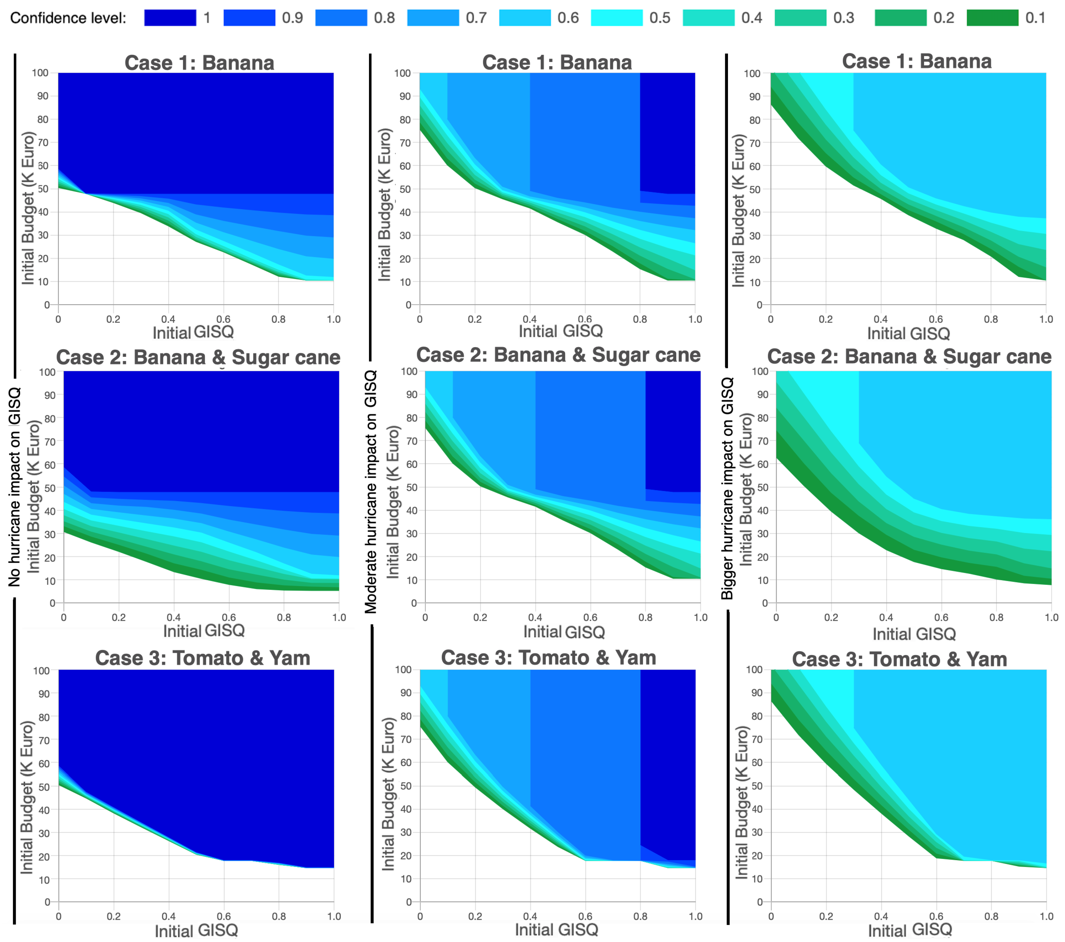
6.1.1. Direct Effect of Hurricanes on the GISQ

The GISQ is a quite recent index describing the soil quality and, thus, there are no studies establishing how its value is affected by hurricanes. To work around this lack of information, our numerical simulations retained the following three arbitrary contexts:

1—No effect: 

regardless of its intensity, a hurricane’s impact on the GISQ is set equal to 0.

2—Moderate effect: 

a minor hurricane decreases the GISQ value by $0.01$, while a major hurricane reduces the GISQ by $0.02$. This case is considered to be the default one, which is, when the effect is not specified in a figure or in the discussion, then it is a moderate effect.

3–Large effect: 

as above, a minor hurricane decreases the GISQ by $0.01$, but a major hurricane reduces the GISQ by $0.05.$

Figure 3 displays the capture basins for a series of cases, where the time horizon is 40 years and the GISQ target $I^{*}=0.8$ for the three different hurricane effects introduced above. A first observation is that when a hurricane has no direct impact on the GISQ (see the first column of Figure 3), then it is always possible to reach the desired level of soil restoration with probability 1, provided that the time horizon is long enough (see Section 6.1.2 ) and a budget is available. Note that the confidence level only affects the minimum budget needed for restoration, due to the assumption that the climatic event does not deteriorate the GISQ.

Now, if a hurricane affects the GISQ, then we notice that the greater the impact, the more difficult it is to restore the soil to the desired level. In particular, for some realizations of the uncertain event, the cost of restoring the soil to the desired level is high, and restoration itself may become infeasible for certain confidence levels. To illustrate, for all displayed cases in Figure 3, it is possible to restore the soil with an initial GISQ of $0.2$, with a confidence level of $0.6$, when we suppose that the hurricane have no direct impact on the GISQ. Restoration is also possible when we assume a moderate effect, but it would take a higher minimum budget. However, restoration is no longer possible if the hurricane has a large impact on the GISQ.

Finally, we note that the capture basin for a large hurricane impact on the GISQ is included in the capture basin with a moderate effect, which is, in turn, included in the no-effect capture basin.

6.1.2. Impact of the Time Horizon

Figure 4 and Figure 5 display the capture basins for cases with different planning horizons (40, 20, 10, and five years) and levels of hurricane impact on the GISQ.

A first takeaway from these figures is that the capture basins shrink and slide to the right as the time horizon gets shorter in all cases, regardless of the level of hurricane impact on the GISQ. This indicates that the less time we have, the more difficult it is to restore the poorest soils, which is quite intuitive. For example, it is possible to bring a soil with a GISQ of $0.2$ to a GISQ of $0.8$ in 40 or 20 years, but not if we only have 10 or 5 years.

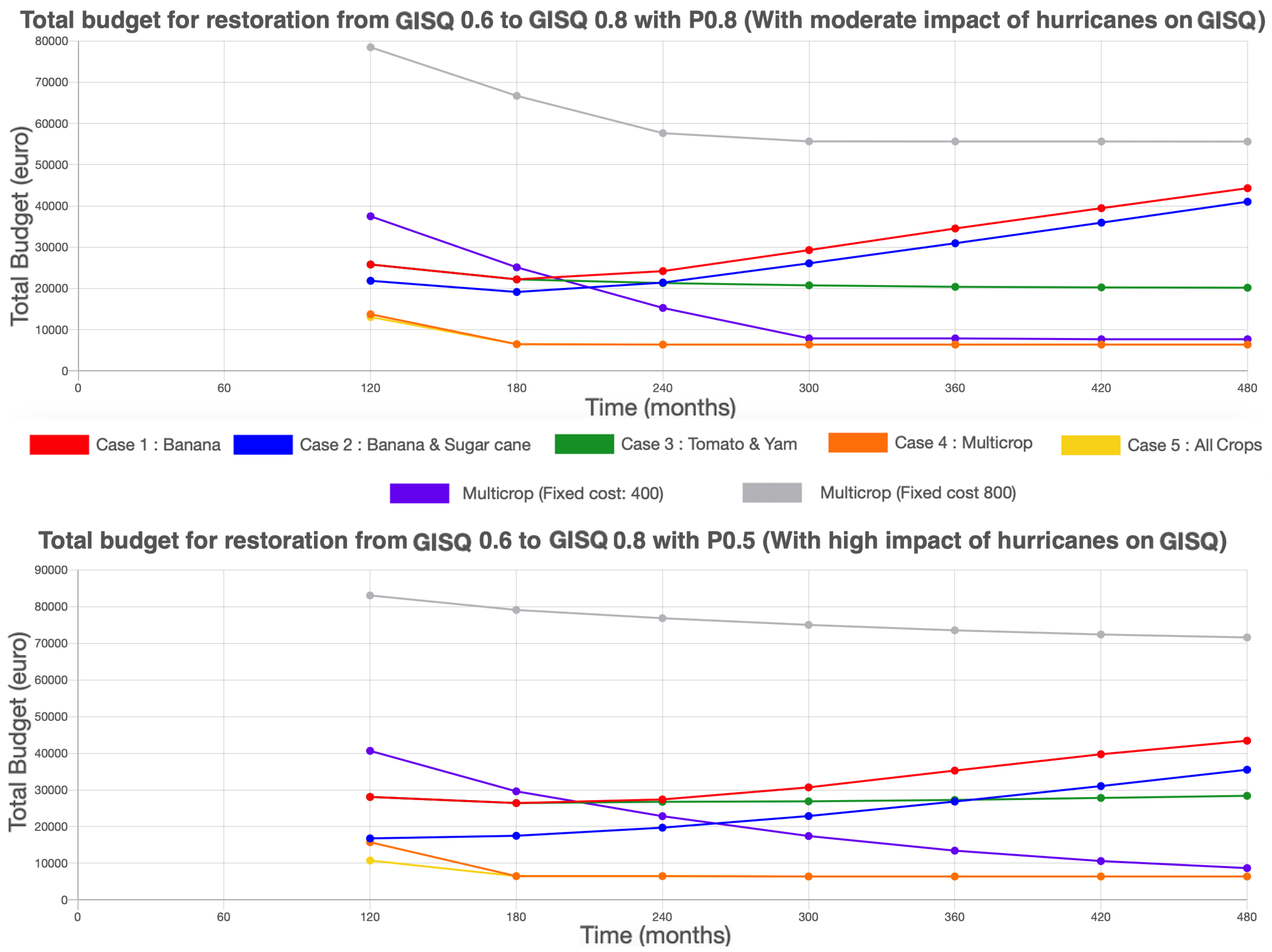
When the improvement is feasible, the minimum restoration budget, for different time horizons, varies across scenarios. To better visualize this behavior, we display in Figure 6, a sample of the total restoration costs as a function of the time horizon for a soil restoration from GISQ $0.6$ to GISQ $0.8$ in the case of a moderate hurricane effect on the GISQ with a probability of $0.8$ (upper part) and in the case of a bigger hurricane impact on the GISQ with a probability of $0.5$ (lower part).

As we would expect, for the same conditions (same initial GISQ and same confidence level), the total restoration budget decreases with the time horizon; see case C4 and its variants (with fixed cost 400 and 800) as well as C3 and C5. Indeed, the less lime is available to restore the soil, the quicker and more efficient the work must be, and the higher is the cost. Moreover, there is a threshold time horizon above which the minimum budget stabilizes and becomes constant. In particular, this happens when the farm is profitable enough: when it just needs a certain amount to start the first production cycle and then it becomes self-sufficient. The time horizon at which the minimum budget stabilizes is the minimum time it takes for farming to become totally self-sufficient.

The minimum time horizon for self-sufficiency depends on the farm’s efficiency level. That is, when the farm faces fewer charges and/or achieves higher incomes, then the timespan for reaching self-sufficiency is shorter. For example, the minimum budget in C4 with a fixed cost of 100 stabilizes before those with fixed costs of 400 and 800. However, for other cases, e.g., C1 and C2, we observe the opposite, which is, globally, the longer the planning horizon, the more expensive it becomes to restore the soil, which seems to be pretty counterintuitive. In fact, this happens when the farm is not profitable enough, i.e., it does not generate sufficient cash to cover all of the operational expenses. Therefore, tautologically, the longer is the time horizon, the higher are the costs to be covered; as a result, the minimum restoration budget increases. This is confirmed by the treasury evolution in the different cases. In those cases with a decreasing restoration budget over time (the profitable cases), the treasury trend is increasing and ends up with a surplus. On the other hand, the cases with an increasing restoration budget over time exhibit a decreasing treasury trend and end up with an almost zero final treasury. To illustrate, we show in Figure 7 the GISQ and treasury over the restoration time for two cases: a profitable one (C4) in the upper part of the figure and an unprofitable one (C1) in the lower part. Note that the two chosen evolutions are computed with the same realization of the uncertainty.

In terms of confidence level, one would expect that, if it is possible to reach the target with a given probability in a certain time horizon, then it would be possible to reach this target with that same probability in a longer time horizon. This intuition is confirmed for no or moderate hurricane impact on the GISQ (see the relevant parts in Figure 4 and Figure 5). However, this result does not hold when the impact of hurricanes on the GISQ is large. Indeed, the lower parts of Figure 4 and Figure 5 show that it is possible to reach the target from an initial GISQ of $0.8$ with probability $0.8$ when we have 5, 10, or 20 years available, but not when the planning horizon is 40 years. The reason is that when hurricanes’ impact on the GISQ is large, then the damage is also large; having a longer planning horizon does not help, as the costs accumulate and eventually exceed the restoration capability of the feasible controls in this case. Consequently, it becomes impossible to reach the target with the desired level of confidence.

6.1.3. Impact of Crop Diversification

The comparison of cases C1 and C2 to C3 and C4 in Figure 4 and Figure 5 reveals that the capture basins of scenarios with more crops are always at least as large as those with fewer crops, which is,

$$Cap{t}_{C_1,T}(I^{*},p)\subseteq Cap{t}_{C_2,T}(I^{*},p)\mathrm{and}Cap{t}_{C_3,T}(I^{*},p)\subseteq Cap{t}_{C_4,T}(I^{*},p).$$

In fact, adding a control (a degree of freedom) can only help in meeting the objectives. The comparison of C5, a case with all crops, to the other cases confirms this observation. We can then conclude that, if the set of possible controls $U_i$ in case $C_i$ is included in the set $U_j$ of controls in case $C_j$, then the capture basin of $C_i$ is contained in that of $C_j$, i.e.,

$$U_i\subset U_j\Rightarrow Cap{t}_{C_i,T}(I^{*},p)\subseteq Cap{t}_{C_j,T}(I^{*},p).$$

Figure 6 shows that the restoration budget in a case with more crops (a larger set of possible controls) is at least as low as the restoration budget of a case with fewer crop choices, i.e.,

$$U_i\subset U_j\Rightarrow Budge{t}_{C_i,T}(I^{*},p)\ge Budge{t}_{C_j,T}(I^{*},p)$$

The above inclusion holds for all planning horizons and hurricane impacts on the GISQ.

It is true that crop diversification makes it easier to achieve the soil restoration objective, but adding new crops to the set of possible controls of a scenario does not necessarily decrease the restoration budget. If the initial set already contains the right mix of crops, adding new crops will certainly not deteriorate the solution, but neither will it improve it. For example, the performance of C5 is, in almost all cases, identical to the performance of C4, even if it has more crop choices.

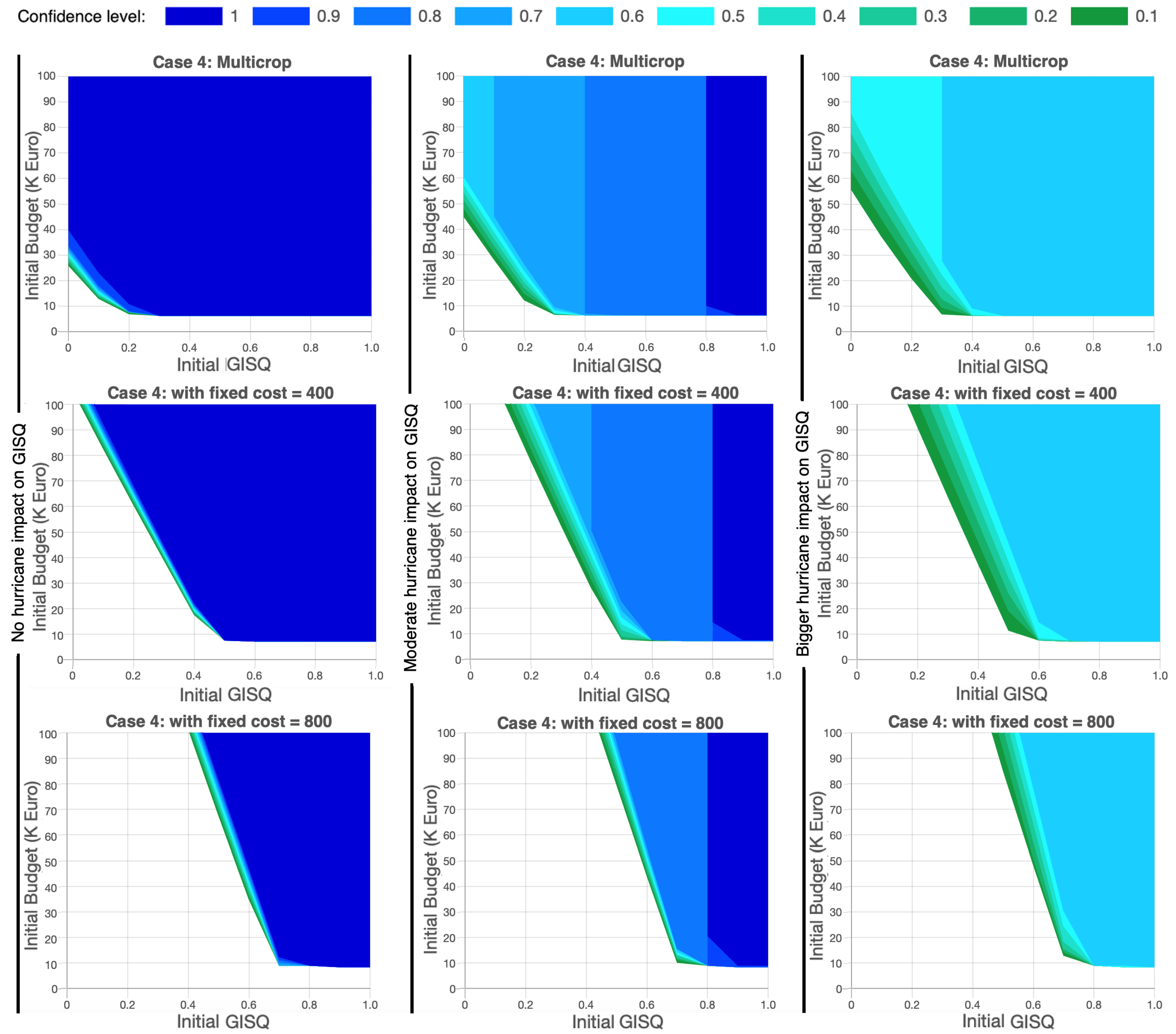
6.1.4. Impact of Fixed Charges

Figure 8 displays the capture basins of C4 with different fixed costs (100, 400, and 800) and different hurricane impacts on the GISQ. First, we note that these results are consistent with the conclusions reached in Section 6.1.1. Second, the overall shape of the capture basins remains the same when the fixed cost changes. This means that, if it is possible to reach the target from a certain initial GISQ with a certain probability, then it remains possible to reach it if the fixed cost is increased. However, the minimum budget for restoration significantly changes, i.e., it gets higher for cases with higher fixed costs. Further, the difference in budget when considering two fixed-cost values is more pronounced when the initial GISQ is low. Indeed, if we compare the minimum restoration budgets for the same level of improvement within the same time horizon and with the same probability (Figure 9), we see that the budgets for cases with higher fixed costs are higher than those with lower fixed costs, and also that the budget increment is much larger when the initial GISQ is low. This difference can be explained by the fact that the crops planted in a better quality soil yield more and, therefore, generate more income, which can be used to cover a larger portion of the fixed costs.

Comparing the minimum restoration budget of these three cases for different time horizons (Figure 6), we confirm that the minimum budget increases with the fixed cost. Additionally, we notice that the difference in budgets becomes smaller as the time horizon gets longer. The budget difference gradually decreases and stabilizes after a certain value of time horizon.

6.1.5. Impact of the Initial GISQ

Figure 9 displays the evolution of the minimum budget needed to raise the GISQ by $0.2$ within 20 years and with a probability of $0.8$, as a function of the initial GISQ, for different hurricane impact levels on the GISQ. In a nutshell, a soil quality improvement of the same level does not necessarily require the same budget when the initial GISQ is low or high.

The first two plots in Figure 9, corresponding to no and moderate hurricane impact on the GISQ, show that the higher the initial GISQ, the lower is the restoration cost. The reason is that a crop planted in better soil generates a higher income than a crop grown in poor-quality soil. Consequently, a lower minimum budget is needed, as the income covers a larger portion of the exploitation costs. Note that the budget may be roughly constant regardless of the initial GISQ value, as in C2. This occurs when the crop’s yield is not very sensitive to the GISQ value.

When the hurricane impact on the GISQ is large (lower part of Figure 9), the above result remains valid for mid-interval initial GISQ levels. However, the opposite behavior is observed for values that are either close to 0 or 1. For instance, in C4 and C2, the minimum budget curves are increasing near initial GISQ values of 0 and 1. One explanation for this is that, when the GISQ is too low, the degradation caused by a hurricane, regardless of the storm’s severity, cannot be very high. On the other hand, starting with a soil of medium quality leaves room for improvements that exceed the target, in anticipation of future hurricanes and compensating for their damage. However, if the initial GISQ is too high, then such an opportunity is not available, which increases the farm’s sensitivity to hurricane strikes.

6.2. Viable Evolutions

In this section, we exhibit (viable) solutions with the minimum initial budget that lies on the boundary of capture basins. These solutions are not the result of an optimization of, e.g., income or another criterion, they are simply viable. In the case of multiple solutions, we chose the one with the highest final treasury. Further, we recall that the problem of determining viable evolutions is represented by a decision tree, with each branch corresponding to the evolution of the state for one possible realization of the uncertainties during the exploitation period.

Figure 10 displays one branch of the solution for case C4 over 40 years ($T=480$ months), for a GISQ target $I^{*}=0.8$ with an initial GISQ of $0.6$, and a confidence level $p=0.8$. The upper part of the figure shows the evolution of the GISQ and the treasury over the time horizon, while the lower part exhibits the sequence of controls to apply. Finally, the red vertical lines indicate the instants of the hurricane’s strikes and their intensity (“m” stands for a minor hurricane and “M” for a major one).

A first observation is that each increase in the treasury comes with a decrease of the GISQ level and vice versa. This illustrates the conflict between the criteria of farm profitability and resource preservation, which is at the root of our problem. The GISQ level goes from its initial value $I^0$ at time 0 to reach $I^T\ge I^{*}$ at the terminal date. The treasury starts at the minimum restoration budget, goes up and down over time, and remains positive throughout the planning horizon.

We make the following remarks on the viable evolutions and the effect of some parameters:

  

Crop recommendations: in all viable evolutions, there is a prevalence of fallow as a recommended control. This is due to the fact that the solutions lie on the boundary of the capture basin. Even if it were possible to obtain higher revenues by investing a bit more, the algorithm returns the solution with the minimum budget. As the cheapest option is fallow, this is most likely to be chosen.

  

Direct hurricane impact on the GISQ: when the GISQ is more sensitive to hurricane strikes, we once again notice that fallow controls are very prevalent. This is intuitive as they offer the best GISQ improvement to price ratio. When the impact of hurricanes on the GISQ is low, the degradation over time becomes less significant and thus we can afford the use of more profitable crops even if they are less performant on the GISQ improvement side.

  

Time horizon: the impact of the planning horizon depends on the hurricane impact on the GISQ. When this impact is low, fallows are less recommended when the horizon is longer. However, when the direct effect of hurricanes on the GISQ is high, then fallow controls are recommended more often, due to the large accumulation of damage on the GISQ over longer periods of time, as alluded to in Section 6.1.2.

  

Fixed charges: higher fixed costs call for more profitable crops, that is, other than fallow. This is expected, as a higher income helps to cover this cost. In fact, it is more appealing to increase revenues than to keep budget to cover fixed costs. However, this result no longer holds when the hurricane impact on the GISQ is too high. Indeed, in this case, achieving the GISQ target becomes harder, if even possible, using productive crops. Consequently, there may be no other choice than fallow controls to improve the GISQ, which adds the fixed cost to the initial budget.

  

Level of improvement: the comparison of Figure 10, Figure 11 and Figure 12, which respectively show a branch of the feedback solution tree for an initial GISQ of $0.6$, $0.1$, and 1, shows that a higher level of improvement in the GISQ involves a fallow control. The intuition is crystal clear: a small level of improvement in the GISQ requires less effort and time to achieve, which leaves more time to improve the treasury.

7. Conclusions

The main qualitative takeaways of our study are as follows:

• The results seem to be highly sensitive to the direct effect of hurricanes on the GISQ, which in turn strongly affects the impact of the other parameters.
• Cases C1 and C2 are globally less efficient than the others, which suggests that the export-oriented sector is more vulnerable and less resilient to climatic uncertainties than the sector aimed at the local market. This result is quite worrisome, given that the export-oriented sector represents a fairly large portion of the economy of small tropical islands such as Guadeloupe and Martinique.
• Because it conflicts with profitability and food-security objectives, preserving the soil is far from an easy task. This difficulty is accentuated by climatic uncertainties, which are the most damaging hazards to soil preservation, not only in terms of cost, but also due to their direct impact on the soil itself. Our results highlight that restoration possibilities and cost are very sensitive to the direct impact of hurricanes on soil quality. Consequently, it is crucial to have studies assessing the impact of hurricanes on the GISQ (and hence on soil quality).

Future developments include collecting additional data and refining the estimations of hurricane-related parameters (impact on the GISQ, recovery time, cost, and occurrence probabilities). A second interesting extension would be to consider a multi-parcel setting to assess the potential advantages of multi-cropping, both in terms of efficiency and risk management. Finally some cropping systems, such as monocultures, often lead to gradual soil degradation, but this can be decreased or even reversed to a certain extent with no or minimum tillage, cover cropping and organic amendment strategies. It would be then interesting to take into account, in future research, the effect of successive use of the same crop or type of crop *.

* We are grateful to one Reviewer for suggesting this extension.

** We would like to thank three anonymous Reviewers for their very helpful comments.