A Period-Aware Hybrid Model Applied for Forecasting AQI Time Series

Abstract
1. Introduction
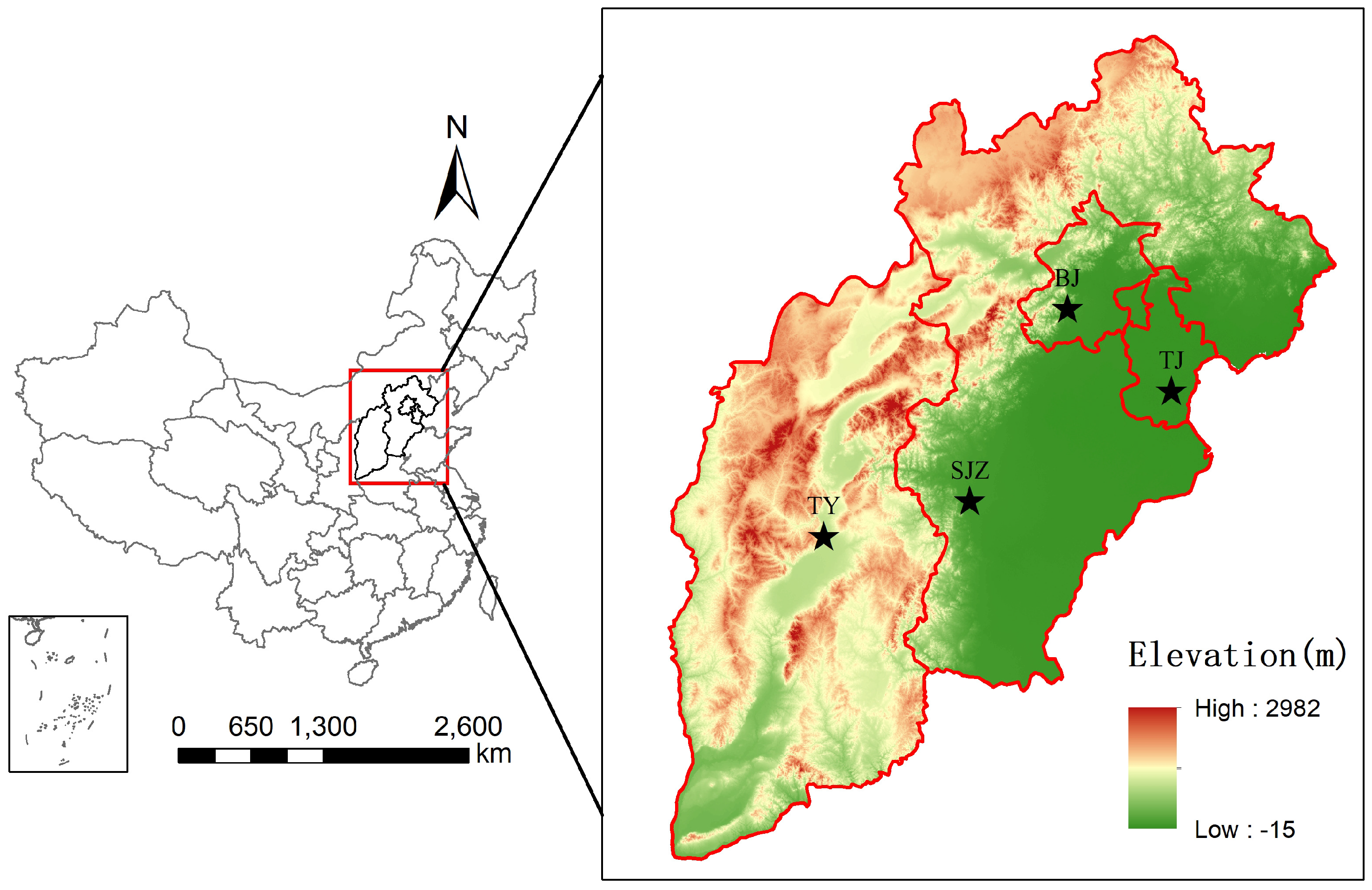
2. Data Description
3. Methods
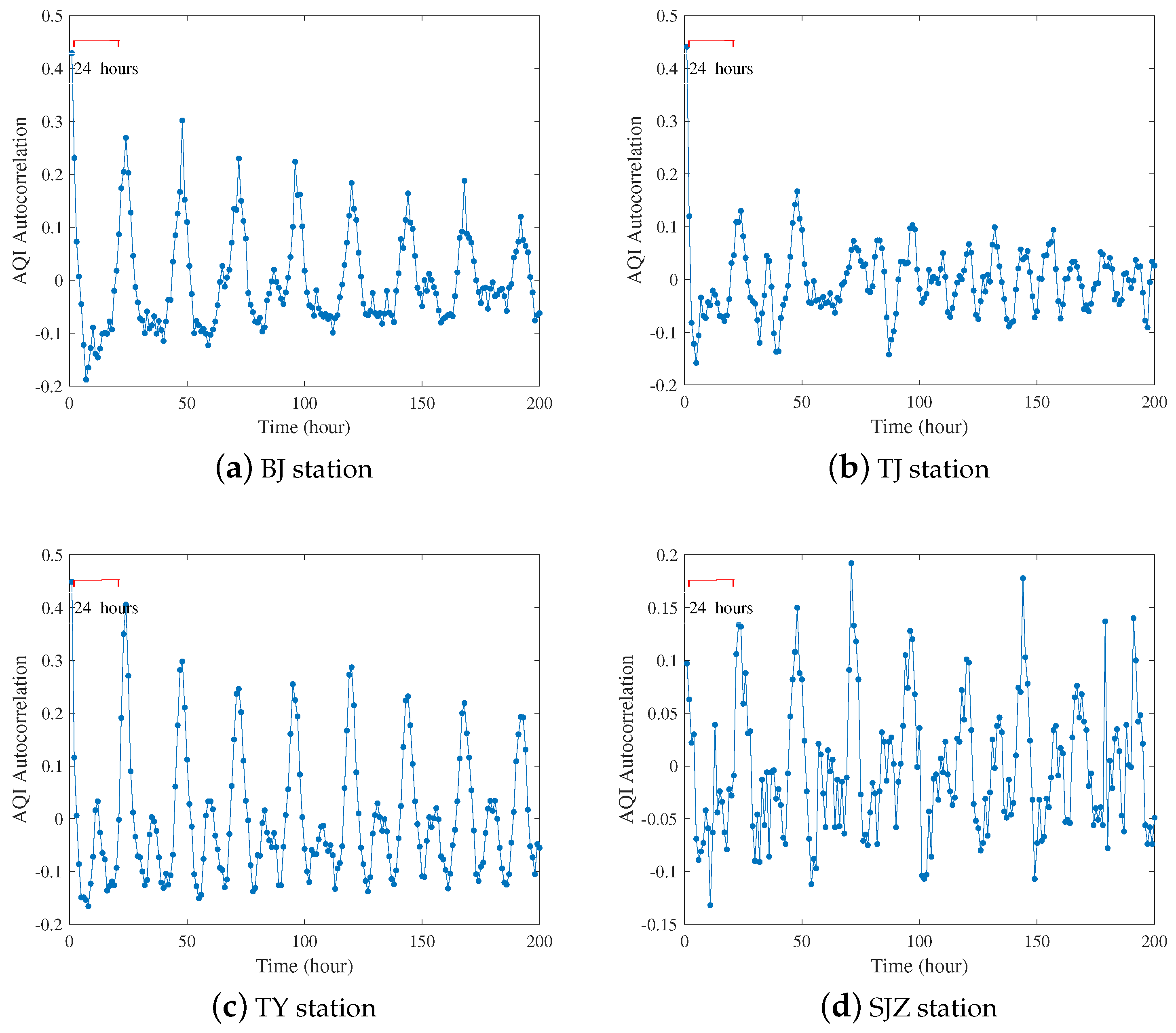
3.1. Period Analysis
3.2. Period Extraction Algorithm Based on Luenberger Observer
3.3. Period-Aware Hybrid Model
3.4. Performance Indices of Model’s Prediction Accuracy
4. Results and Discussion
4.1. Period Analysis Results
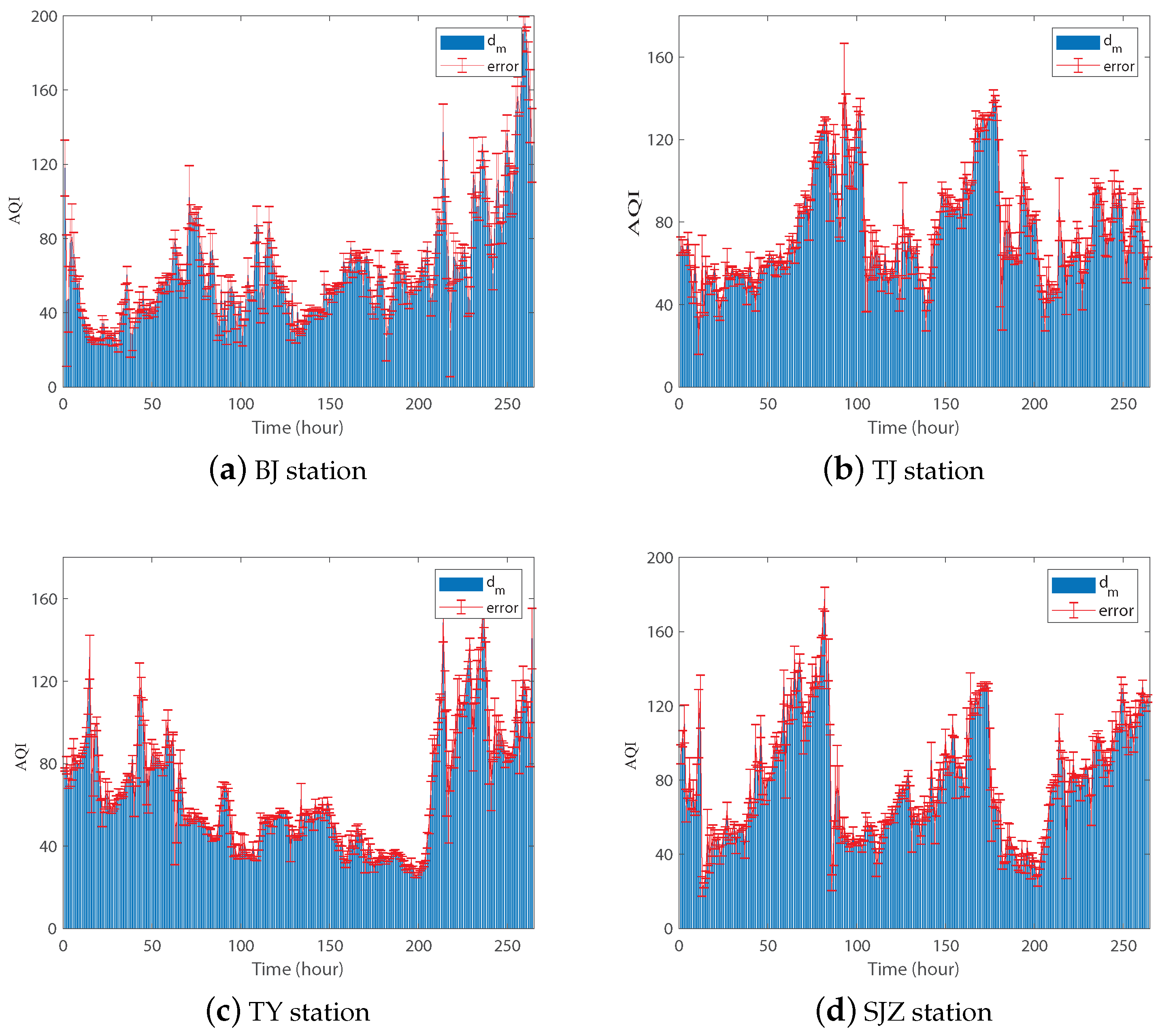
4.2. The Results of Period Extraction Algorithm
4.3. Results of the Period-Aware Hybrid Model
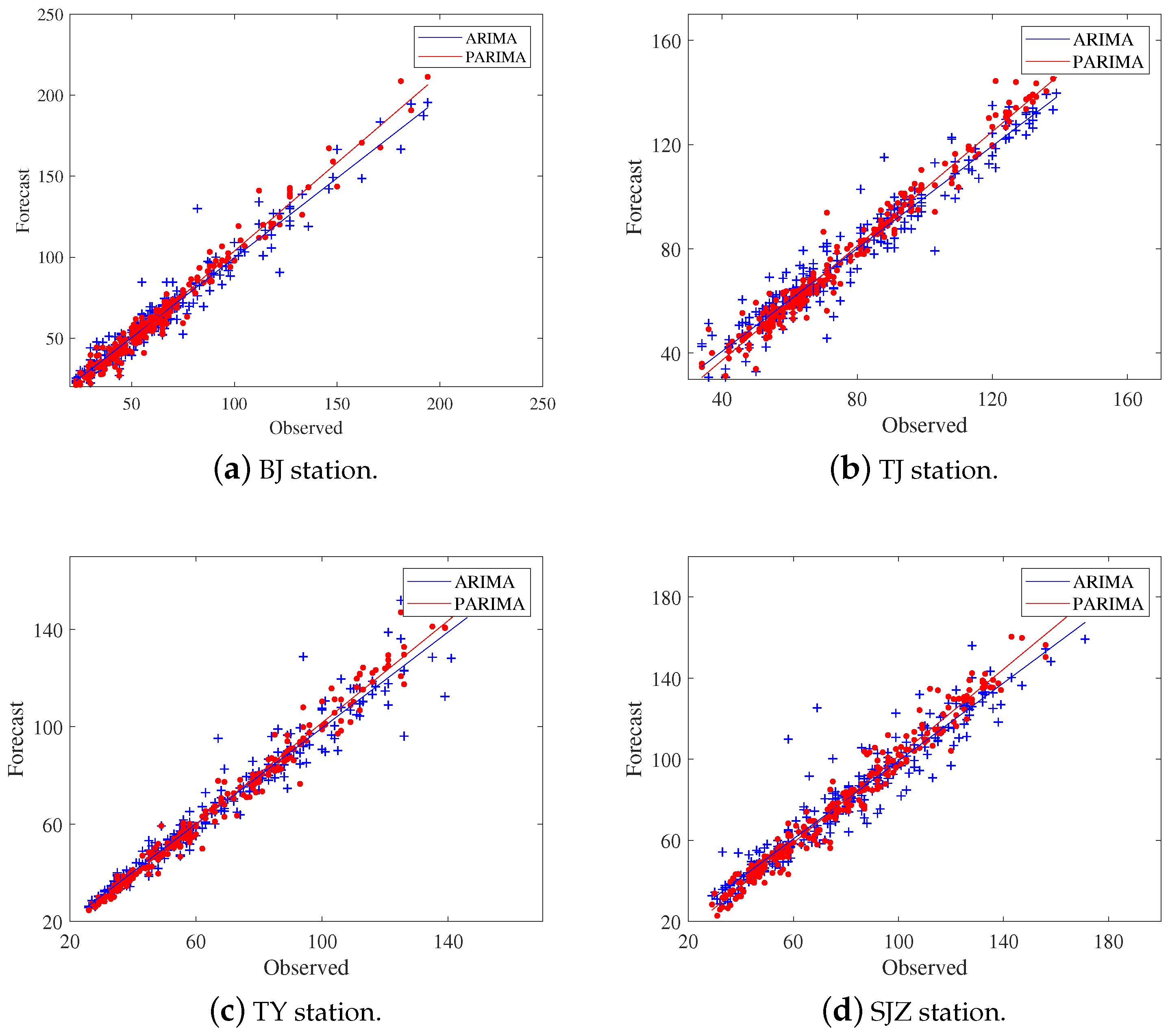
4.3.1. Results of the ARIMA and PARIMA
4.3.2. Results of the ANN and PANN
4.3.3. Results of the SVM and PSVM
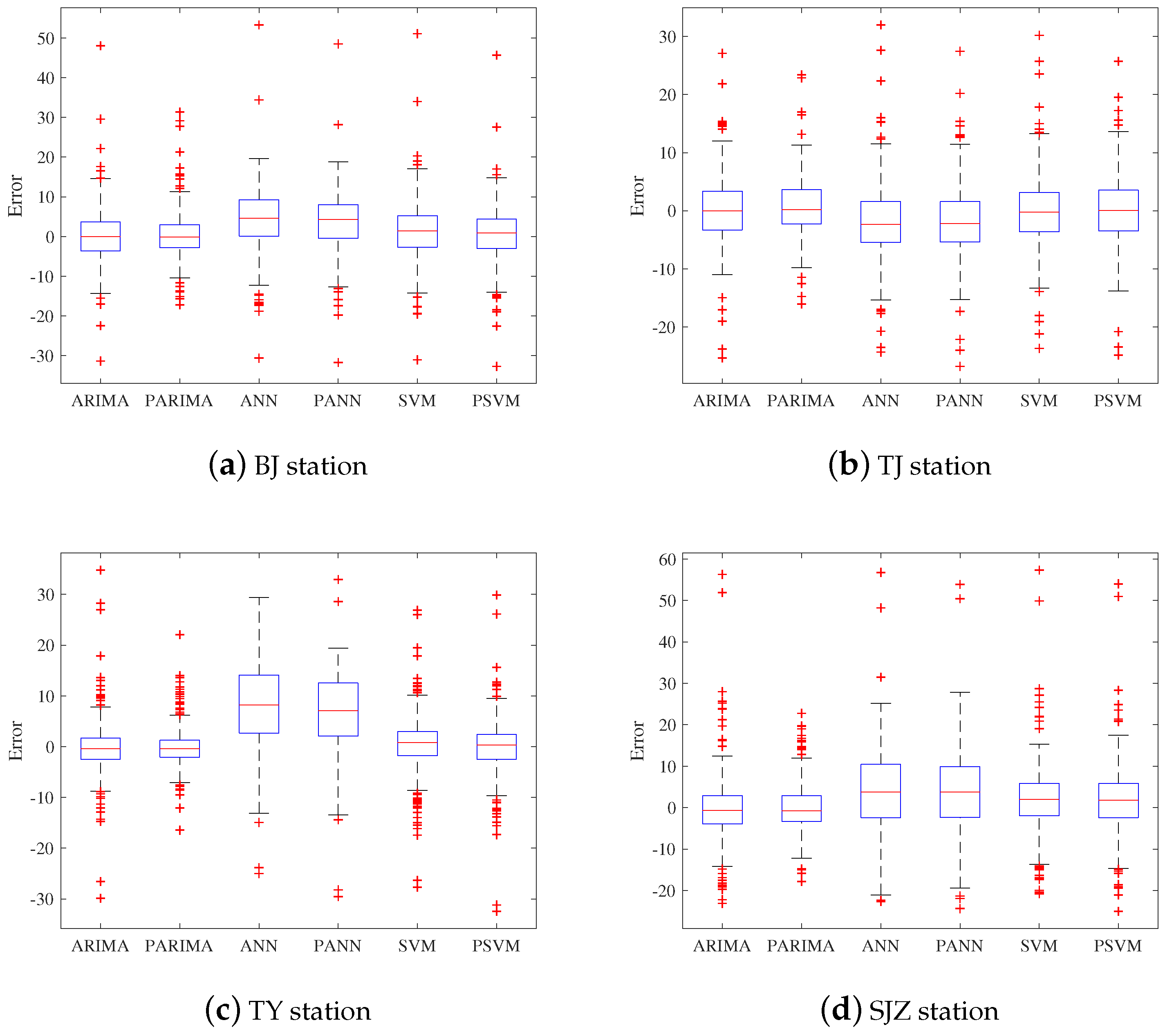
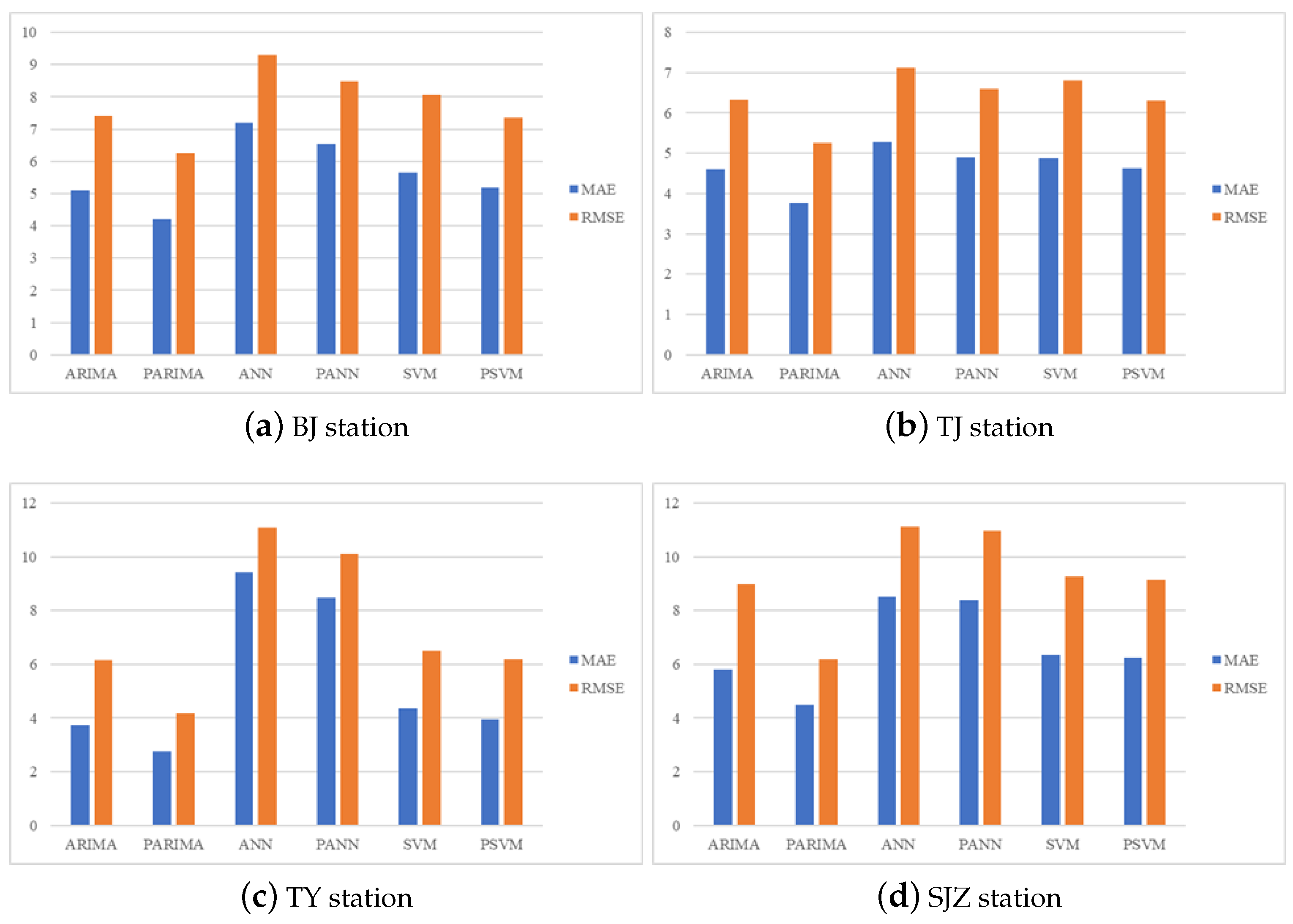
4.3.4. Comparison of Hybrid Models’ Results
5. Conclusions
Author Contributions
Funding
Conflicts of Interest
References
- Wu, Q.; Lin, H. Daily urban air quality index forecasting based on variational mode decomposition, sample entropy and LSTM neural network. Sustain. Cities Soc. 2019, 50, 101657. [Google Scholar] [CrossRef]
- MEE. Ambient Air Quality Standards. (Document GB 3095-2012); Ministry of Ecology and Environment of the People’s Republic of China: Beijing, China, 2012.
- Zhu, S.; Lian, X.; Liu, H.; Hu, J.; Wang, Y.; Che, J. Daily air quality index forecasting with hybrid models: A case in China. Environ. Pollut. 2017, 231, 1232–1244. [Google Scholar] [CrossRef] [PubMed]
- Wang, D.; Wei, S.; Luo, H.; Yue, C.; Grunder, O. A novel hybrid model for air quality index forecasting based on two-phase decomposition technique and modified extreme learning machine. Sci. Total Environ. 2017, 580, 719–733. [Google Scholar] [CrossRef] [PubMed]
- Jiang, F.; He, J.; Tian, T. A clustering-based ensemble approach with improved pigeon-inspired optimization and extreme learning machine for air quality prediction. Appl. Soft Comput. 2019, 85, 105827. [Google Scholar] [CrossRef]
- Wu, Q.; Lin, H. A novel optimal-hybrid model for daily air quality index prediction considering air pollutant factors. Sci. Total Environ. 2019, 683, 808–821. [Google Scholar] [CrossRef] [PubMed]
- Zhu, C.; Fan, R.; Sun, J.; Luo, M.; Zhang, Y. Exploring the fluctuant transmission characteristics of Air Quality Index based on time series network model. Ecol. Indic. 2020, 108, 105681. [Google Scholar] [CrossRef]
- Zhu, S.; Yang, L.; Wang, W.; Liu, X.; Lu, M.; Shen, X. Optimal-combined model for air quality index forecasting: 5 cities in North China. Environ. Pollut. 2018, 243, 842–850. [Google Scholar] [CrossRef] [PubMed]
- Cinar, Y.G.; Mirisaee, H.; Goswami, P.; Gaussier, E.; Aït-Bachir, A. Period-aware content attention RNNs for time series forecasting with missing values. Neurocomputing 2018, 312, 177–186. [Google Scholar] [CrossRef]
- Bernas, M.; Płaczek, B. Period-aware local modelling and data selection for time series prediction. Expert Syst. Appl. 2016, 59, 60–77. [Google Scholar] [CrossRef]
- Sang, Y.F.; Wang, Z.; Liu, C. Period identification in hydrologic time series using empirical mode decomposition and maximum entropy spectral analysis. J. Hydrol. 2012, 424–425, 154–164. [Google Scholar] [CrossRef]
- Xue, J.; Xu, Y.; Zhao, L.; Wang, C.; Rasool, Z.; Ni, M.; Wang, Q.; Li, D. Air pollution option pricing model based on AQI. Atmos. Pollut. Res. 2019, 10, 665–674. [Google Scholar] [CrossRef]
- Zheng, S.; Cao, C.X.; Singh, R.P. Comparison of ground based indices (API and AQI) with satellite based aerosol products. Sci. Total Environ. 2014, 488–489, 398–412. [Google Scholar] [CrossRef] [PubMed]
- Song, Z.; Fu, D.; Zhang, X.; Han, X.; Song, J.; Zhang, J.; Wang, J.; Xia, X. MODIS AOD sampling rate and its effect on PM2.5 estimation in North China. Atmos. Environ. 2019, 209, 14–22. [Google Scholar] [CrossRef]
- Fu, D.; Xia, X.; Wang, J.; Zhang, X.; Li, X.; Liu, J. Synergy of AERONET and MODIS AOD products in the estimation of PM2.5 concentrations in Beijing. Sci. Rep. 2018, 8. [Google Scholar] [CrossRef] [PubMed]
- Box, G. Box and Jenkins: Time Series Analysis, Forecasting and Control; Palgrave Macmillan: London, UK, 2013; pp. 161–215. [Google Scholar]
- Kumar, A.; Goyal, P. Forecasting of daily air quality index in Delhi. Sci. Total Environ. 2011, 409, 5517–5523. [Google Scholar] [CrossRef] [PubMed]
- Maciąg, P.S.; Kasabov, N.; Kryszkiewicz, M.; Bembenik, R. Air pollution prediction with clustering-based ensemble of evolving spiking neural networks and a case study for London area. Environ. Model. Softw. 2019, 118, 262–280. [Google Scholar] [CrossRef]
- Li, H.; Wang, J.; Li, R.; Lu, H. Novel analysis-forecast system based on multi-objective optimization for air quality index. J. Clean. Prod. 2019, 208, 1365–1383. [Google Scholar] [CrossRef]
- Wang, J.; Hu, J. A robust combination approach for short-term wind speed forecasting and analysis—Combination of the ARIMA (Autoregressive Integrated Moving Average), ELM (Extreme Learning Machine), SVM (Support Vector Machine) and LSSVM (Least Square SVM) forecasts using a GPR (Gaussian Process Regression) model. Energy 2015, 93 Pt 1, 41–56. [Google Scholar] [CrossRef]
- Mouatadid, S.; Raj, N.; Deo, R.C.; Adamowski, J.F. Input selection and data-driven model performance optimization to predict the Standardized Precipitation and Evaporation Index in a drought-prone region. Atmos. Res. 2018, 212, 130–149. [Google Scholar] [CrossRef]


| AQI Data | Mean | Median | Maximum | Minimum | Std.dev. | Skewness | Kurtosis | Jarue-Bera | Probability |
|---|---|---|---|---|---|---|---|---|---|
| BJ | 87.31048 | 80.00000 | 204.0000 | 23.00000 | 40.46884 | 0.652530 | 2.757676 | 54.61900 | 0.000000 |
| TJ | 78.71371 | 71.00000 | 153.0000 | 34.00000 | 24.59191 | 0.790826 | 2.786825 | 78.95905 | 0.000000 |
| TY | 89.19355 | 89.00000 | 202.0000 | 26.00000 | 32.47751 | 0.379377 | 3.170667 | 18.74958 | 0.000085 |
| SJZ | 97.21505 | 94.50000 | 202.0000 | 29.00000 | 34.07915 | 0.409457 | 2.908065 | 21.05127 | 0.000027 |
| Require: the AQI time series , where at time i. |
| Ensure: the forecasting value at time . |
| 1: Forming the set based on AQI time series X, where , , we get the training data set for time series forecasting model (ARIMA, ANN and SVM). For ARIMA model, the Akaike’s information criterion (AIC) rule is used to determine the p value representing step size of historical data and the remaining parameters d, q in the model. For ANN and SVM models, the lags of the historical values are determined by the partial autocorrelation function (PACF) value. |
| 2: Applying period extraction algorithm based on Luenberger observer to time series X, the representing period information is obtained. |
| 3: Constructing the new training dataset , where and coming from the previous step, period information is integrated into training data. |
| 4: Similarly, according to the period extraction information, the vector representing the system input at time is built. |
| 5: Training the time series forecasting system on new training set , where the vector represents the input, and is the output of the system, we optimize the relevant parameters of the prediction systems in accordance with the principle of risk minimization. |
| 6: Inputting the feature vector into the trained time series prediction model, the output of the prediction system is the forecasting target at time . |
| Repeat the above steps to obtain the prediction results . |
| AQI Data | ADF | Phillips–Perron | ||||
|---|---|---|---|---|---|---|
| Statistic | Prob. | Test Critical (1%) | Statistic | Prob. | Test Critical (1%) | |
| BJ | −17.29189 * | 0.0000 | −3.438936 | −17.28091 * | 0.0000 | −3.438936 |
| TJ | −15.42580 * | 0.0000 | −3.438960 | −15.41498 * | 0.0000 | −3.438936 |
| TY | −15.83096 * | 0.0000 | −3.438948 | −14.57153 * | 0.0000 | −3.438936 |
| SJZ | −24.68088 * | 0.0000 | −3.438936 | −24.56396 * | 0.0000 | −3.438948 |
| Dataset | Index | ARIMA | PARIMA | ANN | PANN | SVM | PSVM |
|---|---|---|---|---|---|---|---|
| BJ | MAE | 5.1105 | 4.2157 | 7.1994 | 6.5492 | 5.6431 | 5.1685 |
| RMSE | 7.4021 | 6.2486 | 9.3029 | 8.4713 | 8.0574 | 7.3530 | |
| IA | 0.9857 | 0.9907 | 0.9751 | 0.9795 | 0.9824 | 0.9853 | |
| DA | 0.7110 | 0.7909 | 0.5856 | 0.6312 | 0.5741 | 0.6426 | |
| TJ | MAE | 4.5954 | 3.7715 | 5.2852 | 4.8915 | 4.8751 | 4.6354 |
| RMSE | 6.3338 | 5.2479 | 7.1120 | 6.5920 | 6.8099 | 6.3021 | |
| IA | 0.9843 | 0.9902 | 0.9797 | 0.9825 | 0.9807 | 0.9837 | |
| DA | 0.6654 | 0.8137 | 0.5513 | 0.6084 | 0.5741 | 0.6160 | |
| TY | MAE | 3.7335 | 2.7575 | 9.4205 | 8.4716 | 4.3461 | 3.9572 |
| RMSE | 6.1442 | 4.1807 | 11.0859 | 10.1187 | 6.5090 | 6.1880 | |
| IA | 0.9876 | 0.9946 | 0.9522 | 0.9602 | 0.9853 | 0.9867 | |
| DA | 0.7529 | 0.8175 | 0.5970 | 0.6312 | 0.5894 | 0.6274 | |
| SJZ | MAE | 5.7934 | 4.4954 | 8.5069 | 8.3741 | 6.3383 | 6.2472 |
| RMSE | 8.9845 | 6.1776 | 11.1195 | 10.9753 | 9.2624 | 9.1298 | |
| IA | 0.9790 | 0.9909 | 0.9611 | 0.9624 | 0.9757 | 0.9765 | |
| DA | 0.6274 | 0.7757 | 0.6122 | 0.6236 | 0.5932 | 0.6312 |
© 2020 by the authors. Licensee MDPI, Basel, Switzerland. This article is an open access article distributed under the terms and conditions of the Creative Commons Attribution (CC BY) license (http://creativecommons.org/licenses/by/4.0/).
Share and Cite
Wang, P.; Feng, H.; Zhang, G.; Yu, D. A Period-Aware Hybrid Model Applied for Forecasting AQI Time Series. Sustainability 2020, 12, 4730. https://doi.org/10.3390/su12114730
Wang P, Feng H, Zhang G, Yu D. A Period-Aware Hybrid Model Applied for Forecasting AQI Time Series. Sustainability. 2020; 12(11):4730. https://doi.org/10.3390/su12114730
Chicago/Turabian StyleWang, Ping, Hongyinping Feng, Guisheng Zhang, and Daizong Yu. 2020. "A Period-Aware Hybrid Model Applied for Forecasting AQI Time Series" Sustainability 12, no. 11: 4730. https://doi.org/10.3390/su12114730
APA StyleWang, P., Feng, H., Zhang, G., & Yu, D. (2020). A Period-Aware Hybrid Model Applied for Forecasting AQI Time Series. Sustainability, 12(11), 4730. https://doi.org/10.3390/su12114730