
Numerical Study of a Francis Turbine over Wide Operating Range: Some Practical Aspects of Verification


Abstract
1. Introduction
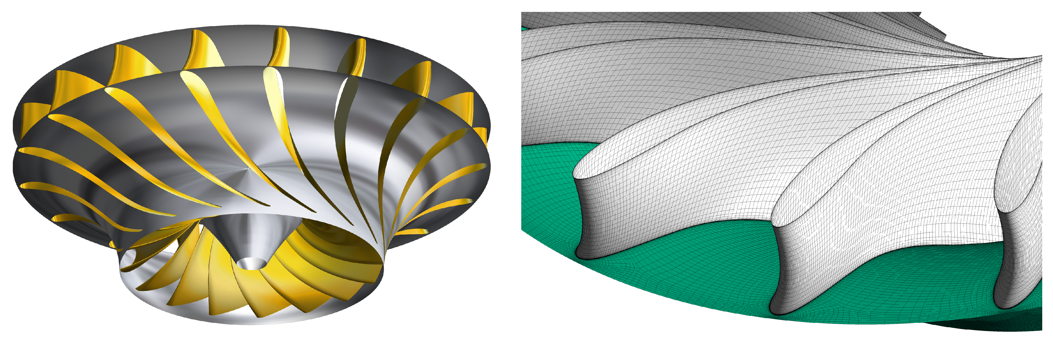
2. Test Case
3. Verification and Validation
4. Conclusions
Author Contributions
Funding
Conflicts of Interest
Abbreviations
| LES | Large eddy simulation |
| RANS | Reynolds-averaged Navier–Stokes equation |
| SAS | Scale adaptive simulation |
| SBES | Stress blended eddy simulation |
| SST | Shear stress transport |
| D | Runner reference diameter (m), m |
| Relative error in efficiency with respect to maximum efficiency | |
| f | Frequency (Hz) |
| g | Gravity (m s−2), m s−2 |
| H | Head (m) |
| N | Number of data points |
| Specific speed, | |
| Specific speed, (rpm, kW, m) | |
| Speed factor | |
| P | Power (W) |
| p | Pressure (Pa) |
| Q | Flow rate (m3 s−1) |
| Discharge factor | |
| s | Runner pitch |
| T | Torque (Nm) |
| t | Time (s) |
| v | Velocity (m s−1) |
| Guide vane opening position (%) | |
| Efficiency | |
| Standard deviation |
Appendix A

| n (rpm) | Q (m3 s−1) | (Pa) | (Pa) | H (m) | T (Nm) | (%) | (°) | ||
|---|---|---|---|---|---|---|---|---|---|
| 0.180 | 0.063 | 531.50 | 0.133 | 355,025 | 60,633 | 29.99 | 603.40 | 86.120 | 3.95 |
| 0.180 | 0.080 | 531.40 | 0.168 | 355,825 | 61,526 | 30.04 | 792.5 | 89.280 | 5.01 |
| 0.180 | 0.095 | 531.40 | 0.199 | 356,325 | 62,523 | 30.03 | 955.5 | 90.970 | 6.02 |
| 0.180 | 0.110 | 531.40 | 0.230 | 353,725 | 60,322 | 30.06 | 1126.10 | 92.290 | 6.99 |
| 0.180 | 0.125 | 531.50 | 0.261 | 353,625 | 61,310 | 30.02 | 1288.90 | 93.230 | 8.00 |
| 0.180 | 0.139 | 531.40 | 0.291 | 353,725 | 62,217 | 30.01 | 1436.90 | 93.470 | 9.01 |
| 0.180 | 0.153 | 531.50 | 0.319 | 350,725 | 60,143 | 30.00 | 1578.40 | 93.520 | 10.02 |
| 0.180 | 0.166 | 531.60 | 0.347 | 352,025 | 62,756 | 30.02 | 1710.60 | 93.160 | 10.99 |
| 0.180 | 0.179 | 531.60 | 0.374 | 349,825 | 60,740 | 30.09 | 1843.80 | 92.970 | 12.00 |
| 0.180 | 0.191 | 531.70 | 0.399 | 348,925 | 61,145 | 30.04 | 1952.30 | 92.400 | 13.05 |
| 0.180 | 0.202 | 531.70 | 0.423 | 348,325 | 61,549 | 30.03 | 2054.20 | 91.760 | 14.02 |
| n (rpm) | Q (m3 s−1) | (Pa) | (Pa) | H (m) | T (Nm) | (%) | (°) | ||
|---|---|---|---|---|---|---|---|---|---|
| 0.180 | 0.057 | 531.50 | 0.118 | 353,840 | 60,579 | 29.98 | 549.87 | 88.120 | 3.95 |
| 0.180 | 0.073 | 531.40 | 0.153 | 354,390 | 61,472 | 29.99 | 722.04 | 90.638 | 5.01 |
| 0.180 | 0.087 | 531.40 | 0.181 | 354,400 | 62,508 | 29.93 | 879.27 | 92.137 | 6.02 |
| 0.180 | 0.100 | 531.40 | 0.209 | 351,120 | 60,390 | 29.86 | 1020.40 | 92.662 | 6.99 |
| 0.180 | 0.113 | 531.50 | 0.237 | 349,950 | 61,536 | 29.98 | 1247.70 | 92.625 | 8.00 |
| 0.180 | 0.130 | 531.40 | 0.272 | 348,800 | 62,658 | 29.91 | 1353.40 | 92.095 | 9.01 |
| 0.180 | 0.148 | 531.50 | 0.310 | 371,850 | 59,703 | 30.01 | 1530.00 | 95.309 | 10.02 |
| 0.180 | 0.156 | 531.60 | 0.326 | 350,450 | 62,288 | 29.89 | 1641.90 | 95.295 | 10.99 |
| 0.180 | 0.169 | 531.60 | 0.352 | 348,000 | 60,145 | 29.94 | 1771.20 | 95.148 | 12.00 |
| 0.181 | 0.180 | 531.70 | 0.374 | 346,090 | 60,756 | 29.75 | 1838.10 | 93.906 | 13.05 |
| 0.181 | 0.191 | 531.70 | 0.397 | 345,390 | 61,150 | 29.72 | 1930.70 | 93.008 | 14.02 |
References
- Iliev, I.; Trivedi, C.; Dahlhaug, O.G. Variable-speed operation of Francis turbines: A review of the perspectives and challenges. Renew. Sustain. Energy Rev. 2019, 103, 109–121. [Google Scholar] [CrossRef]
- Quaranta, E. Optimal rotational speed of Kaplan and Francis turbines with focus on low-head hydropower applications and dataset collection. J. Hydraul. Eng. 2019, 145, 1–15. [Google Scholar] [CrossRef]
- Quaranta, E.; Muller, G. Optimization of undershot water wheels in very low and variable flow rate applications. J. Hydraul. Res. 2020, 58, 1–5. [Google Scholar] [CrossRef]
- Keck, H.; Sick, M. Thirty years of numerical flow simulation in hydraulic turbomachines. Acta Mech. 2008, 201, 211–229. [Google Scholar] [CrossRef]
- Celik, I.B.; Ghia, U.; Roache, P.J.; Freitas, C.J. Procedure for estimation and reporting of uncertainty due to discretization in CFD applications. J. Fluids Eng. 2008, 130, 078001. [Google Scholar] [CrossRef]
- Roache, P. Perspective: Validation—What does it mean? J. Fluids Eng. 2009, 131, 034503. [Google Scholar] [CrossRef]
- Roy, C.; Oberkampf, W. A comprehensive framework for verification, validation, and uncertainty quantification in scientific computing. Comput. Method Appl. Mech. Eng. 2011, 200, 2131–2144. [Google Scholar] [CrossRef]
- Cervantes, M.J.; Trivedi, C.; Dahlhaug, O.G.; Nielsen, T.K. Francis-99 Workshop 1: Steady operation of Francis turbines. J. Phys. Conf. Ser. 2015, 579, 011001. [Google Scholar] [CrossRef]
- Trivedi, C.; Cervantes, M.J.; Dahlhaug, O.G. Experimental and numerical studies of a high-head Francis turbine: A review of the Francis-99 test case. Energies 2016, 9, 74. [Google Scholar] [CrossRef]
- Trivedi, C.; Cervantes, M.J.; Dahlhaug, O.G. Numerical techniques applied to hydraulic turbines: A perspective review. Appl. Mech. Rev. 2016, 68, 010802. [Google Scholar] [CrossRef]
- Trivedi, C.; Cervantes, M.J. Fluid-structure interactions in Francis turbines: A perspective review. Renew. Sustain. Energy Rev. 2017, 68, 87–101. [Google Scholar] [CrossRef]
- Trivedi, C. A review on fluid structure interaction in hydraulic turbines: A focus on hydrodynamic damping. Eng. Fail. Anal. 2017, 77, 1–22. [Google Scholar] [CrossRef]
- Trivedi, C. Investigations of compressible turbulent flow in a high-head Francis turbine. J. Fluids Eng. 2018, 140, 011101. [Google Scholar] [CrossRef]
- Trivedi, C. A systematic validation of a Francis turbine under design and off-design loads. J. Verif. Valid. Uncertain. Quantif. 2019, 4, 011003. [Google Scholar] [CrossRef]
- Trivedi, C.; Dahlhaug, O.G. A comprehensive review of verification and validation techniques applied to hydraulic turbines. Int. J. Fluid Mach. Syst. 2019, 12, 345–367. [Google Scholar] [CrossRef]
- Trivedi, C.; Agnalt, E.; Dahlhaug, O.G. Experimental study of a Francis turbine under variable-speed and discharge conditions. Renew. Energy 2018, 119, 447–458. [Google Scholar] [CrossRef]


| Parameters | Description |
|---|---|
| Mesh | spiral casing—3.56 million, guide vanes—4.75 million, |
| runner—5.63 million, draft tube—2.9 million. | |
| Boundary types | Total pressure inlet and static pressure outlet |
| Turbulence model | SAS-SST |
| Advection scheme | High Resolution |
| Time marching scheme | Second order backward Euler |
| Time | Time step: 1° of runner rotation. Total time: three rotations |
© 2020 by the authors. Licensee MDPI, Basel, Switzerland. This article is an open access article distributed under the terms and conditions of the Creative Commons Attribution (CC BY) license (http://creativecommons.org/licenses/by/4.0/).
Share and Cite
Trivedi, C.; Iliev, I.; Dahlhaug, O.G. Numerical Study of a Francis Turbine over Wide Operating Range: Some Practical Aspects of Verification. Sustainability 2020, 12, 4301. https://doi.org/10.3390/su12104301
Trivedi C, Iliev I, Dahlhaug OG. Numerical Study of a Francis Turbine over Wide Operating Range: Some Practical Aspects of Verification. Sustainability. 2020; 12(10):4301. https://doi.org/10.3390/su12104301
Chicago/Turabian StyleTrivedi, Chirag, Igor Iliev, and Ole Gunnar Dahlhaug. 2020. "Numerical Study of a Francis Turbine over Wide Operating Range: Some Practical Aspects of Verification" Sustainability 12, no. 10: 4301. https://doi.org/10.3390/su12104301
APA StyleTrivedi, C., Iliev, I., & Dahlhaug, O. G. (2020). Numerical Study of a Francis Turbine over Wide Operating Range: Some Practical Aspects of Verification. Sustainability, 12(10), 4301. https://doi.org/10.3390/su12104301