Natural Light Influence on Intellectual Performance. A Case Study on University Students

Abstract

Natural light in interior spaces has many advantages: the most obvious is energy savings, but also many long term physical and mental health benefits. Published research demonstrates the positive effects of natural light, especially in spaces used in long term periods, such as offices, houses, hospital rooms, etc. However, how would the deprivation of natural light affect users in spaces of more occasional use, such as lecture theatres, surgery rooms, courtrooms…? The present research consists in a case study that adds some data on that question. The experiment processed the data on the performance of 278 university students in one theoretical course, consisting in three-hour weekly lectures. This course was taught six times, in six consecutive years (2013–2018), three in exclusively artificially lit basement classrooms, and the other three in classrooms with windows, mixing natural and artificial light. The data of the exam and attendance scores were compared statistically for both populations (basement vs. windows classrooms). The research found strong evidence of the classrooms with windows having better exam scores than those in the basement, with mean differences between 13.17% and 7.73%. Mann–Whitney U tests supported this result, with p-values ranging between p << 0.001 and p = 0.007. Attendance differences were not significant.

1. Introduction

Natural lighting in interior spaces is an excellent way of reducing energy costs. Beyond energy savings, natural light has an array of physical and mental health benefits. These two facts are gaining the attention of technical literature related to architectural design. Robinson [1] advocated as long ago as in 1963 for the balanced use of natural and artificial light, stressing the economic use of energy, although he did not elaborate much on the qualities of natural light. Today space design pays more attention to the qualities of natural light: Boubekri’s “Daylight Design” handbook [2] devotes 19 pages to literary evidence on the benefits of natural light, in terms of productivity for office workers, better sales results in commercial spaces, and the long term health benefits of exposure to natural light, as well as problems related to long term deprivation of it. Webb [3] summarized a complete study of these effects in the human body. Boyce [4] collected data from 76 references treating the same subjects as Webb above, comparing the effects of natural light, with the artificial imitations of it by fluorescent and LED lamps, concluding that still more attention to natural daylight in building design is needed. The LEED (Leadership in Energy and Environmental Design) building sustainability assessment method [5], in its latest version, puts emphasis on the benefits of natural light, especially in spaces with long term occupancy, not only for energy savings but also for improved wellbeing and the positive feeling of having exterior views, providing guidelines for correct design (adequate lighting levels, user adjustability, reduction of glare, etc.). However, the implementation of these guidelines is not always easy, and some post occupancy reports demonstrate difficulties to reach the intended visual comfort [6]. Kralikova et al. [7] discussed recent standards improvements consisting of the inclusion of natural light in their requirements, but advocated for a deeper study of its use and effects. Case studies in the literature about office spaces [8,9,10], educational buildings [6], residential spaces [11], and health facilities [12] agree on the long term benefits of the availability of natural light, showing results mainly based on the subjective evaluation of users feelings and preferences, without providing an objective, quantitative result which can be compared among them. They presuppose productivity and performance gains in the users, but these are not objectively quantified. Robinson [1] gave some examples of improvements in productivity in manufacturing spaces in the UK thanks to upgrades in lighting environment, although unfortunately, he focused only on quantitative illuminance levels. Quartier et al. [13] simulated buyers behavior in different shopping lighting conditions. The volunteers of the study felt the mood differences of the diverse light simulations, but the result had little practical result. The Heshong Mahone Group report “Skylighting and Retail Sales” [14] provided objective results of the benefits of natural light in real life activity. The report concluded that in skylit shops, sales could improve between 31% and 49%, compared with those lit with full spectrum fluorescent light (FSFL), that is, fluorescent light of perceptual appearance similar to daylight. It is interesting to note that the users were not aware of which lighting system was used in each space, and that the behavioral change happened during the short time span of the shopping activity (as opposed to the long term exposures considered in previous references). Education is another activity where numerical assessment of the improvements in behavior or productivity is possible, and there are some interesting studies worth noting. Larson [15] compared the output of two K-3 schools (test and control) in the US, where for a period of one year, the windows were removed in the test school. During this period, the lighting was exclusively artificial. The study concluded without finding significant differences between windows and windowless classrooms, neither in exam scores or attendance. Its only recommendation was the provision of adequate light and ventilation levels. The question that motivated that experiment was: If we can provide artificial light and air conditioning, why do we need windows? The reply: only when views are needed. Hathaway [16] published in 1992 the results of a two year long experiment carried out in five elementary schools in Alberta, Canada. He tested the effects of four different kinds of artificial light in students. The conclusion was that the light differences had great influence in the physical and mental development of the children. Among all the tested systems, UV (ultraviolet) emission enhanced FSFL produced the largest benefits in all aspects (health, physical development, attendance, academic achievements). It is not clear that in all cases, artificial light was used exclusively (windows were only mentioned in one of the four settings), but some researchers saw this study as a decided support to the use of FSFL against natural light [17]. In 2001, McColl and Veitech [18] reviewed data from 1941 to 1999 to test the supposed benefits of FSFL over standard fluorescent lights, and found no evidence supporting it. Pullay and Williamson [19] compared the behavior of pre-K1 children under FSFL and LED lights, concluding a clear advantage of LED. Unfortunately, there was no comparison of LED against natural light, and at this moment, LED lighting in classrooms is still not widely experimented. Niklas and Bailey [17] published a paper opposing the aforementioned enthusiastic support of FSFL by Hathaway, demonstrating through a new experiment the rotund advantage of natural light classrooms over those lit exclusively with FSFL. They compared the academic results of three daylit schools in North Carolina (USA) during one to three years (the schools were built in different years) with non-daylit schools. Daylit schools consistently achieved scores between 4% to 14% higher than their counterparts. In 1999, the Heshong Mahone Group released the “Daylighting in Schools” report [20], providing further evidence of the clear benefit of natural light in schools. The most extensive study among the reviewed here, it analyzed the data of 20,000 students attending first to fifth elementary school grades in three districts of California, in over 2000 different classrooms. It demonstrated faster learning and higher grades in the classrooms with more natural light. In the district where normalized exams scores were used, classrooms with the most natural light had scores between 7% to 18% higher than those with the least.

In this context, it seems there is a growing consensus on the benefit of natural light in interior spaces used in the long term, both through subjective appreciations, and by objective numerical results. The standard artificial light, FSFL, compares poorly with natural light. However, what happens in short term used spaces, where intense intellectual activity is needed? Lecture theatres, surgery rooms, courtrooms, and similar spaces are often artificially lit. Their use is occasional or comparatively short, but needs intense intellectual concentration. Would they benefit from natural light, or would its effect be irrelevant?

A fortunate coincidence can shed some data over this question. The author of the present article had the experience of teaching the same course during six consecutive years in the Department of Architecture of Korea University, in Seoul (Korea) [21], three of them in exclusively artificially lit underground rooms, and the other three in classrooms with combined natural and artificial light. The fact of the subjects of the study being university senior students, instead of the usual elementary school students, and the setting in Korea instead of the UK or US, add the interest of testing the hypothesis in a different context. As a case study, it has several advantages: 1. the data are objective and taken from real life activity (as opposed to subjective Likert scale surveys, or experiments based on simulations); 2. the sample of population is large enough to draw significant conclusions, but still homogenous enough to be consistent; 3. the repetition of the experiment three times in both the test group (basement with artificial light) and control group (classrooms with windows) allows us to check for differences between individual years changing circumstances. However, the case study has also obvious limitations: 1. it is very specific; 2. there are clear year by year variations, and 3. it is not possible to achieve perfect symmetry between the populations tested. Notwithstanding these limitations, the present case adds new data to the existing literature, supporting the use of natural light. The next chapter details the design of the experiment, and details its methodology.

2. Materials and Methods

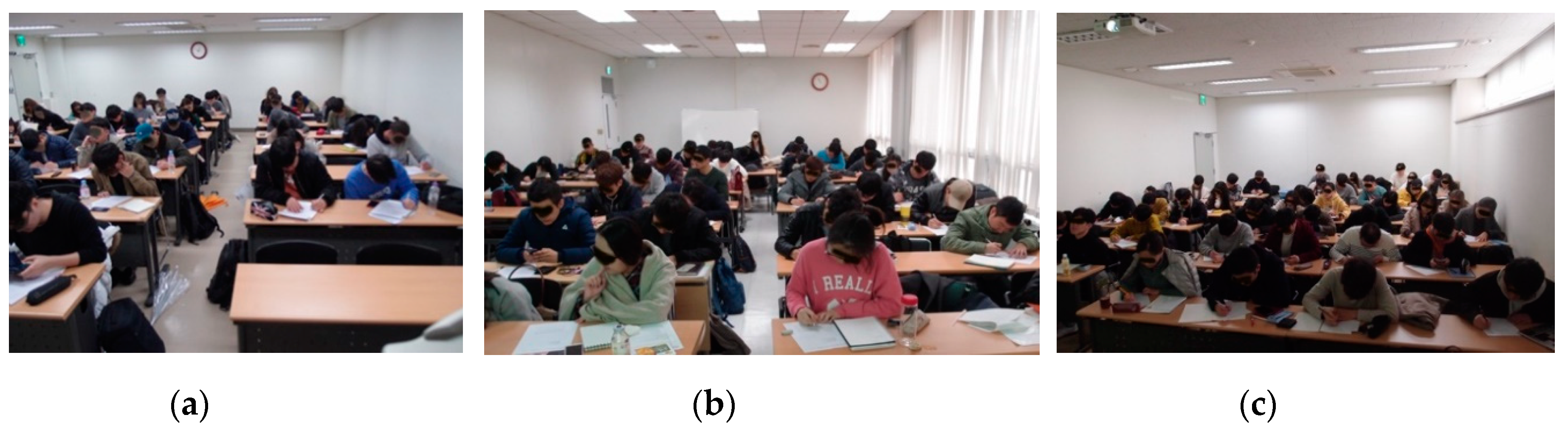
2.1. Population and Distribution

The experiment is performed over the data accumulated on the performance of a total of 278 students of architecture in one specific fifth year theoretical course (Building Systems) [22], which was taught six times, in six consecutive years (2013 to 2018). The fact that in three of the six years, the classes were performed in underground classrooms without natural light provided a good opportunity to test their academic performance against the control group of students that received lessons in classrooms with natural light. The subjects of the experiment represent a fairly homogenous population, as they all belong to the same University and College, and belong to the same age group, all senior undergraduate students, ranging between 22 and 27 years of age (this date is estimated as the university does not disclose the age of students, due to privacy issues). In order to check for possible demographic distortions in the results, the size of classes and the proportion of male versus female students have also been considered for additional testing, as these parameters present noticeable variation between years.

The detailed distribution of students by year, sex, female vs. male ratio, and their belonging to the control group (classroom with windows, henceforth the “windows” group) or the experimental group (henceforth the “basement” group), is detailed in

Table 1. Distribution of students by years, and by “basement” or “windows” classrooms.

Year	Classroom	Female (F)	Male (M)	F Ratio	M Ratio	Total
2013	Basement	25	34	0.43	0.57	59
2015	Basement	20	22	0.39	0.61	42
2018	Basement	21	34	0.48	0.52	55
	Tot. Basement	66	90	0.42	0.58	156
2014	Windows	12	19	0.21	0.79	31
2016	Windows	10	38	0.35	0.65	48
2017	Windows 1	15	28	0.38	0.62	43
	Tot. Windows	37	85	0.30	0.70	122
	Total Students	103	175	0.37	0.63	278

¹ 2017 classroom had clerestory windows open to a light well, with natural light, but not views.

.

2.2. Environment

The classes were performed in the same campus, and in the same semester (all between March and June), therefore no geographical or climatic variations are significant for the purpose of this study. The classes were always performed in the same time interval, from 9:00 a.m. to 11:40 a.m.

All classrooms were lit by full spectrum fluorescent lamps (FSFL): Phillips Cool Daylight 6500 K, adequate for offices and classroom according to Phillips catalogue [23]. This kind of lamps is designed to get as close as possible to the perceptual feeling of natural light. Although the interest of this research focuses on the quality of light, not its quantitative aspects, an approximate measurement of the illuminance (the amount of light per unit of area of working space, in this case, desk surface) was made to check its adequacy. In all cases, it was possible to measure about 500 lux. The rooms with windows had additional natural light, and were provided with curtains to control and diffuse its incidence. Figure 1a–c show respectively the aspect of the basement classroom (2013, 2015 and 2018), the windows classroom (of 2014 and 2016), and the classroom of 2017, with clerestory windows and natural light.

There is no detailed study of the air quality and thermal comfort inside each type of room. This may be considered a limitation of the present research. However, the most obvious difference was the quality of light, as the interior conditioning was reasonably adequate. All classrooms had mechanical ventilation, and air cooling and heating. In windows classrooms of 2014 and 2016, cooling and heating were centralized and provided by window fan-coils with the only control over the fan intensity. Basement and 2017 classrooms were provided with ceiling cassettes and more sophisticated individual controls for temperature and fan intensity. Classrooms with windows (except for 2017) allowed also for additional natural ventilation, as the windows were manually operable, although due to energy saving policies, they were seldom opened. No complaints were received in terms of interior temperature environment or ventilation.

2.3. Course and Parameters Used in the Experiment

The course was performed weekly, during morning time, in two 75 min periods with a 15 min break in between (9:00 a.m. to 10:10 a.m.; 10:30 a.m. to 11:40 a.m.). The course span was of 16 weeks, meaning it had a total of 16 sessions. The contents and teaching methodology were the same during the six years of the experiment, except for minor updates necessary in technical contents. The course was very intensive, as it was planned as a review of all architectural technologies studied in the previous four years, including structural and environmental systems, construction detailing and sustainability issues, and the way of integrating them in the students’ graduation project the following semester. The wide contests, combined with the fact of the course being taught in English, created an intellectually challenging task. Students were required to have full concentration during the whole period, as otherwise they would lose the flow of fairly complex explanations, and have difficulty to follow the remaining contents.

From the course data, the present research focuses primarily on the output or the objective result of each student, as reflected in the exam score (henceforth the “exam”). The exam format and kind of questions (multi selection type, to allow for a clear and non-biased, objective numerical evaluation) were the same for the six years, therefore, the scores are perfectly comparable between populations. The exam was always performed in the same classroom as the lectures. The exam score is therefore used as the parameter that determines in a quantitative and objective way the performance of students under different light conditions. Secondarily, attendance and participation in class (henceforth, “attendance”) is also used as an objective parameter, easy to compare among groups. Attendance score included delays, and also in class distractions, as for example, failing to complete small tasks performed during the lectures. This parameter is included as a way to check if the different light conditions had additional influence beyond the activity in class time, as more absences and delays might mean health issues or less motivation to attend.

2.4. Process and Calculations

This chapter describes the process, and briefly, the methods used in the calculations.

The first step compared the totality of the population of the six courses in the following way:

• The exam score of the whole population of the control group (windows) against the experiment group (basement).
• The attendance score in the same way as “1” above.

For a better understanding of the distribution of both populations, and an easier visualization of data, a PDF (Probability Density Function) was calculated using the Kernel Density Estimation method, and both the PDF and the histogram were graphically plotted [24] (pages 8–9), [25] (Chapter 6). These graphs let us better understand how the results of each group are distributed, and allow for a fast visual comparison of both: if one group is clearly performing better than the other. A Mann–Whitney U Test was used to know if the basement group results will be similar to the window group (what is called the null hypothesis or H0), or if the window group will have a better score than the basement group (the alternative hypothesis or H1), with a more precise estimation of the statistical significance of the differences [26]. This test calculation produces a p-value, where a result of p ≤ 0.05, confirms the alternative hypothesis. This process was done with both the exam and the attendance scores.

The second step was to check for possible differences between the whole of the male and female population, related to the same parameters as above. This was done through a PDF graph with histograms, followed with a Mann–Whitney U Test of:

• Exam score of female vs. male population, H1 being female exam score will be higher.
• Attendance score of female vs. male population, H1 being female attendance will be better.

The third step checked the possible influence of individual circumstances of each year, first visually through boxplots (graphic diagrams displaying the median, quartiles and outliers of each data set) on the parameters detailed below, to check for the existence or not of clear patterns [27]:

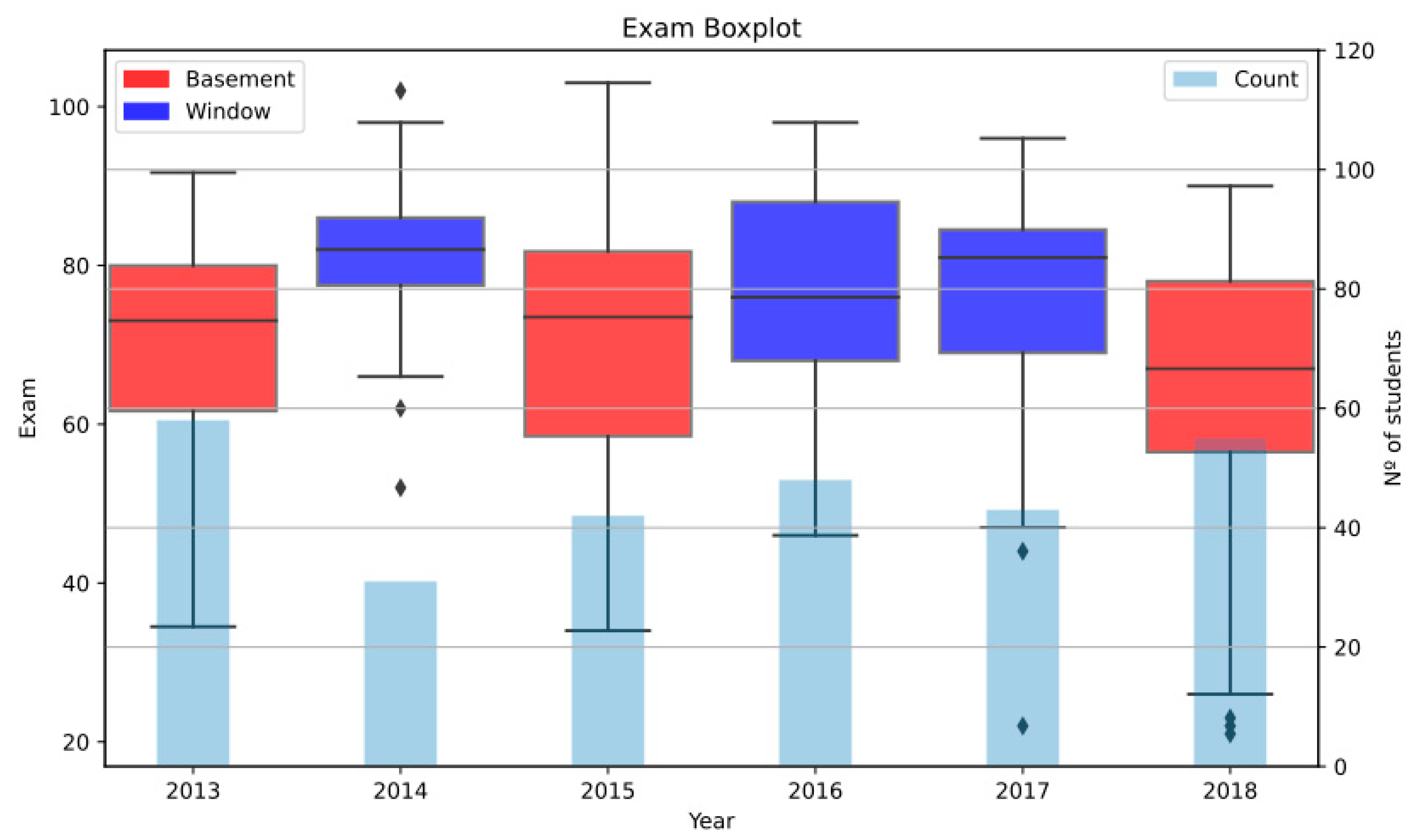
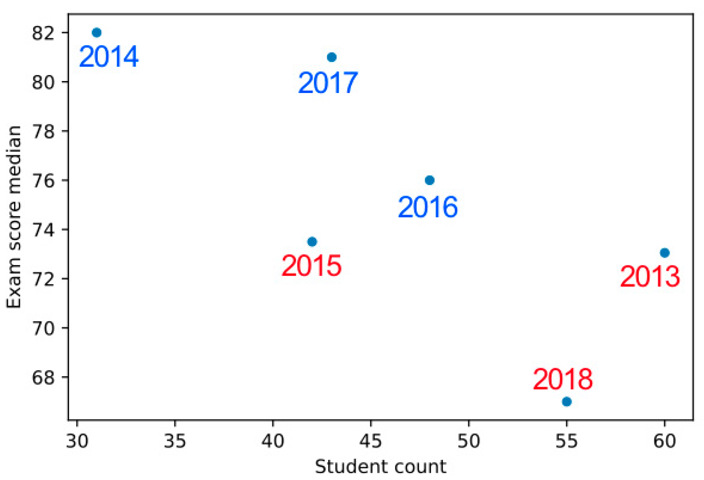
• Exam scores by year, with overlap of the number of students per class.
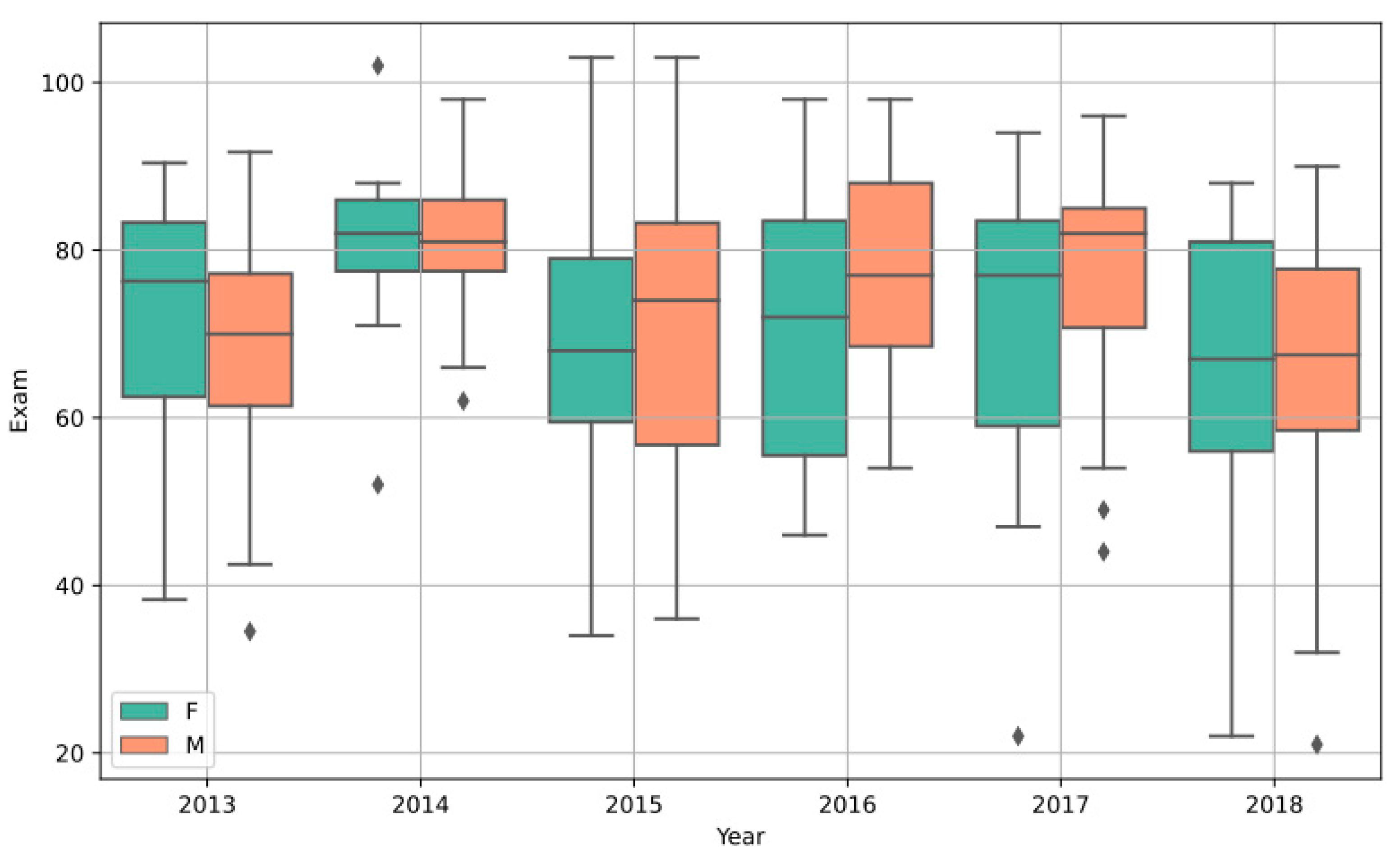
• Exam scores by year, separating male and female populations.
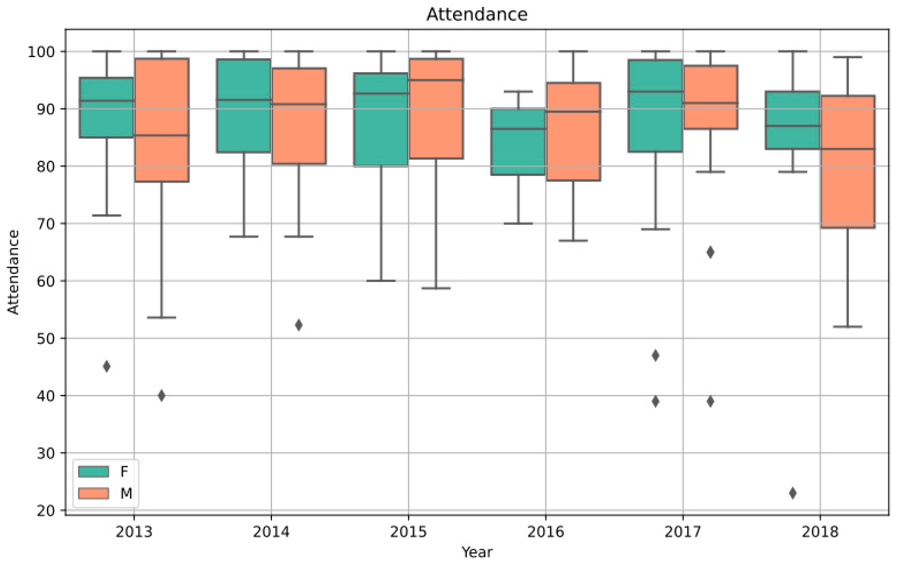
• Same as “2” above, but with the attendance scores.

The fourth step consisted on deciding further PDF graphs and/or Mann–Whitney U Tests by individual years, or by year groups, to reach final conclusions.

All the statistical functions and visualization tools mentioned above (boxplots, Mann–Whitney U Test, PDF graph and the Kernel Density Estimation method used to calculate the PDF) are well known and established, have been briefly described above, and need no further explanation. They were chosen because they are adequate for this kind of study and the size of the population and dataset analyzed.

The statistical calculations were programmed in Python [28], with the use of the SciPy library [29]. The Pandas library for Python was used for the treatment of the raw data tables [30]. The graphics were plotted also on Python with the Seaborn library [31], specifically the functions Distplot, Grouped Boxplots and Annotated Heatmaps. All raw data are available in the Supplementary Materials (see link after Section 4. Conclusions).

3. Results and Discussion

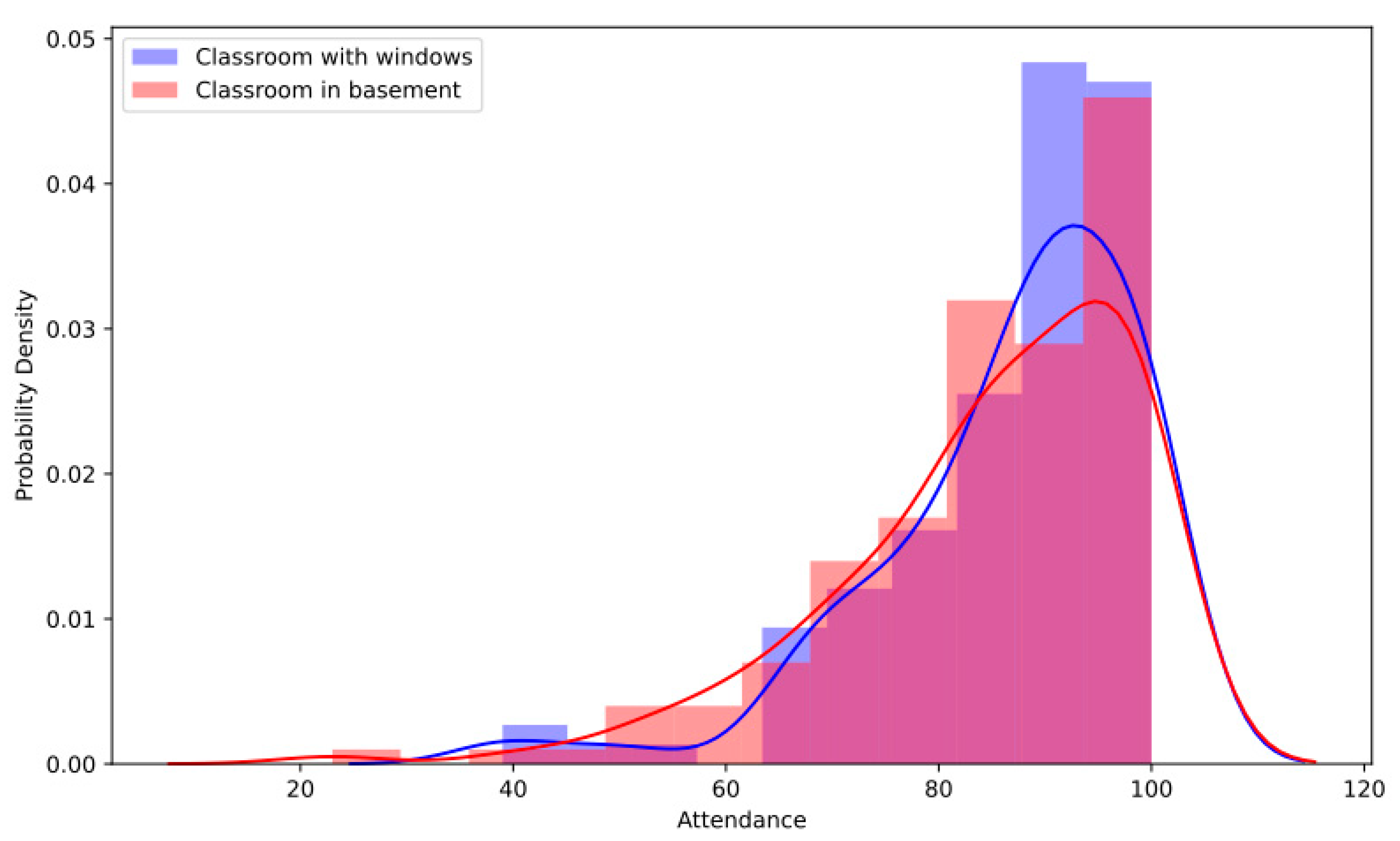
3.1. Step 1. Comparison of the Whole “Windows”vs. “Basement” Populations Regarding Exam and Attendance Score

The PDF graphs with normed histograms of both populations regarding exam and attendance scores are represented in Figure 2 and Figure 3.

The PDF graph shows a clear difference in favor of the “windows” exam, suggesting a strong evidence of the beneficial effect of natural light in the classroom.

In this case, the graph shows the attendance in windows classroom has a higher population in the higher scores, but the distribution curves of both populations are very similar, making it difficult to predict whether one group will perform better than the other.

The key numerical results for both populations, including count, mean value (Mean), standard deviation (Std), minimum, 25%, 50% and 75% quartiles, and maximum, are summarized in

Table 2. Numerical results of “exam” and “attendance” scores of “basement” and “windows” populations.

Parameters	Exam Windows	Exam Basement	Att. Windows	Att. Basement
Count	122	156	122	156
Mean	77.19	68.21	86.93	84.85
Std	13.71	16.90	12.50	14.08
Minimum	22.00	21.00	39.00	23.00
25%	70.00	59.25	80.50	77.90
50%	80.00	70.00	90.00	87.00
75%	86.00	80.00	97.00	96.7
Maximum	102.00	103.00	100.00	100.00

.

The Mann–Whitney U test calculation resulted on the following p-values:

• Exam score “windows” vs. “basement”, p = 2.096 × 10⁻⁶, simplifying: p << 0.001, the alternative hypothesis is confirmed, the windows classroom exam scores will be better than those of the basement classroom, with a confidence level of 99.999%.
• Attendance score “windows” vs. “basement”, p = 0.143 the null hypothesis cannot be discarded, in other words, the “windows” classroom having better attendance scores than those of the “basement” classroom cannot be confirmed.

Both results are consistent with the possibilities suggested by the PDF graph. The following steps will try to discard the influence of other circumstances, firstly, the different proportion of male and female students.

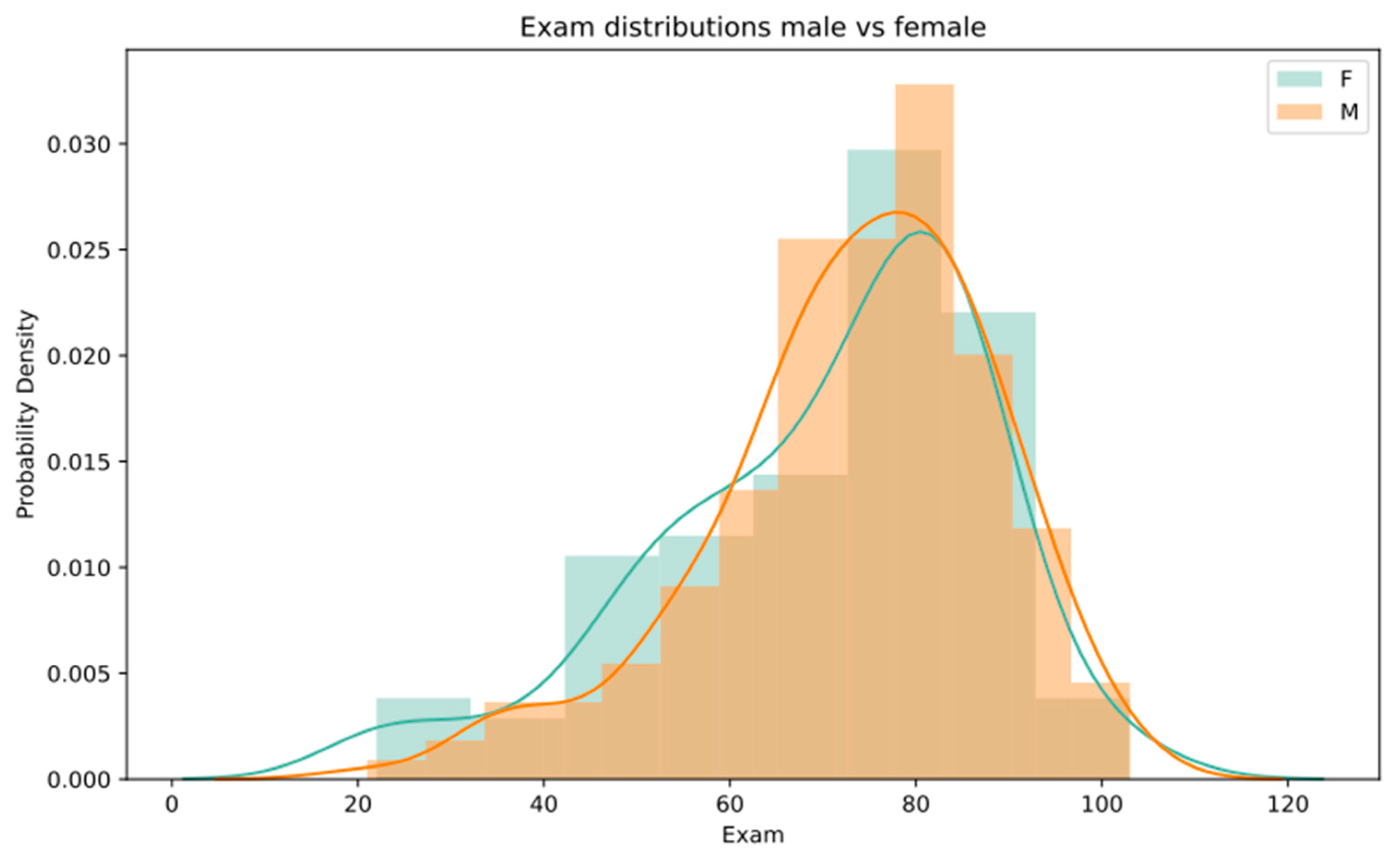
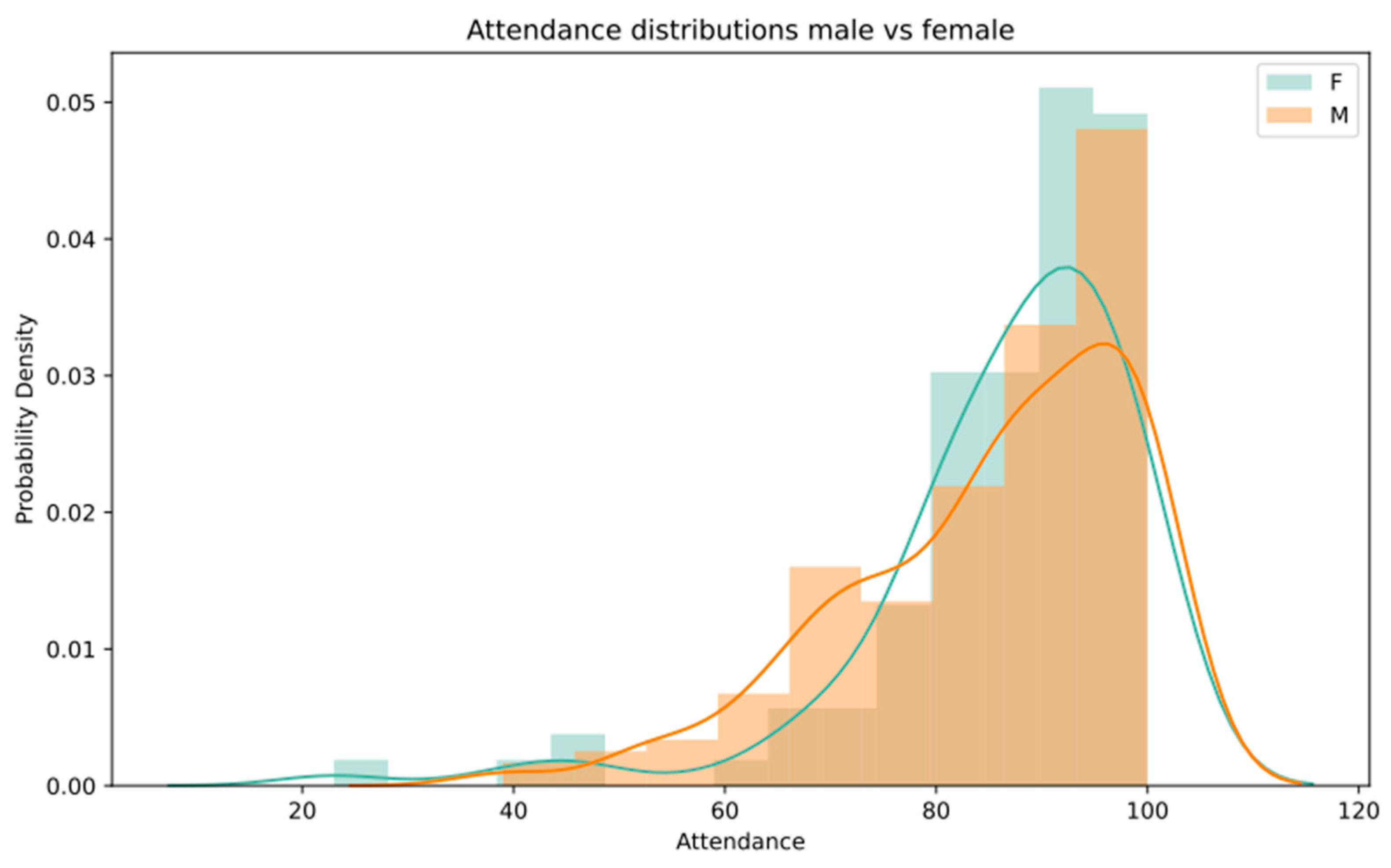
3.2. Step 2. Comparison of the the Full Male And Female Populations, Regarding Exam and Attendance Score

The PDF graphs with normed histograms for both populations regarding exam and attendance scores are represented in Figure 4 and Figure 5.

The graphs in Figure 4 and Figure 5 show very similar curves, without a clear advantage of one population over the other. The graphs for attendance in Figure 5 show more apparent differences than those for the exam. It shows a higher concentration of the female population in the higher attendance, but a higher concentration of male students in the lower attendance, all with a small margin, making it difficult to predict any of the two populations having a better result. This suggests that the different proportions of male and female students do not have a significant influence in the results of each year.

The key numerical results for both populations are arranged in the same way as in Table 2 above and are summarized in

Table 3. Numerical results of “exam” and “attendance” scores of female and male populations.

Parameters	Exam Female	Exam Male	Att. Female	Att. Male
Count	103	175	103	175
Mean	70.23	73.31	86.58	85.29
Std	17.54	15.25	13.21	13.56
Minimum	22.00	21.00	23.00	39.00
25%	59.15	66.00	81.65	77.00
50%	75.00	75.90	90.00	88.00
75%	83.00	84.00	94.15	97.25
Maximum	103.00	103.00	100.00	100.00

.

The Mann–Whitney U test calculation resulted on the following p-values:

• Exam score female vs. male, p = 0.855, the alternative hypothesis cannot be confirmed, and therefore it is not possible to conclude that one group exam score will be better than the other.
• Attendance score female vs. male, p = 0.255 for the alternative hypothesis (female students having better attendance than male students), therefore it is not possible to conclude that one group attendance score will be better than the other.

This step allowed us to discard any significant difference in performance between male and female populations.

Steps 1 and 2 were very clear in demonstrating the positive influence of natural light in the academic performance, when considering the whole populations of the six years. Regarding attendance, even though the score of the windows group was higher than that of the basement group, the Mann–Whitney U test demonstrated that the difference is not significant. Equally, the difference in performance between the whole male and female populations was not significant for either of the two parameters: exam and attendance. This suggests that the lack of natural light affects similarly male and female populations in short term intellectual activities (three hours periods of the classes). On the other hand, the lack of significant differences in the attendance score between windows and basement populations, and between the whole of the male and female populations, suggests that the deprivation of natural light for the same short time intervals does not have apparent negative physical or psychological effects in the long term (16 weeks). At this point of the research, the question was: if we perform the same tests on individual years, will the results be consistent with the ones discussed until now? To find out, the next step focused on testing the possible influence of the different circumstances between individual years.

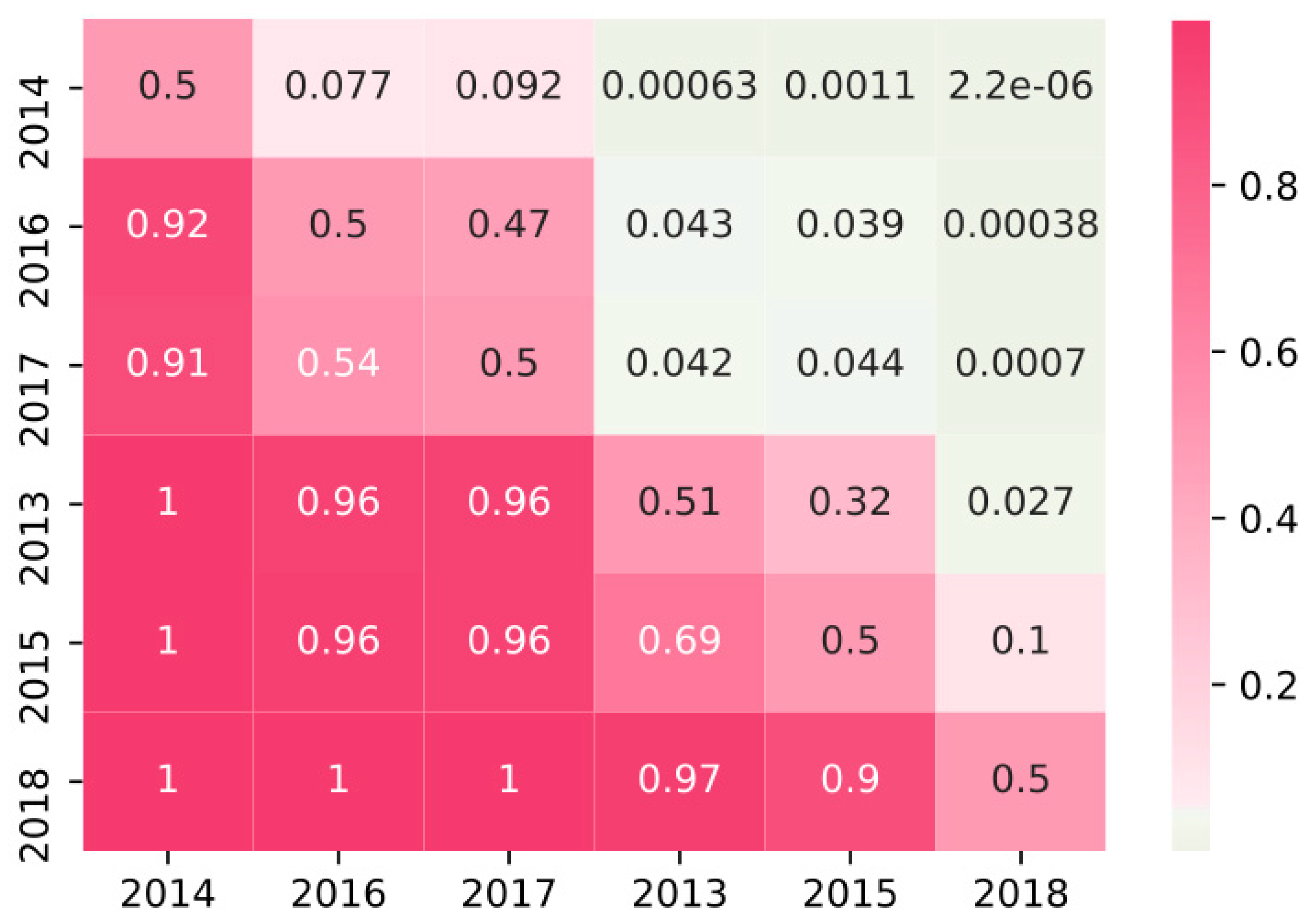
3.3. Step 3. Checking the Possible Influence of Individual Circumstances of Each Year

The boxplot diagrams of (1) the Exam scores by year, with overlap of the number of students per class (2) exam scores by year, separating male and female populations, and (3) attendance scores by year, separating male and female populations, are reproduced below, respectively in Figure 6, Figure 7 and Figure 8.

The boxplots above support the results of the calculations in the previous steps. Figure 6 clearly suggests a better result of exams in the windows classrooms over the six years. However, the variation among similar groups (windows and basement) is also visually noticeable along the years. This fact suggested further testing, which was done in step 4, to quantify the probability of the alternative hypothesis (windows having better exam than basement, considering individual years). The second observation of Figure 6 is that the influence of the size of the classrooms in the results is less conclusive. This suggested the need of further testing to discard the influence of classroom size in the exam results. This was also done in step 4.

Figure 7 and Figure 8 confirmed that the changing ratio of male vs. female students has no visible influence in the results of exam or attendance. Therefore, no further testing was done in this aspect.

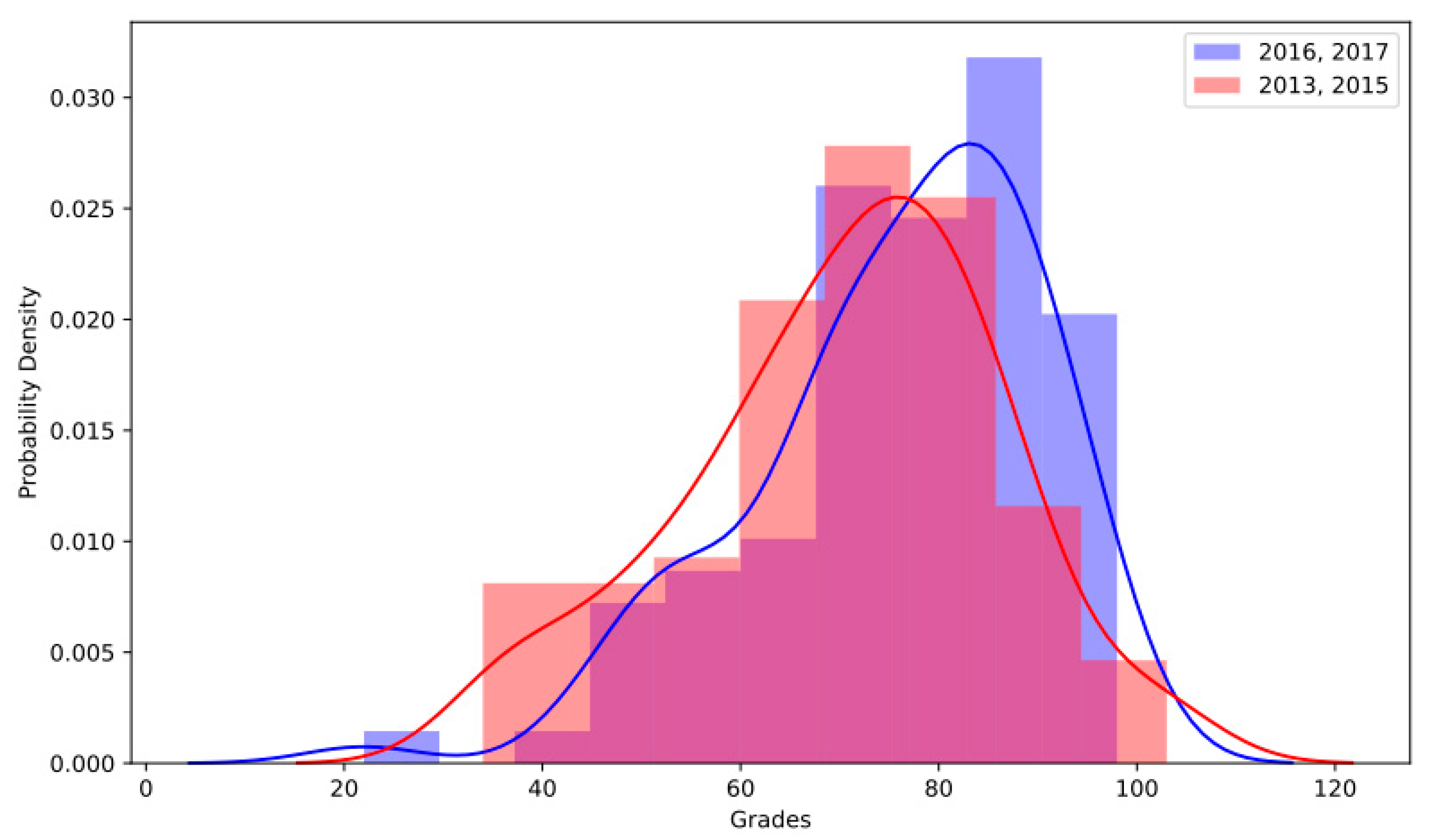
3.4. Step 4. Further Testing by Individual Years, or by Year Groups

The results in the previous steps suggested the need to further test individual years against each other. The Mann–Whitney U test was done each year against every other year, with the results of the p-value for the alternative hypothesis summarized in Figure 9.

The p-values for the alternative hypothesis in the window years (2014, 2016 and 2017) performing better ranges between p = 0.044 in the worst case, to p << 0.001 in the most favorable. This makes a clear distinction between the two populations and confirms the alternative hypothesis for the window years with a confidence level over 95%. One interesting fact to stress at this point is that 2017 was an underground classroom, with clerestory windows, and an interior space very similar to the other basement windows (Figure 1). This allows us to discard the possible effect of an exterior view at eye level windows, as it is not as decisive (again, in short term intellectual activities) as just the fact of having natural light. This observation is consistent with the Heshong Mahone Group reports of 1999 [14,20].

At this point, further testing on the influence of the number of students in each class was done. It seems intuitive that smaller groups produce better academic results. Figure 10 shows a plot of student count related to the exam result.

The graph suggests a tendency to lower exam scores as the count of students increases. However, there are also very similar results between years with significant difference in the count of students (2014 vs. 2017, and 2015 vs. 2013). If we omit the best (2014) and the worst (2018) years, which are very extreme, the trend is not so clear. To check for this trend with some level of confidence, a regression would be necessary, but there are not enough data for it to be reliable. Instead, a new test was done with the whole population of “windows” vs. “basement”, excluding the two extreme years, in order to discard possible distortions due to their exceptionality. Figure 11 shows the PDF graph with normed histograms of the exam score for the accumulated populations of “windows” (2016, 2017) and “basement” (2013, 2015).

Figure 11, even when not as rotund as Figure 2, shows a very clear difference of distribution for both populations, suggesting the results in the exam result will be significantly better for windows.

In this new calculation, key numerical results for both populations, including count, mean value (Mean), standard deviation (Std), minimum, 25%, 50% and 75% quartiles, and maximum, are summarized in

Table 4. Numerical results of “exam” scores of “basement” and “windows” populations, excluding the extreme years of 2014 and 2018.

Parameters	Exam Windows	Exam Basement
Count	91	100
Mean	75.81	70.37
Std	14.56	15.74
Minimum	22.00	34.00
25%	68.00	61.03
50%	78.00	73.40
75%	86.00	81.18
Maximum	98.00	103.00

.

The Mann–Whitney U test calculation resulted in p = 0.007, confirming the alternative hypothesis: windows classroom exam scores will be better than those of the basement classroom, with a confidence level of 99.3%. The results are consistent with the ones derived from the whole populations in step 1. Furthermore, the p-value is also extremely small, allowing for a rotund rejection of the null hypothesis, and confirming that in all cases, the windows classrooms will perform better than the basement ones.

3.5. Summary

The most important results of the whole calculation process are summarized in

Table 5. Results summary. W stands for “windows”. B stands for “basement”. M stands for “male students”. F stands for “female students”. H1 stands for “alternative hypothesis” in the Mann Whitney U test. Att stands for “attendance”. Y stands for “year”.

Populations Tested	H1	Mean Values	p-Value	Result
All W vs. B	Exam W > B	77.19(W); 68.21(B)	p << 0.001	true
All W vs. B	Att W > B	86.93(W); 84.85(B)	p = 0.143	false
All F vs. M	Exam F > M	70.23(F); 73.31(M)	p = 0.855	false
All F vs. M	Att F > M	86.58(F); 85.29(M)	p = 0.255	false
Every Y vs. every other Y	Exam WY > BY	--	p = 0.044 to p << 0.001	true
W vs. B except extreme Y	Exam W > B	75.81(W); 70.37(B)	p = 0.007	true

.

4. Conclusions

This is a case study performed over existing academic data, with the advantage of the data being objective and taken from real life activity (as opposed to subjective Likert scale surveys or experiments based on simulations), with a sample population large enough to draw significant conclusions. Notwithstanding the limitations, the present case study adds new data to the reviewed literature in the field, in different geographical and academic contexts.

The experiment was done over a population of a total of 278 university students accumulated during six consecutive courses, one per year. The courses consisted of three-hour theoretical lectures taught once a week, during a span of 16 consecutive weeks. In three of these years, the classrooms had windows, mixing natural and artificial light. In the other three, the classrooms were underground, with only artificial light, consisting in FSFL. The research was done over objective data on the students’ performance, primarily, the exam score, and secondarily, attendance. The results provided strong evidence on the negative effect of the deprivation of natural light in short term intellectual ability. After testing the results to discard the influence of other factors, such as number of students per class or differences on the ratio of male and female students, classroom with windows performed consistently better in the exams. For the whole population of windows vs. basement classrooms, the difference in the mean exam score was 13.13% better, while the Mann–Whitney U test was conclusive on the prevision of windows classrooms having better exam scores than the basement classrooms with a p-value of p << 0.001. Even excluding the most extreme years (best and worse) from the calculations, the mean score was still a noticeable 7.73% better. In this case, the p-value was also a rotund p = 0.007. These results are consistent with previous research [17,20]. The present case demonstrates that the effect is felt in short periods of time, even in a population to which a high motivation and high intellectual level is presupposed. These results agree with the existing literature, stressing the need of regulations and architectural design standards to care not only for quantitative aspects of lighting (as the illuminance), but also about the quality of the natural light used in these spaces [7]. Even in short term occasional use, if a critical activity requiring intellectual performance is happening (court rooms, surgery theatres, classrooms, etc.), the inclusion of natural light should be seriously considered whenever possible. On the other hand, no apparent negative effect was suggested in the long term, as the other parameter studied, attendance, did not show significant differences between both groups.

As for future research steps, the present experiment will not have continuity, as in 2019, the methodology was updated, and from 2020, the course is advised to be performed always in classrooms with natural light. It would be interesting to test the results of similar courses taught during day and night time, where there is no choice on the lighting system. Additional research could test how newly developing and expanding LED technologies perform against natural light and traditional FSFL.

References

1. Robinson, W. The 1962 Sir Alfred Herbert paper: Lighting and the production engineer. Prod. Eng. 1963, 42, 123–139. [Google Scholar] [CrossRef]
2. Boubekri, M. Daylighting Design: Planning Strategies and Best Practice Solutions; Birkhäuser: Basel, Switzerland, 2014. [Google Scholar]
3. Webb, A.R. Considerations for lighting in the built environment: Non-visual effects of light. Energy Build. 2006, 38, 721–727. [Google Scholar] [CrossRef]
4. Boyce, P.R. Review: The impact of light in buildings on human health. Indoor Built Environ. 2010, 19, 8–20. [Google Scholar] [CrossRef]
5. USBGC. Daylight Credits in LEED v4.1. 2018. Available online: https://www.usgbc.org/credits/new-construction-schools-new-construction-retail-new-construction-data-centers-new-constru-4 (accessed on 20 April 2020).
6. Hua, Y.; Oswald, A.; Yang, X. Effectiveness of daylighting design and occupant visual satisfaction in a leed gold laboratory building. Build. Environ. 2011, 46, 54–64. [Google Scholar] [CrossRef]
7. Kralikova, R.; Piňosová, M.; Hricová, B. Lighting quality and its effects on productivity and human healts. Int. J. Interdiscip. Theory Pract. 2016, 10, 8–12. [Google Scholar]
8. Altomonte, S. Ch2-lighting and physiology. Constr. Econ. Build. 2005, 5, 40–46. [Google Scholar] [CrossRef] [Green Version]
9. Galasiu, A.D.; Veitch, J.A. Occupant preferences and satisfaction with the luminous environment and control systems in daylit offices: A literature review. Energy Build. 2006, 38, 728–742. [Google Scholar] [CrossRef] [Green Version]
10. Gou, Z.; Lau, S.S.-Y.; Shen, J. Indoor environmental satisfaction in two leed offices and its implications in green interior design. Indoor Built Environ. 2012, 21, 503–514. [Google Scholar] [CrossRef]
11. Buffoli, M.; Capolongo, S.; Cattaneo, M.; Signorelli, C. Project, natural lighting and comfort indoor. Ann. Ig. 2007, 19, 429–441. [Google Scholar] [PubMed]
12. Kamali, N.J.; Abbas, M.Y. Healing environment: Enhancing nurses’ performance through proper lighting design. Procedia Soc. Behav. Sci. 2012, 35, 205–212. [Google Scholar] [CrossRef] [Green Version]
13. Quartier, K.; Vanrie, J.; Van Cleempoel, K. As real as it gets: What role does lighting have on consumer’s perception of atmosphere, emotions and behaviour? J. Environ. Psychol. 2014, 39, 32–39. [Google Scholar] [CrossRef]
14. Heshong Mahone Group. Skylighting and Retail Sales. An Investigation Into the Relationship between Daylighting and Human Performance; Pacific Gas and Electric Company: Fair Oaks, CA, USA, 1999. [Google Scholar]
15. Larson, C.T. The Effect of Windowless Classrooms on Elementary School Children. 1965. Available online: https://eric.ed.gov/?id=ED014847 (accessed on 20 April 2020).
16. Hathaway, W.E. A Study Into the Effects of Light on Children of Elementary School-Age--A Case of Daylight Robbery; Policy and Plaiming Branch, Planning and Information Services Division, Alberta Education: Alberta, AB, Canada, 1992.
17. Nicklas, M.H.; Bailey, G.B. Analysis of the Performance of Students in Daylit Schools. Available online: https://eric.ed.gov/?id=ED458782 (accessed on 19 May 2020).
18. McColl, S.L.; Veitch, J.A. Full-spectrum fluorescent lighting: A review of its effects on physiology and health. Psychol. Med. 2001, 31, 949–964. [Google Scholar] [CrossRef] [PubMed]
19. Pulay, A.; Williamson, A. A case study comparing the influence of led and fluorescent lighting on early childhood student engagement in a classroom setting. Learn. Environ. Res. 2019, 22, 13–24. [Google Scholar] [CrossRef]
20. Heshong Mahone Group. Daylighting in Schools an Investigation Into the Relationship between Daylighting and Human Performance; Pacific Gas and Electric Company, California Board for Energy Efficiency: Fair Oaks, CA, USA, 1999. [Google Scholar]
21. Korea University. Homepage of the Department of Architecture. Available online: https://doa.korea.edu (accessed on 17 May 2020).
22. Korea University. Bachelor of Architecture Curriculum. Available online: https://doa.korea.edu/archi_en/matriculate/curriculum.do (accessed on 17 May 2020).
23. PHILLIPS. Simply Energy Saving, Master TL-d Eco. 2020. Available online: https://www.assets.signify.com/is/content/PhilipsLighting/comf2538-pss-global (accessed on 17 May 2020).
24. Forbes, C.; Evans, M.; Hastings, N.; Peacock, B. Statistical Distributions; John Wiley & Sons: Hoboken, NJ, USA, 2011. [Google Scholar]
25. Hastie, T.; Tibshirani, R.; Friedman, J. The Elements of Statistical Learning: Data Mining, Inference, and Prediction; Springer Science & Business Media: Berlin, Germany, 2009. [Google Scholar]
26. Mann, H.B.; Whitney, D.R. On a test of whether one of two random variables is stochastically larger than the other. Ann. Math. Stat. 1947, 18, 50–60. [Google Scholar] [CrossRef]
27. Tukey, J.W. Box-and-Whisker Plots. In Exploratory Data Analysis; Pearson: London, UK, 1977; pp. 39–43. ISBN 978-0201076165. [Google Scholar]
28. Python Software Foundation, Python Programming Language. Available online: https://www.python.org/ (accessed on 19 April 2020).
29. Scipy-Developers. Scipy Library. Available online: https://www.scipy.org/scipylib/index.Html (accessed on 19 April 2020).
30. The Pandas Development Team, Pandas. Available online: https://pandas.pydata.org/ (accessed on 19 April 2020).
31. Waskom, M. Seaborn: Statistical Data Visualization. Available online: https://seaborn.pydata.org/index.Html (accessed on 19 April 2020).
Figure 1. Photos of the interior space of each type of classroom: (a) Basement (2013, 2015 and 2018); (b) Windows (2014 and 2016); (c) Clerestory windows with no exterior view (2017).
Sustainability 12 04167 g001
Figure 2. PDF graph with normed histograms of the exam score of the two populations, “windows” (blue) vs. “basement” (red).
Sustainability 12 04167 g002
Figure 3. PDF graph with normed histograms of the attendance score of the two populations, “windows” (blue) vs. “basement” (red).
Sustainability 12 04167 g003
Figure 4. PDF graph with normed histograms overlap of the exam score of the two populations, female (green) vs. male (orange).
Sustainability 12 04167 g004
Figure 5. PDF graph with normed histograms overlap of the attendance score of the two populations, female (green) vs. male (orange).
Sustainability 12 04167 g005
Figure 6. Boxplot of the exam score (values in the left vertical axis) of the two populations, “windows” (blue) vs. “basement” (red), by years, and with overlap of the number of students (histograms in light blue, with values in the right vertical axis).
Sustainability 12 04167 g006
Figure 7. Boxplot of the exam score of the two populations, female (green) vs. male (orange), by years.
Sustainability 12 04167 g007
Figure 8. Boxplot of the attendance score of the two populations, female (green) vs. male (orange), by years.
Sustainability 12 04167 g008
Figure 9. Heatmap diagram of the Mann–Whitney U Test p-values, comparing all individual years for the alternative hypothesis: the years in the rows (left) will be better than the years in the columns (below). The green color means rejection of the null hypothesis and the pink color means no rejection of the null hypothesis. Years 2014, 2016 and 2017 above and on the left, are “windows”, the other “basement”.
Sustainability 12 04167 g009
Figure 10. Plot graph of student count (horizontal axis) and exam score median (vertical axis). In blue are “windows” years, and in red are “basement” years.
Sustainability 12 04167 g010
Figure 11. PDF graph with normed histogram of the exam score of the two populations, excluding the extreme years of 2014 and 2018, “windows” (blue) vs. “basement” (red).
Sustainability 12 04167 g011