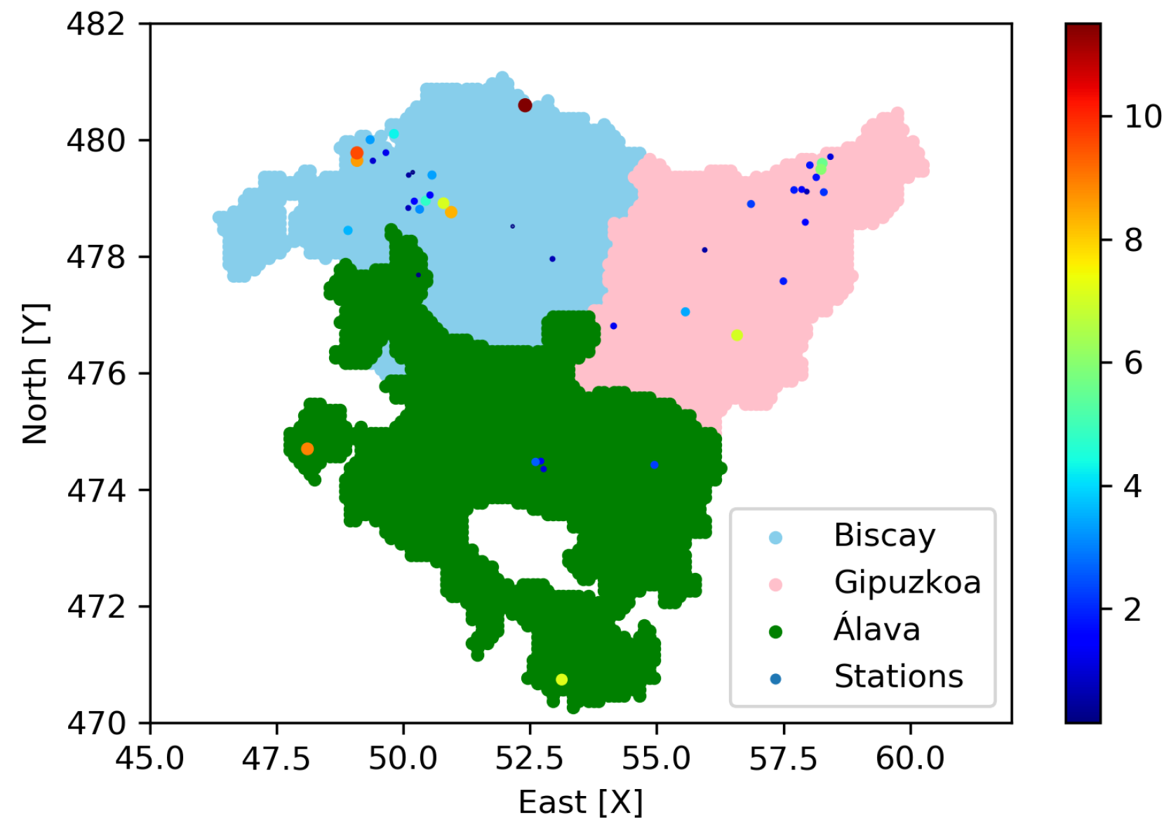
Figure 1.
Location of the monitoring stations.
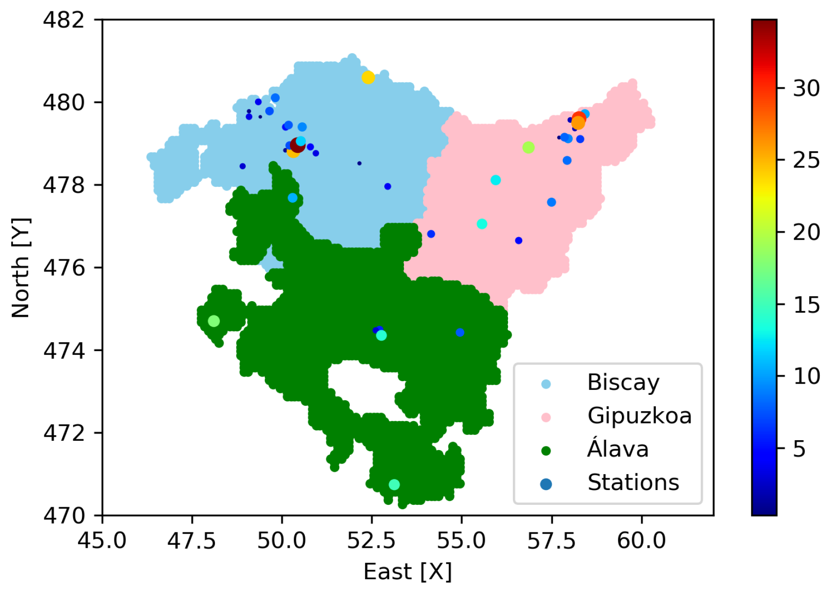
Figure 1.
Location of the monitoring stations.
Figure 2.
Sequence of the main stages of the study.
Figure 2.
Sequence of the main stages of the study.
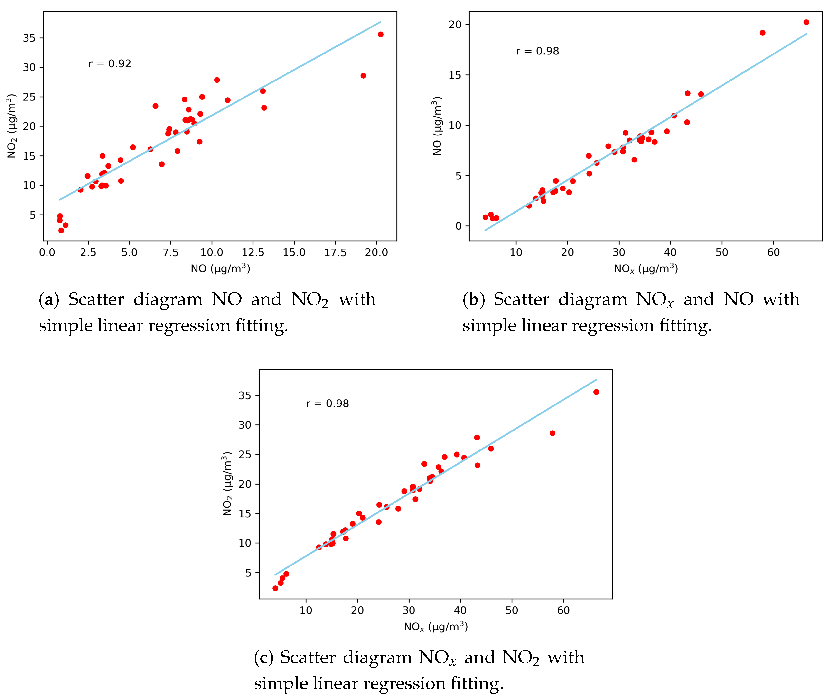
Figure 3.
Scatter diagrams using simple linear regression.
Figure 3.
Scatter diagrams using simple linear regression.
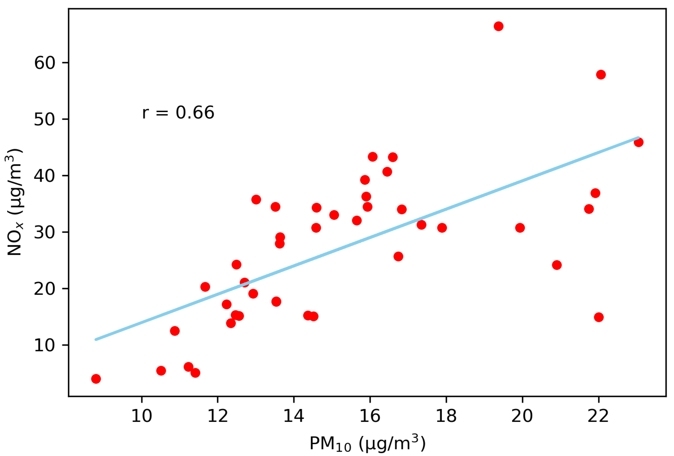
Figure 4.
Scatter diagram PM and NO with simple linear regression fitting.
Figure 4.
Scatter diagram PM and NO with simple linear regression fitting.
Figure 5.
Scatter diagram NO obtained by MLR and NO sampled in monitoring stations.
Figure 5.
Scatter diagram NO obtained by MLR and NO sampled in monitoring stations.
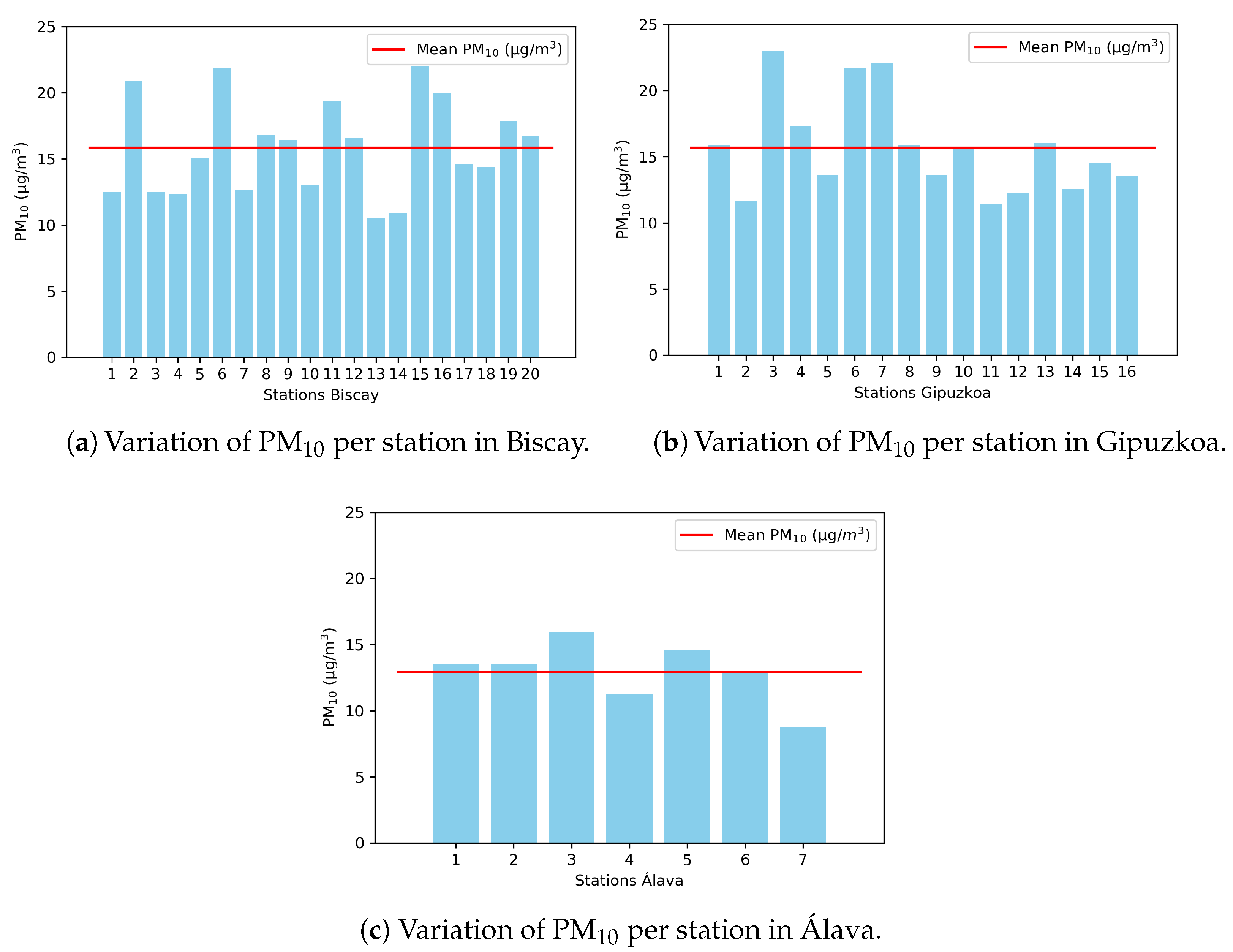
Figure 6.
Variation of PM per station.
Figure 6.
Variation of PM per station.
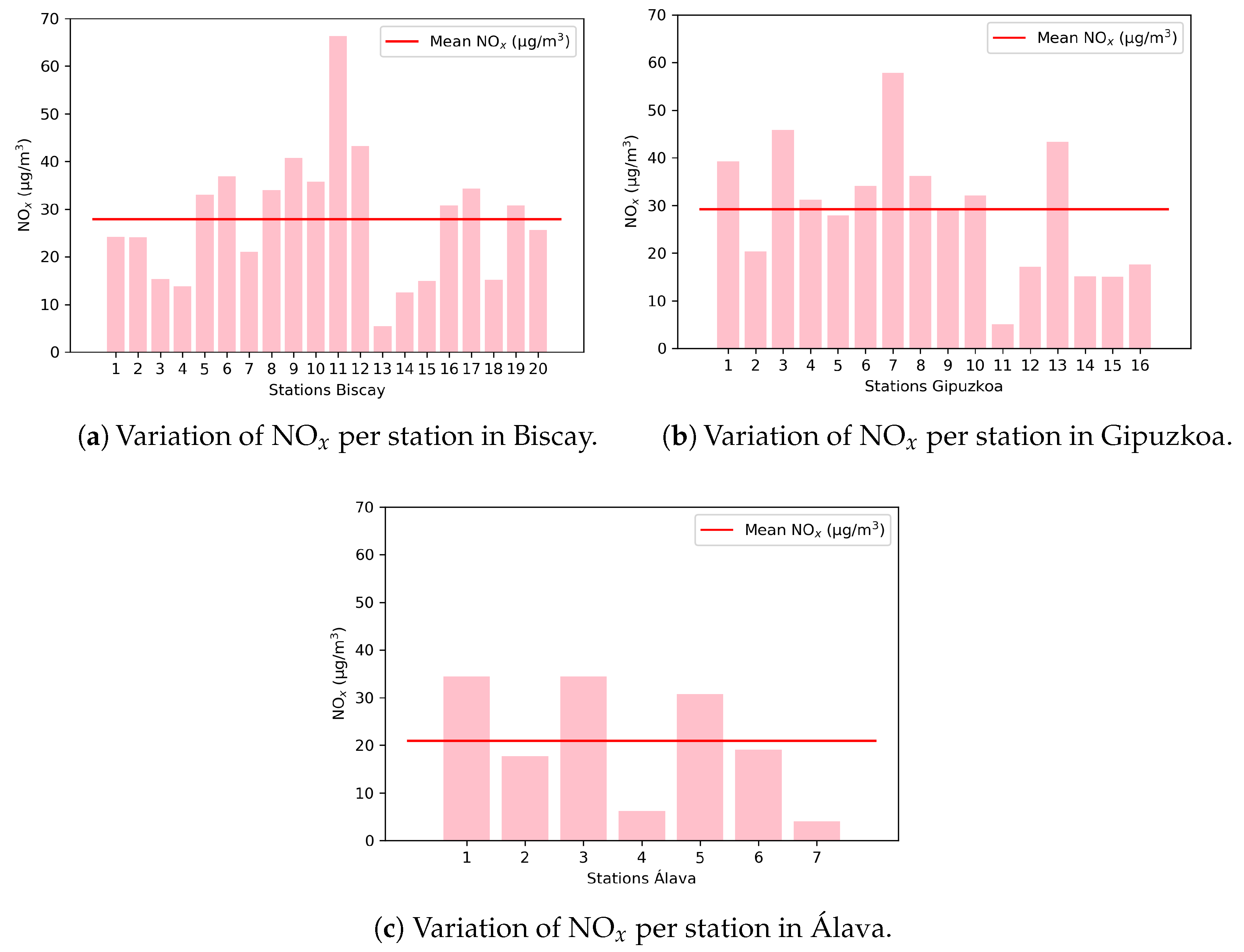
Figure 7.
Variation of NO per station.
Figure 7.
Variation of NO per station.
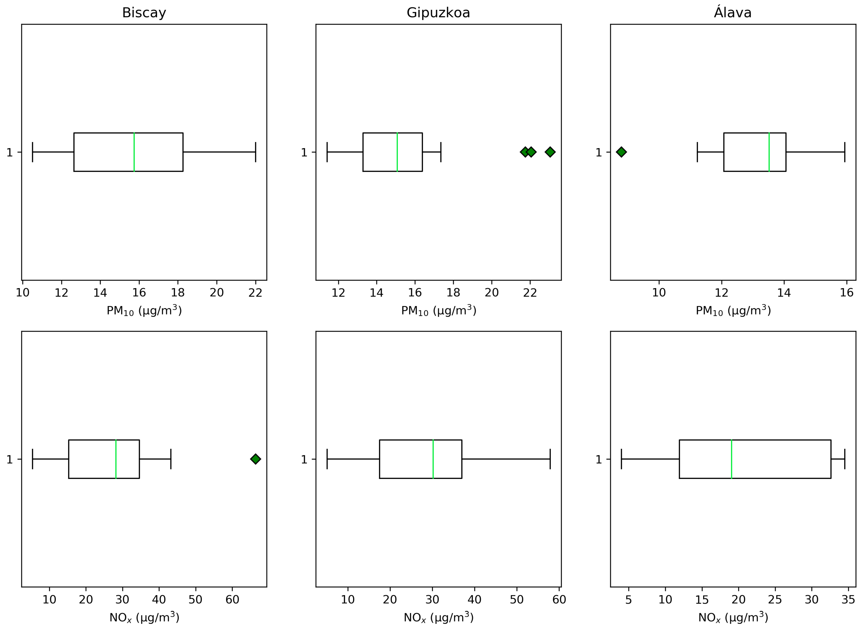
Figure 8.
Anomalous values in each province for each pollutant (PM and NO).
Figure 8.
Anomalous values in each province for each pollutant (PM and NO).
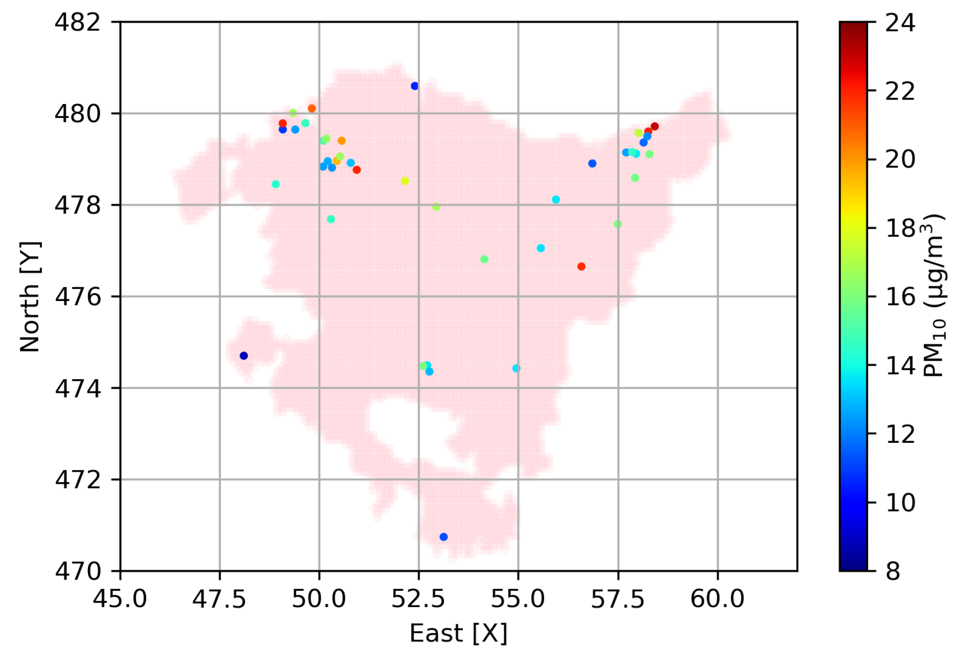
Figure 9.
PM measurements per monitoring station (in 10,000 m both axes).
Figure 9.
PM measurements per monitoring station (in 10,000 m both axes).
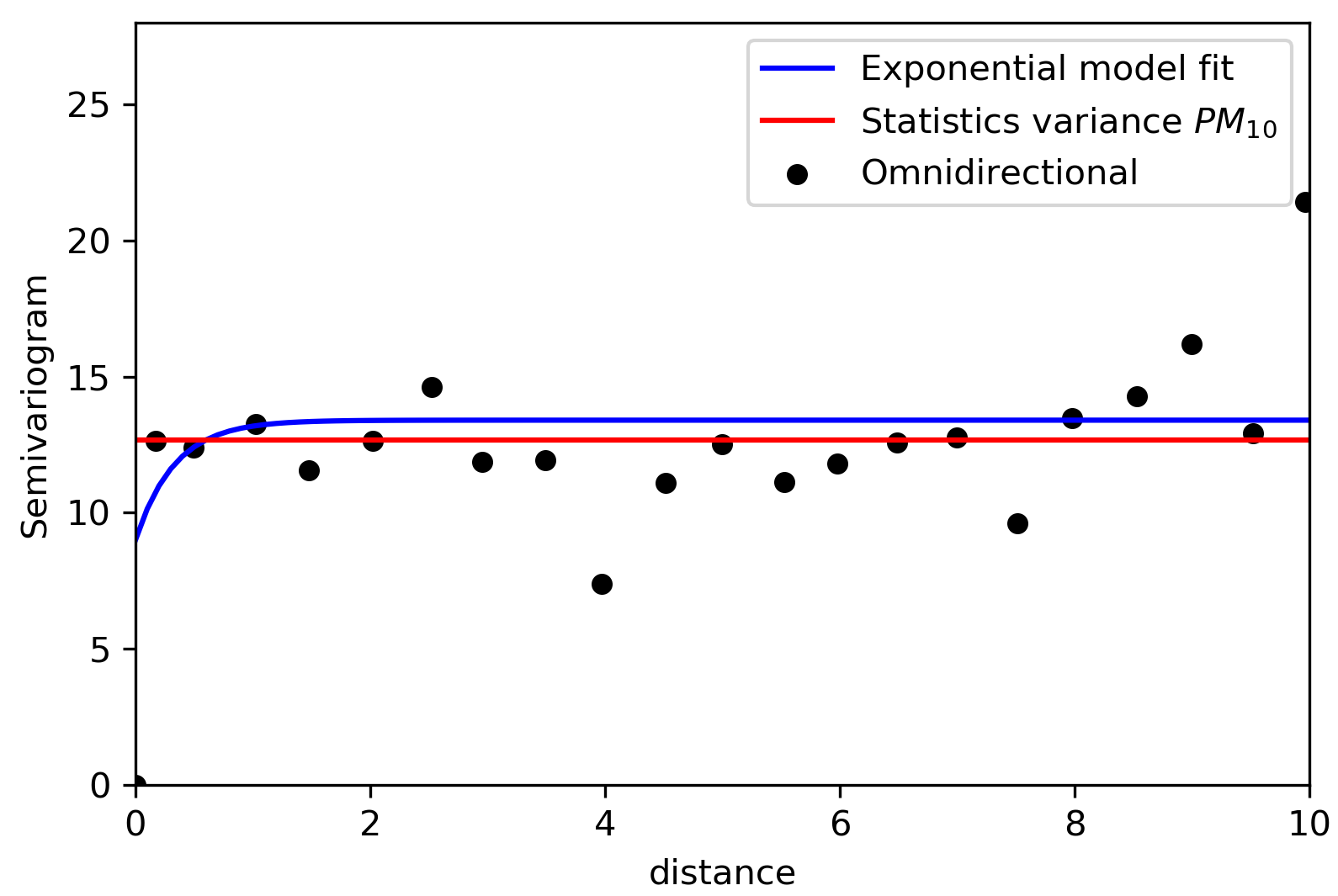
Figure 10.
Experimental semivariogram of PM in the Basque Country (in 10,000 m the horizontal axis).
Figure 10.
Experimental semivariogram of PM in the Basque Country (in 10,000 m the horizontal axis).
Figure 11.
Fit nested structural model of PM in each province (in 10,000 m the horizontal axis).
Figure 11.
Fit nested structural model of PM in each province (in 10,000 m the horizontal axis).
Figure 12.
Fit nested structural model of PM in the Basque Country (in 10,000 m the horizontal axis).
Figure 12.
Fit nested structural model of PM in the Basque Country (in 10,000 m the horizontal axis).
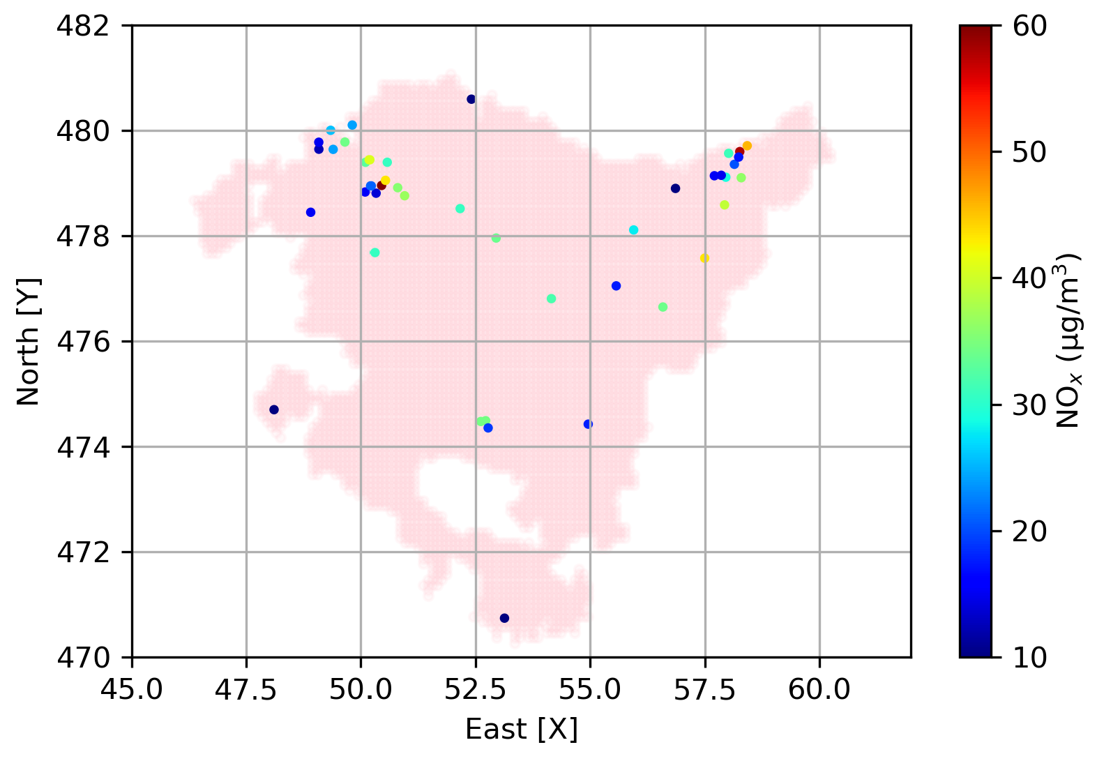
Figure 13.
NO measurements per monitoring station (in 10,000 m in both axes).
Figure 13.
NO measurements per monitoring station (in 10,000 m in both axes).
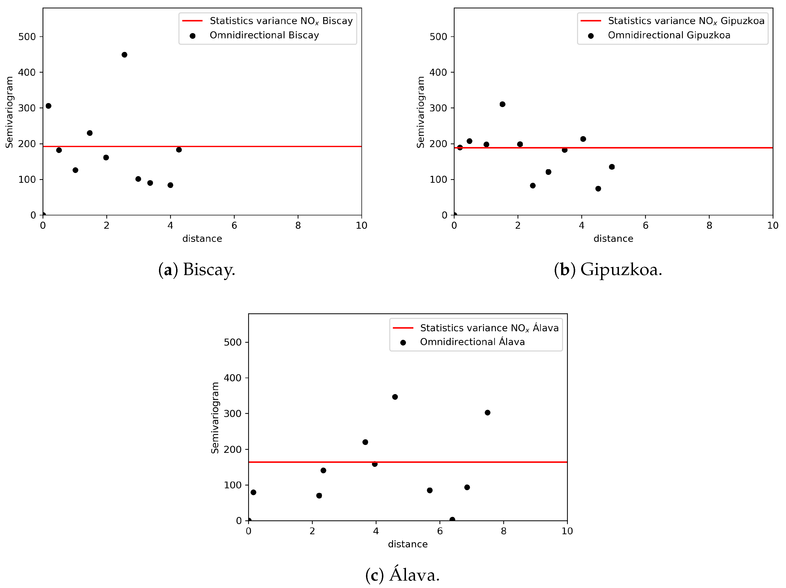
Figure 14.
Experimental semivariogram of NO in each province (in 10,000 m the horizontal axis).
Figure 14.
Experimental semivariogram of NO in each province (in 10,000 m the horizontal axis).
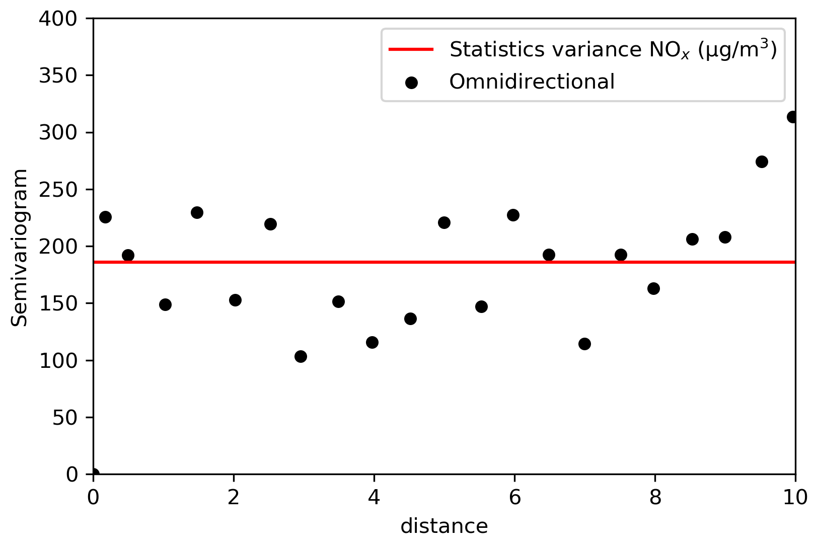
Figure 15.
Experimental semivariogram and pure nugget effect model of NO in the Basque Country (in 10,000 m the horizontal axis).
Figure 15.
Experimental semivariogram and pure nugget effect model of NO in the Basque Country (in 10,000 m the horizontal axis).
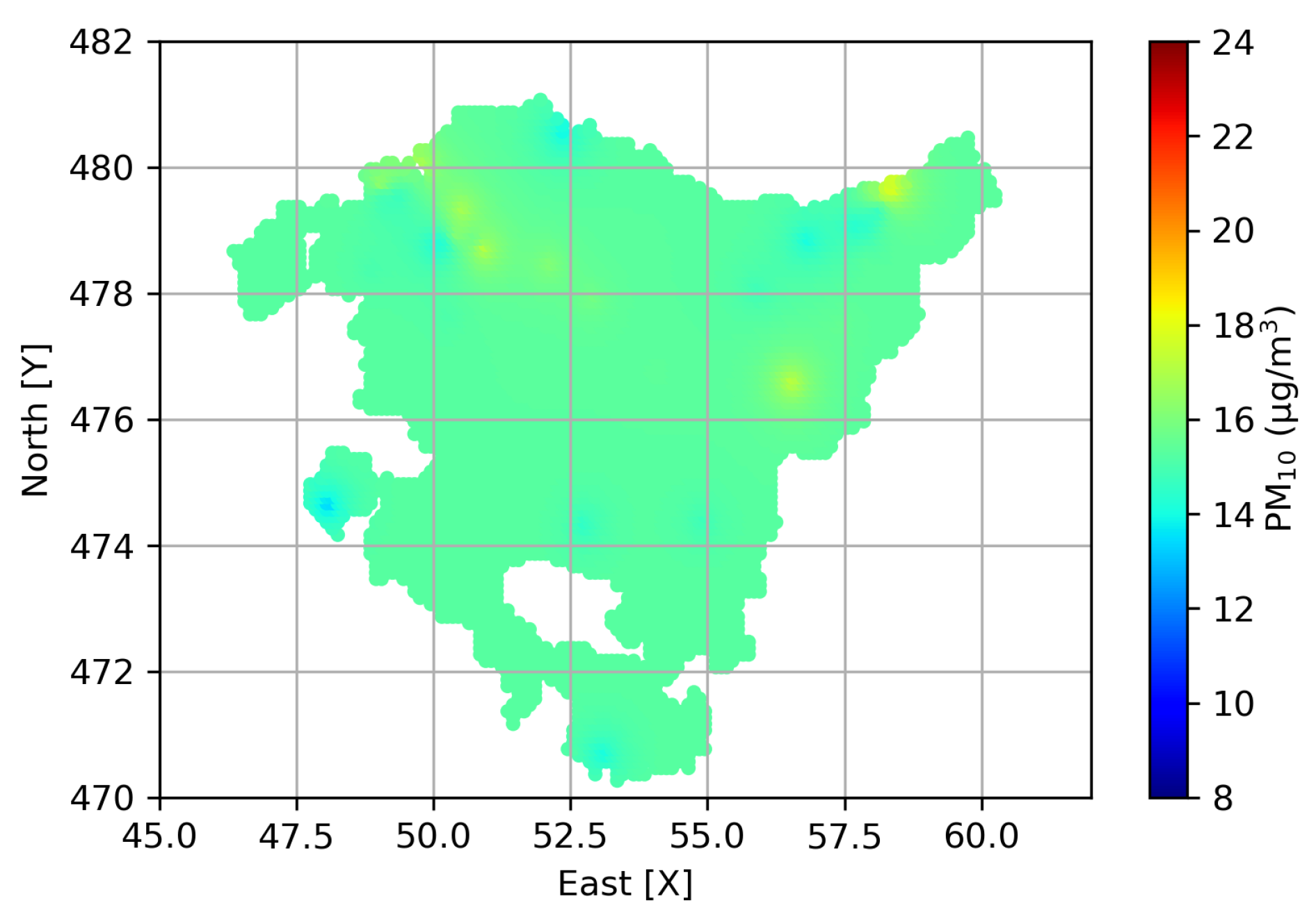
Figure 16.
PM map in the Basque Country generated by simple kriging (in 10,000 m both axes).
Figure 16.
PM map in the Basque Country generated by simple kriging (in 10,000 m both axes).
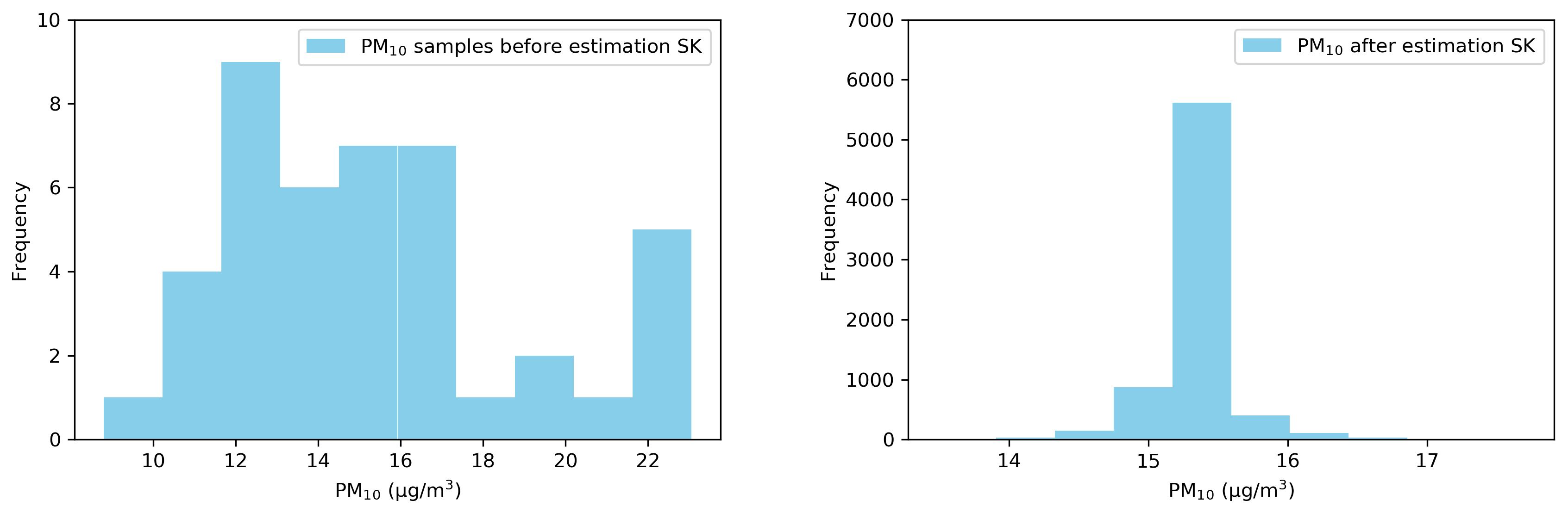
Figure 17.
Histograms of PM before (left) and after (right) simple kriging application.
Figure 17.
Histograms of PM before (left) and after (right) simple kriging application.
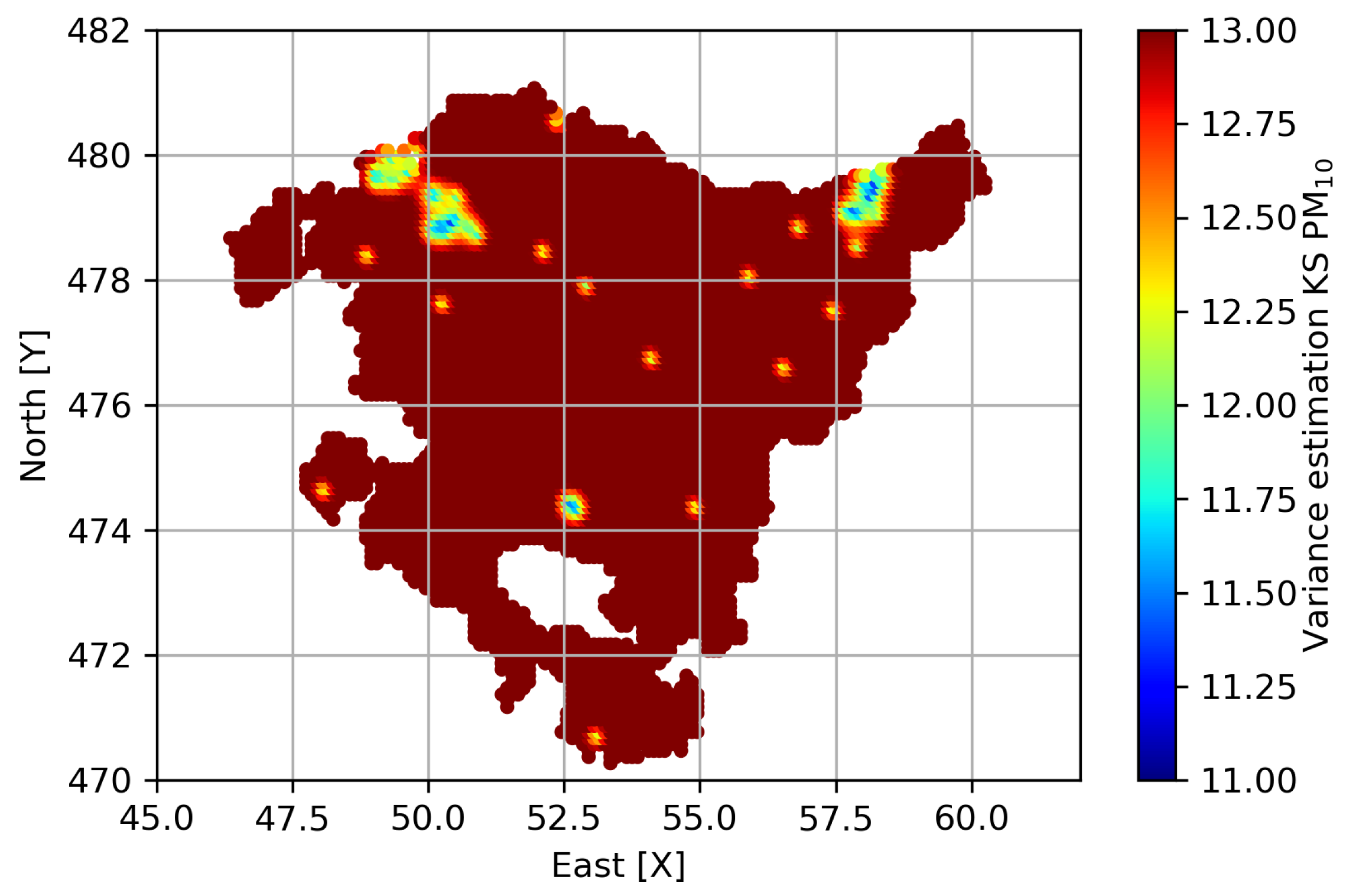
Figure 18.
Map of the PM variance ((PM)) in the Basque Country generated by simple kriging (in 10,000 m both axes).
Figure 18.
Map of the PM variance ((PM)) in the Basque Country generated by simple kriging (in 10,000 m both axes).
Figure 19.
PM map in the Basque Country generated by linear-type RBF (in 10,000 m both axes).
Figure 19.
PM map in the Basque Country generated by linear-type RBF (in 10,000 m both axes).
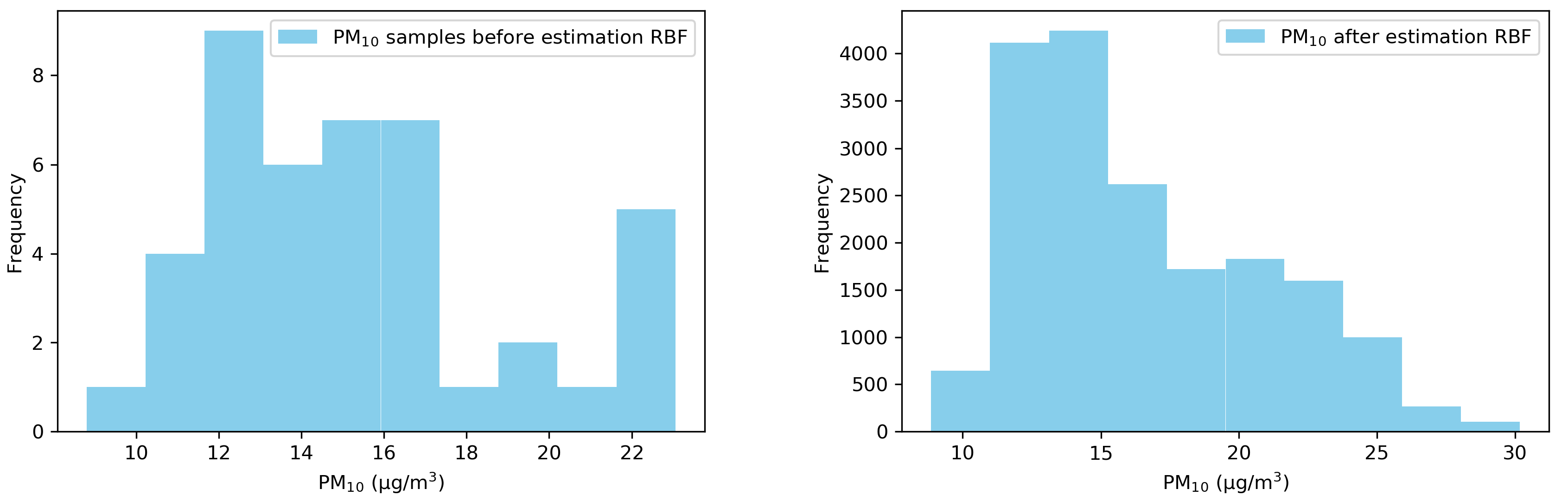
Figure 20.
Histograms of PM before (left) and after (right) linear-type RBF application.
Figure 20.
Histograms of PM before (left) and after (right) linear-type RBF application.
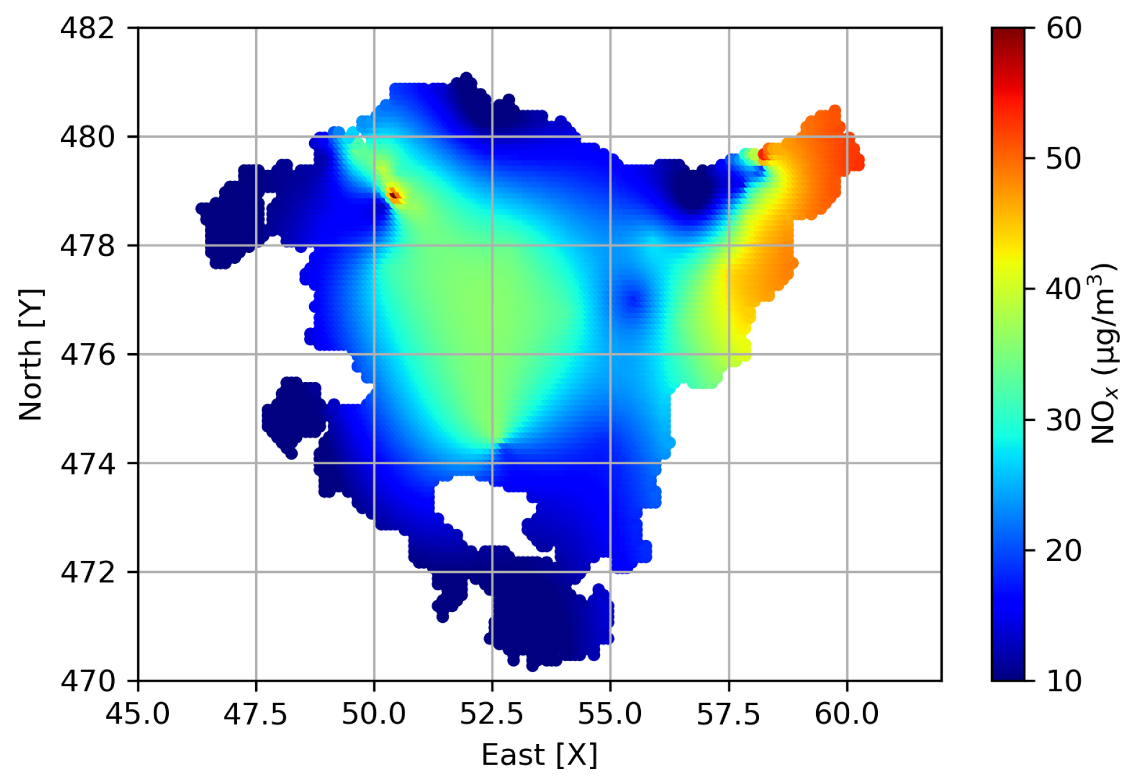
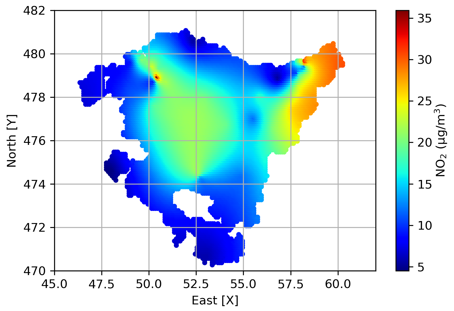
Figure 21.
NO map in the Basque Country generated by linear-type RBF (in 10,000 m in both axes).
Figure 21.
NO map in the Basque Country generated by linear-type RBF (in 10,000 m in both axes).
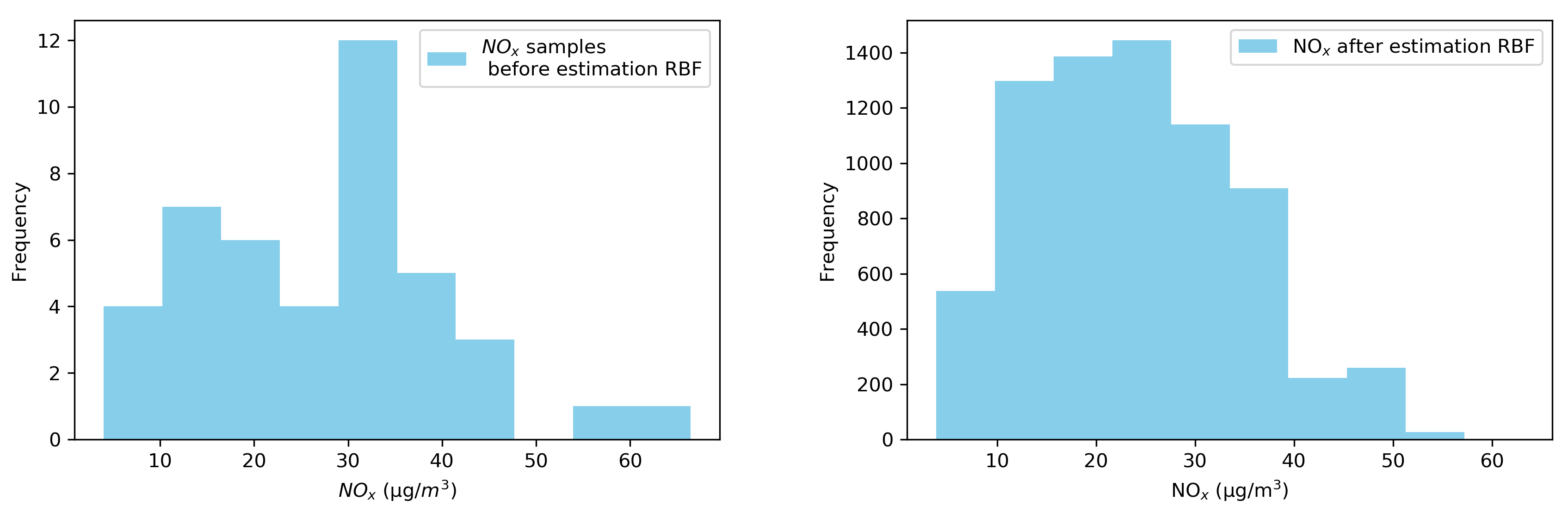
Figure 22.
Histograms of NO before (left) and after (right) linear-type RBF application.
Figure 22.
Histograms of NO before (left) and after (right) linear-type RBF application.
Figure 23.
Absolute error in PM per station (in 10,000 m in both axes).
Figure 23.
Absolute error in PM per station (in 10,000 m in both axes).
Figure 24.
Absolute error in NO per station (in 10,000 m in both axes).
Figure 24.
Absolute error in NO per station (in 10,000 m in both axes).
Figure 25.
NO map in the Basque Country generated by using the simple linear regression model from NO (in 10,000 m in both axes).
Figure 25.
NO map in the Basque Country generated by using the simple linear regression model from NO (in 10,000 m in both axes).
Figure 26.
NO map in the Basque Country generated by using the simple linear regression model from NO (in 10,000 m in both axes).
Figure 26.
NO map in the Basque Country generated by using the simple linear regression model from NO (in 10,000 m in both axes).
Table 1.
Limits for NO and PM established by RD 102/2011.
Table 1.
Limits for NO and PM established by RD 102/2011.
| Pollutant | Average | Limit Value | Alarm Threshold | Compliance Date |
|---|
| NO | Hourly | 200 g/m | 400 μg/m3 (during 3 h) | 1 January 2010 |
| | | (18 greater values maximum per year) | | |
| | Annual | 40 μg/m3 | | 1 January 2010 |
| PM | Daily | 50 g/m | 400 μg/m3 (during 3 h) | 1 January 2005 |
| | | (35 greater values maximum per year) | | |
| | Annual | 40 g/m | | 1 January 2005 |
Table 2.
Descriptive statistics of pollutants in Biscay.
Table 2.
Descriptive statistics of pollutants in Biscay.
| Pollutant | Count | Mean | SD | Min. | Q1 | Q2 | Q3 | Max. |
|---|
| NO (μg/m3) | 20 | 6.73 | 4.30 | 0.75 | 3.32 | 6.77 | 8.42 | 20.25 |
| NO (μg/m3) | 20 | 17.71 | 7.66 | 4.04 | 11.17 | 17.72 | 23.00 | 35.59 |
| NO (μg/m3) | 20 | 27.90 | 13.87 | 5.42 | 15.28 | 28.19 | 34.66 | 66.40 |
| PM10 (μg/m3) | 20 | 15.85 | 3.60 | 10.51 | 12.65 | 15.75 | 18.26 | 22.01 |
Table 3.
Descriptive statistics of pollutants in Gipuzkoa.
Table 3.
Descriptive statistics of pollutants in Gipuzkoa.
| Pollutant | Count | Mean | SD | Min. | Q1 | Q2 | Q3 | Max. |
|---|
| NO (μg/m3) | 16 | 7.74 | 4.76 | 1.11 | 3.44 | 8.20 | 9.32 | 19.20 |
| NO (μg/m3) | 16 | 17.47 | 6.80 | 3.24 | 12.11 | 18.10 | 22.39 | 28.61 |
| NO (μg/m3) | 16 | 29.21 | 13.73 | 5.09 | 17.51 | 30.17 | 37.02 | 57.88 |
| PM (μg/m3) | 16 | 15.68 | 3.70 | 11.41 | 13.29 | 15.08 | 16.38 | 23.05 |
Table 4.
Descriptive statistics of pollutants in Álava.
Table 4.
Descriptive statistics of pollutants in Álava.
| Pollutant | Count | Mean | SD | Min. | Q1 | Q2 | Q3 | Max. |
|---|
| NO (μg/m3) | 7 | 4.96 | 3.44 | 0.77 | 2.28 | 4.48 | 8.05 | 8.78 |
| NO (μg/m3) | 7 | 13.29 | 7.77 | 2.36 | 7.77 | 13.28 | 20.32 | 21.25 |
| NO (μg/m3) | 7 | 20.95 | 12.79 | 4.03 | 11.93 | 19.05 | 32.62 | 34.49 |
| PM (μg/m3) | 7 | 12.93 | 2.33 | 8.80 | 12.08 | 13.52 | 14.06 | 15.94 |
Table 5.
Descriptive statistics of pollutants in the Basque Country.
Table 5.
Descriptive statistics of pollutants in the Basque Country.
| Pollutant | Count | Mean | SD | Min. | Q1 | Q2 | Q3 | Max. |
|---|
| NO (μg/m3) | 43 | 6.82 | 4.36 | 0.75 | 3.34 | 7.35 | 8.75 | 20.25 |
| NO (μg/m3) | 43 | 16.90 | 7.37 | 2.36 | 11.16 | 17.40 | 21.69 | 35.59 |
| NO (μg/m3) | 43 | 27.26 | 13.64 | 4.03 | 16.25 | 29.10 | 34.48 | 66.40 |
| PM (μg/m3) | 43 | 15.31 | 3.56 | 8.80 | 12.63 | 14.58 | 16.79 | 23.05 |
Table 6.
Parameters to create the area of study.
Table 6.
Parameters to create the area of study.
| Parameter | Value | Unit of Measurement |
|---|
| X coordinate in the origin | 459,500 | meters (m) |
| Y coordinate in the origin | 4,697,700 | meters (m) |
| Cell width in X | 1000 | meters (m) |
| Cell width in Y | 1000 | meters (m) |
| Number of cells in X | 145 | unities |
| Number of cells in Y | 125 | unities |
| Total number of cells | 18,125 | unities |
Table 7.
Parameters and results of simple krigging.
Table 7.
Parameters and results of simple krigging.
| Parameter | Value |
|---|
| Influence ratio | 6 |
| Minimmum number of samples | 1 |
| Maximum number of samples | 21 |
| Semivariogram fitting model | |
| Global mean | 15.31 |
Table 8.
Descriptive statistics of PM in the Basque Country after simple kriging application.
Table 8.
Descriptive statistics of PM in the Basque Country after simple kriging application.
| | Count | Mean | SD | Min. | Q1 | Q2 | Q3 | Max. |
|---|
| (PM) | 7228 | 15.31 | 0.27 | 13.49 | 15.26 | 15.31 | 15.34 | 17.70 |
| (PM) | 7228 | 13.30 | 0.25 | 11.38 | 13.33 | 13.39 | 13.40 | 13.40 |
Table 9.
Descriptive statistics of PM in the Basque Country after linear-type RBF application.
Table 9.
Descriptive statistics of PM in the Basque Country after linear-type RBF application.
| | Count | Mean | SD | Min. | Q1 | Q2 | Q3 | Max. |
|---|
| (PM) | 7228 | 14.85 | 2.81 | 8.86 | 12.93 | 14.38 | 16.23 | 26.75 |
Table 10.
Form relative statistics of PM in the Basque Country after linear-type RBF application.
Table 10.
Form relative statistics of PM in the Basque Country after linear-type RBF application.
| | Sampled Values | Values Estimated by RBF | Difference |
|---|
| Bias factor | 0.64 | 1.05 | 0.41 |
| Kurtosis | −0.32 | 1.62 | 1.94 |
Table 11.
Descriptive statistics of NO in the Basque Country after linear-type RBF application.
Table 11.
Descriptive statistics of NO in the Basque Country after linear-type RBF application.
| | Count | Mean | SD | Min. | Q1 | Q2 | Q3 | Max. |
|---|
| (NO) | 7228 | 23.85 | 10.35 | 3.86 | 15.62 | 23.29 | 31.72 | 63.12 |
Table 12.
Form relative statistics of NO in the Basque Country after linear-type RBF application.
Table 12.
Form relative statistics of NO in the Basque Country after linear-type RBF application.
| | Sampled Values | Values Estimated by RBF | Difference |
|---|
| Bias factor | 0.49 | 0.42 | 0.20 |
| Kurtosis | 0.55 | −0.36 | 0.19 |
Table 13.
Cross-validation subjected statistics of PM and NO, linear-type RBF model.
Table 13.
Cross-validation subjected statistics of PM and NO, linear-type RBF model.
| Pollutant | Count | Mean | SD | Min. | Q1 | Q2 | Q3 | Max. |
|---|
| PM | 43 | 15.31 | 3.56 | 8.80 | 12.63 | 14.58 | 16.79 | 23.05 |
| PM RBF | 43 | 15.72 | 2.57 | 10.79 | 13.85 | 15.48 | 17.36 | 22.02 |
| NO | 43 | 27.26 | 13.64 | 4.03 | 16.25 | 29.10 | 34.48 | 66.40 |
| NO RBF | 43 | 28.66 | 9.56 | 12.33 | 22.05 | 29.08 | 32.69 | 56.23 |
Table 14.
Relative root mean square error percentage per pollutant (RRMSE (%)).
Table 14.
Relative root mean square error percentage per pollutant (RRMSE (%)).
| Pollutant | RRMSE (%) |
|---|
| PM | 30.60
|
| NO | 19.99
|
Table 15.
Absolute errors of each pollutant per station.
Table 15.
Absolute errors of each pollutant per station.
| Station | Province | East X | North Y | PM10 | PM10 | Abs. err. | NO | NO | Abs. err. |
|---|
| | | (in
104 m) | (in 104 m) | | RBF | PM | | RBF | NO |
|---|
| 1 | Álava | 52.71 | 474.49 | 13.52 | 14.79 | 1.27 | 34.47 | 28.55 | 5.92 |
| 2 | Biscay | 49.40 | 479.64 | 12.49 | 13.44 | 0.95 | 24.20 | 23.89 | 0.31 |
| 3 | Álava | 54.95 | 474.42 | 13.54 | 15.81 | 2.27 | 17.71 | 25.40 | 7.69 |
| 4 | Biscay | 49.82 | 480.10 | 20.90 | 16.62 | 4.28 | 24.12 | 32.40 | 8.28 |
| 5 | Biscay | 50.10 | 478.83 | 12.46 | 11.70 | 0.76 | 15.31 | 14.32 | 0.99 |
| 6 | Gipuzkoa | 57.93 | 478.59 | 15.86 | 14.43 | 1.43 | 39.25 | 30.94 | 8.31 |
| 7 | Gipuzkoa | 58.15 | 479.36 | 11.67 | 13.43 | 1.76 | 20.29 | 22.24 | 1.95 |
| 8 | Biscay | 50.32 | 478.81 | 12.35 | 15.48 | 3.13 | 13.82 | 38.56 | 24.74 |
| 9 | Gipuzkoa | 58.43 | 479.71 | 23.05 | 22.00 | 1.05 | 45.90 | 56.23 | 10.33 |
| 10 | Álava | 52.61 | 474.47 | 15.94 | 13.33 | 2.61 | 34.49 | 31.37 | 3.12 |
| 11 | Gipuzkoa | 58.02 | 479.57 | 17.34 | 15.54 | 1.8 | 31.24 | 29.08 | 2.16 |
| 12 | Gipuzkoa | 55.95 | 478.11 | 13.63 | 13.09 | 0.54 | 27.91 | 15.34 | 12.57 |
| 13 | Biscay | 50.10 | 479.40 | 15.06 | 15.56 | 0.5 | 32.98 | 37.90 | 4.92 |
| 14 | Biscay | 50.94 | 478.76 | 21.91 | 13.56 | 8.35 | 36.91 | 33.60 | 3.31 |
| 15 | Gipuzkoa | 56.59 | 476.65 | 21.75 | 14.70 | 7.05 | 34.09 | 29.30 | 4.79 |
| 16 | Biscay | 50.22 | 478.95 | 12.70 | 14.25 | 1.55 | 21.04 | 28.35 | 7.31 |
| 17 | Biscay | 52.94 | 477.96 | 16.83 | 16.11 | 0.72 | 34.01 | 30.07 | 3.94 |
| 18 | Gipuzkoa | 58.26 | 479.60 | 22.06 | 16.46 | 5.6 | 57.88 | 28.16 | 29.72 |
| 19 | Álava | 53.13 | 470.74 | 11.22 | 18.41 | 7.19 | 6.16 | 21.20 | 15.04 |
| 20 | Biscay | 50.18 | 479.44 | 16.45 | 16.22 | 0.23 | 40.68 | 33.07 | 7.61 |
| 21 | Biscay | 50.79 | 478.91 | 13.01 | 20.09 | 7.08 | 35.75 | 40.24 | 4.49 |
| 22 | Gipuzkoa | 58.30 | 479.10 | 15.89 | 13.78 | 2.11 | 36.27 | 29.72 | 6.55 |
| 23 | Gipuzkoa | 57.96 | 479.11 | 13.63 | 14.30 | 0.67 | 29.10 | 19.99 | 9.11 |
| 24 | Álava | 50.30 | 477.68 | 14.58 | 14.84 | 0.26 | 30.77 | 20.13 | 10.64 |
| 25 | Álava | 52.77 | 474.35 | 12.93 | 13.93 | 1 | 19.05 | 32.99 | 13.94 |
| 26 | Biscay | 50.44 | 478.96 | 19.38 | 14.60 | 4.78 | 66.40 | 31.67 | 34.73 |
| 27 | Biscay | 50.53 | 479.05 | 16.59 | 18.20 | 1.61 | 43.23 | 54.94 | 11.71 |
| 28 | Gipuzkoa | 54.15 | 476.81 | 15.64 | 14.35 | 1.29 | 32.05 | 25.85 | 6.2 |
| 29 | Biscay | 52.40 | 480.59 | 10.51 | 22.02 | 11.51 | 5.42 | 29.16 | 23.74 |
| 30 | Biscay | 49.09 | 479.64 | 10.87 | 19.47 | 8.6 | 12.52 | 16.01 | 3.49 |
| 31 | Gipuzkoa | 56.86 | 478.90 | 11.41 | 13.65 | 2.24 | 5.09 | 24.45 | 19.36 |
| 32 | Gipuzkoa | 58.24 | 479.49 | 12.23 | 18.20 | 5.97 | 17.18 | 43.24 | 26.06 |
| 33 | Biscay | 49.08 | 479.78 | 22.01 | 12.43 | 9.58 | 14.88 | 15.64 | 0.76 |
| 34 | Biscay | 50.56 | 479.40 | 19.94 | 16.56 | 3.38 | 30.76 | 39.99 | 9.23 |
| 35 | Biscay | 49.65 | 479.78 | 14.59 | 15.82 | 1.23 | 34.30 | 26.88 | 7.42 |
| 36 | Gipuzkoa | 57.50 | 477.58 | 16.06 | 17.94 | 1.88 | 43.31 | 34.53 | 8.78 |
| 37 | Gipuzkoa | 57.71 | 479.14 | 12.56 | 14.42 | 1.86 | 15.14 | 15.64 | 0.5 |
| 38 | Álava | 48.11 | 474.70 | 8.80 | 17.71 | 8.91 | 4.03 | 21.78 | 17.75 |
| 39 | Biscay | 48.91 | 478.45 | 14.37 | 10.79 | 3.58 | 15.18 | 12.33 | 2.85 |
| 40 | Biscay | 52.16 | 478.52 | 17.89 | 17.74 | 0.15 | 30.75 | 31.41 | 0.66 |
| 41 | Biscay | 49.34 | 480.00 | 16.75 | 20.05 | 3.3 | 25.64 | 21.86 | 3.78 |
| 42 | Gipuzkoa | 57.86 | 479.15 | 14.51 | 13.16 | 1.35 | 15.05 | 23.07 | 8.02 |
| 43 | Gipuzkoa | 55.57 | 477.05 | 13.53 | 17.00 | 3.47 | 17.61 | 30.91 | 13.3 |

 ,
, 


