Fiscal Deficit and Its Less Inflationary Sources of Borrowing with the Moderating Role of Political Instability: Evidence from Malaysia

Abstract

Theoretically, fiscal deficit may be inflationary, but its sources of financing can bring change in significance and impact. Malaysia is facing a high tendency of fiscal deficit from the last decade. To finance the fiscal deficit, which sources are less inflationary in the country? To answer this question, the study aims to analyze the quarterly financial time-series data covering the period from 2000 Q1 to 2018 Q4 of Malaysia using recent econometric techniques. The analysis is carried out in three stages. In the first stage, it is tested that the fiscal deficit is inflationary along with the money supply. In the second stage, it is determined that political instability moderates the link between inflation and the fiscal deficit and the external sources of borrowing in the short-run, while the domestic sources of borrowing in the long run are found inflationary. In the third stage, the central bank borrowing and Bank institutions borrowing from the domestic sources and the short-term borrowing from the external sources are found less inflationary. The findings suggest that borrowing through the central bank and bank institutions (domestic sources) is less inflationary in the long term; while for a short-term policy, from external sources, only short-term borrowing is less inflationary; medium- and long-term borrowing are much more sensitive to inflation.

1. Introduction

Higher, more persistent, or more volatile inflation plays a significant role in fiscal sustainability [1]. Fiscal deficit can be the significant cause of inflation, is one of the views of macroeconomics [2]. Specifically, for developing countries, it is very challenging to control this single variable “inflation rate”. This has been a serious macroeconomic problem of attaining a steady growth in the economy. There are various factors that can cause inflation in the economy, and the fiscal deficit is one of them. A large fiscal deficit occurs when the government spending is high relative to government revenues. Fiscal deficit and inflation are both serious economic problems in developing countries, and inflation has attracted much attention from economists. However, less attention is given to fiscal deficit and its relationship with inflation. The transmission mechanism of fiscal deficit operates in two ways [3]: (1) the government can reduce the fiscal deficit by raising tax, which leads to increased cost of production, so producers will increase prices in market for consumers, the result is cost-push inflation from the supply side; (2) the government can reduce fiscal deficit through printing of new money, in that way money supply will be increased in market, which in turn raises aggregate demand and prices, known as demand-pull inflation [4]. The demand-pull inflation is based on well-known Fisher equation quantity theory of money, MV = Py, the direct relationship between money supply and price level [5]. Fiscal deficit creates both sides of inflation (demand and supply).

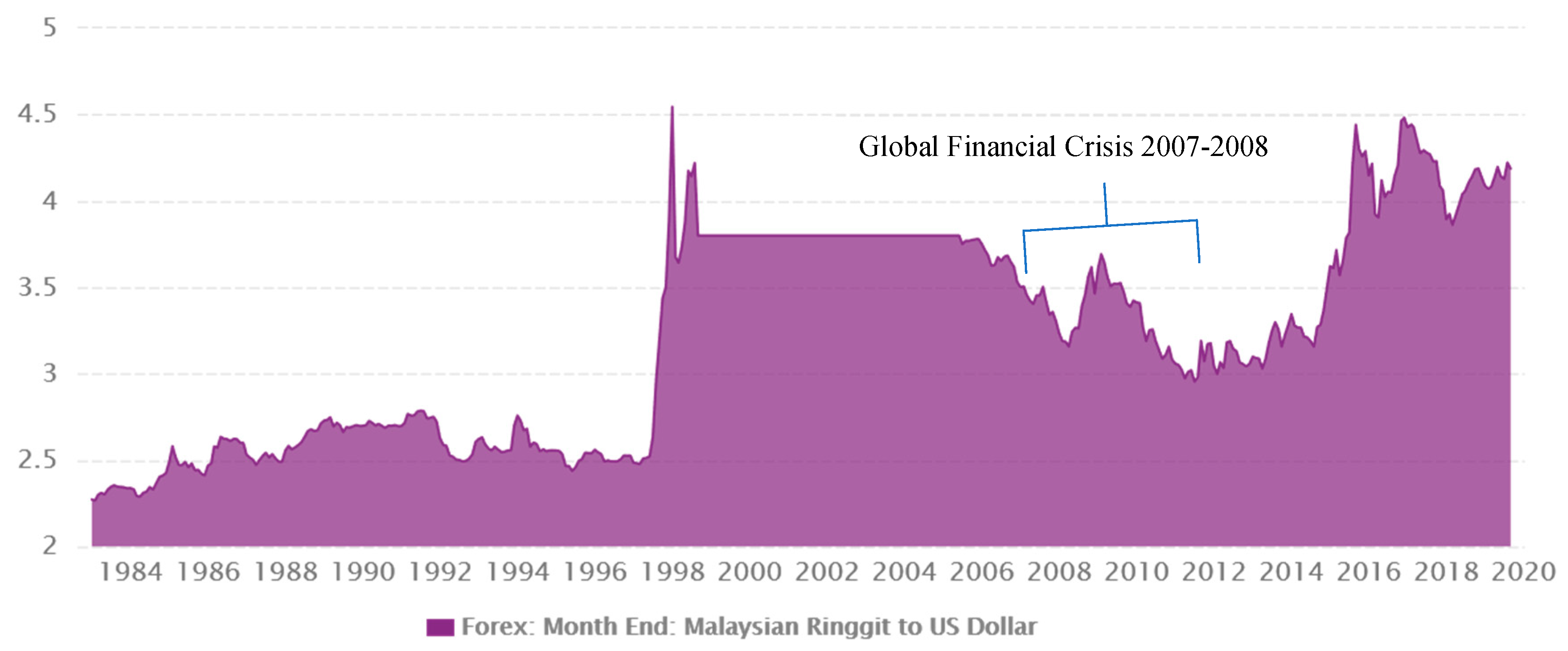
Malaysia, as an emerging economy, has maintained a starring record of macroeconomic management, for instance, [6]. The country needs a fiscal policy framework, which should be carefully designed to confirm that expenditures are consistent with social objectives and available for financing [7]. In 1981–1986 crises, Malaysia has experienced a severe current account deficit. The budget deficit as a percentage of Gross National Product (GNP) was historically high, up to 18% in 1983. The public debt at Gross Domestic Product (GDP) percentage sharply increased from 44% in 1980 to 103.4% in 1987. In the late 1990s, Malaysia faced heavy selling pressure on ringgits because of the Thai Baht depreciation in May 1997. In January 1998, Ringgit depreciated against the dollar by almost 50%. However, the low foreign debt experience of financial institutions made Malaysia policymakers unable to manage the situation. In short, fiscal profligacy was the main reason of macroeconomic imbalance in the first two crises, that is, 1981–1986 and 1997–1998. The first two crisis happened in Malaysia somewhat based on fiscal grounds, and financing sources of fiscal deficits. Malaysia, affected by the Asian crisis 1997 and the Global crisis 2007–2008 (see,

Table 1. Impact of global financial crises on Malaysia’s economy.

	2000	2001	2002	2003	2004	2005	2006	2007	2008	2009	2010
Growth of GDP %	8.9	0.5	5.4	5.8	6.8	5.3	5.8	6.5	4.7	−1.7	5.0
Consumers Price Index (CPI) %	1.5	1.4	1.8	1.2	1.4	3.1	3.6	2.0	5.4	0.6	2.0
Fiscal Deficit (at GDP %)	−6.6	−5.5	−5.8	−5.3	−4.1	−3.6	−3.3	−3.2	−4.8	−7.4	−5.6
Total public Debt (TPD) at GDP %	36.6	41.3	45.6	44.9	45.7	43.8	42.2	41.6	41.5	48.5	47.8
Foreign Debt (at TPD %)	15	16.7	22	19.7	16	13.1	10.3	7.3	6.6	4.3	4.5
Money Supply (M2)/GDP	100	103.4	100.9	102.5	113.4	118.9	126.7	124.1	121.9	145.6	148.6

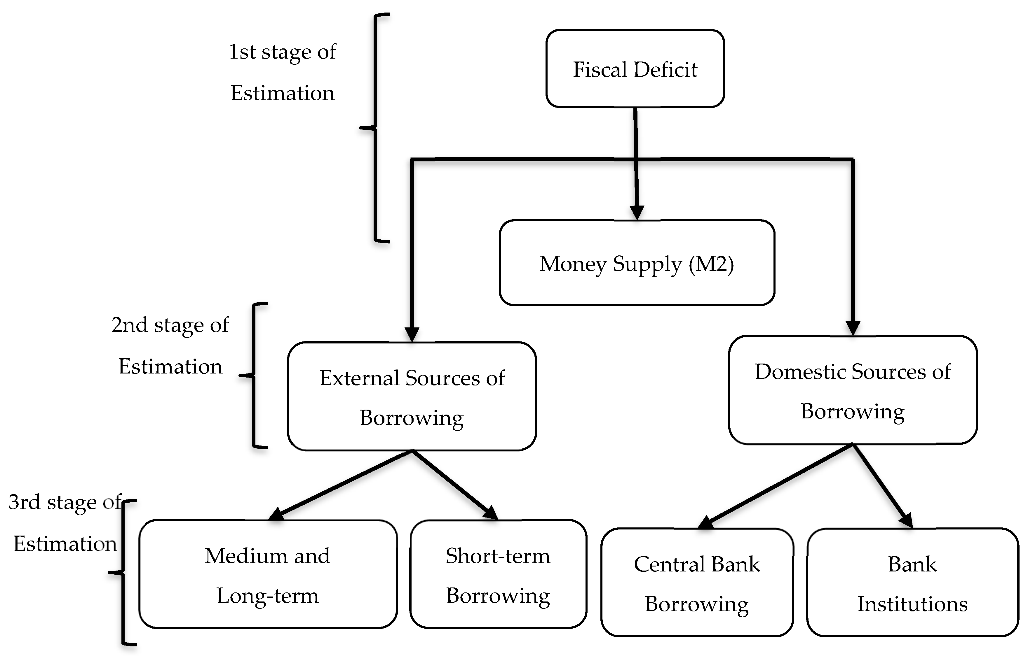
, and Figure 1), is planning to enrich the effectiveness of government expenditures through the application of zero-based budgeting, in which all expenditures will be justified for each new period, as reported in the annual report 2018 by Bank Negara [8]. The overall balance of the Federal Government budget is 3.7 percent of GDP, as per the report of the Ministry of Finance [9]. Fiscal deficit can be financed through many sources, for instance, printing of new money, domestic borrowing, and external borrowing. In Malaysia, domestic borrowing includes the Bank institution borrowing (commercial banks) and central bank borrowing, and these sources and more are highlighted by Bank Negara Annual reports. While in external borrowing, the most important are medium- and long-term borrowing and short-term borrowing. In past trends, Malaysia has faced a rising inflation of 5.44% and faced a fiscal deficit of 35,594 RM million (RM denotes the Malaysian currency symbol) in 2008 Q1 as per World Bank Data [10]. As mentioned earlier, there are sources of financing the fiscal deficit, but debt levels always exert extra pressures on the fiscal sustainability of public finances [11].

Consequently, to lessen this pressure and assuming fiscal sustainability as a constraint, it is essential to choose those sources which are less inflationary. There are several factors from supply side and demand side which can be responsible for inflation, like oil prices and food prices in the market. Now, the question is whether the fiscal deficit is inflationary in Malaysia? If it is inflationary, then which sources of financing the fiscal deficit are less inflationary? Ideally, at the time of fiscal deficit in the economy, the government covers the deficit with less inflationary sources. Sources with high inflation costs can make the economy in trouble. While discussing fiscal deficit and sources of financing and inflation, it is considered important to also discuss political instability in this study. As mentioned, political instability has been given less importance in studies, even though it causes many economic problems, and one of the critical economic problems is the inflation rate [12]. Political instability (PS) refers to fluctuations or variabilities in the political system which severely damage the economic system of a country. In Malaysia, political stability has specific challenges, such as institutional reforms, job-led growth, religious and racial issues, and national security challenges. In this study, political instability (PS) is considered as a moderator between fiscal deficit and inflation. The index range of PS is −2.5 (refers Not stable) to 2.5 (more Stable).

In general, several studies argued about fiscal deficit and inflation [3,13,14]. These arguments are based on theory, that is, Fiscal deficit causes an increase in money supply, inflation, which increases the interest rate and finally, crowds out the investment in the private sector. According to the Keynesian school of thought, budget deficit affects the interest rate, inflation through financing methods. Besides, the Monetarist school of thought argued that budget deficit affects money supply and inflation through financing methods. A plethora of studies has been done on the relationships of fiscal deficit and inflation [15,16,17,18,19].However, these studies have only analyzed the fiscal deficit and inflation as theoretically described in the fiscal theory of price, but another side of the fence has been ignored, which is the sources to finance the fiscal deficit and its inflation cost. It is essential to address the budget balance because, in the short run, it becomes crucial for the government to control inflation in the country [20]. Also, political instability has a significant relationship with rising inflation, as reported by Barugahara [21], Aisen & Veiga [22], and Telatar et al. [23]. As discussed earlier, the political instability means certain challenges in Malaysia, which is given less importance in the previous studies, even though it causes a high inflation rate [20,21]. So, it is quite important to know the impacts of fiscal deficit on inflation having political instability as a moderator. Further, from a technical perspective, the Autoregressive Distributed Lag (ARDL) technique has been used in previous studies to find out the long-run relationships, but its sensitivities are missing, for example [16,24]. Thus, this study re-estimates the model by incorporating Fully Modified Ordinary Least Squares (FMOLS), Dynamic Ordinary Least Squares (DOLS), and Canonical Cointegration Regression (CCR) techniques to find out the robustness of the estimates.

This study aims to investigate the relationship between fiscal deficit and inflation in Malaysia’s economy, along with long-run and short-run relationships. The second objective is to evaluate the sources, including external and internal, to finance the deficit with less impact on inflation. Also, the third objective of this study is to examine the political instability as a moderating variable between inflation and fiscal deficit in Malaysia.

This paper is structured as follows. Section 2 describes the findings of previous related studies, Section 3 explains the data sources and methodology, Section 4 presents the empirical findings, Section 5 discusses the empirical findings, and finally, Section 6 gives the concluding remarks.

2. Literature Review

Numerous studies have investigated the relationship between fiscal deficit and inflation with both time-series and panel data. Nguyen [15] examined the impacts of fiscal deficit and money supply (M2) on inflation in nine Asian countries and concluded that M2 and fiscal deficit have a positive and significant impact on inflation. Lin and Chu [16] applied dynamic quantile regression model under autoregressive distributive lag (ARDL) and investigated the fiscal deficit and inflation relationship in 91 countries from 1960–2006, empirical results showed that fiscal deficit could be inflationary when there is already inflation in the economy (high-inflation time) and can be less inflationary in low-inflation time. Sergey Pekarski [17] examined shifts in moderate and hyperinflation occurring because of shifts in monetary and fiscal policy by considering Laffer curve—represents the relationship between the tax rate and the amount of tax collected by governments, which is used to illustrate the Laffer’s argument that sometimes cutting tax rate can increase total revenue [25], and Olivera-Tanzi effect—an economic situation involving a period of high inflation and a decline in tax revenues, which can divide the budget deficit effect into two parts, one part, which is subject to negative inflation, and the second part, which is inflation proof. Graeve and Heideken [18] discussed anticipated inflation, which is strictly related to fiscal policy, and pointed out that warnings for fiscal inflation are always ignored in policies. The results suggested that fiscal inflation had already induced a 1.6 percent points increase in long-term inflation in 2001. Nandi [26] investigated the monetary policy and fiscal policy consistency and found that under high interest rate, passive monetary policy is consistent with fiscal policy. The study findings suggested the impact of fiscal policy on monetary policy; for instance, favorable fiscal policy can make monetary policy expansionary. The study highlighted the issue that there is a need for coordination between both policies. Ahmad and Aworinde [19] analyzed the relationship between fiscal deficit and inflation in twelve African countries using quarterly data by using asymmetric cointegration analysis, which is suitable for African countries with under-developed and imperfect financial markets system. The study exposed that fiscal deficit is inflationary in Africa, and there is a long-run relationship between fiscal deficits and inflation, indicating the importance of fiscal consolidation. Montes and Limba [27] analyzed fiscal transparency and its effects on inflation, inflation expectations, inflation volatility, and inflation expectations volatility in 82 developed and developing countries. Their findings suggested that countries could have low inflation volatility and low inflation expectations volatility as well as lower inflation and lower inflation expectations with a high level of fiscal transparency; especially in developing countries, fiscal transparency has a substantial impact on inflation. Hove et al. [28] studied the importance of institutional quality regarding the inflation target regime in emerging market economies. The study found that monetary policy is more effective in countries having good institutions. Canh [29] examined the effects of fiscal policy on economic growth under the contributions of internal and external debt levels in emerging market economies. The findings showed the fact that improvements in institutions can promote a huge crowd in the effects of fiscal policy and reported nonlinear effects of external debt on economic growth. Jalil et al. [30] tested the fiscal theory of price level in Pakistan covering the period from 1972 to 2012. The study exposed the fact that fiscal deficit is a significant contributor to inflation, along with other factors like interest rate, government sector borrowing, and private borrowing. Asterio [31] examined large fiscal deficits and public debt (by considering fiscal and budgetary shocks) and developed a macroeconometric model for the Greek economy. They have reported that the Greek government should try to reform fiscal programs which can boost the Greek economy. A similar study [32] investigated the impact of economic growth and external debt on fiscal deficit in Jordan, after using unit root and ARDL bound test, the empirical results showed that external debt has a negative impact on the budget deficit in Jordan. A related study reported the effects of a fiscal deficit on inflation in selected African Countries [33]. It concluded that in Nigeria, inflation is affected positively by the fiscal deficit in the short run and long run, while in South Africa and Kenya; there is a short run and adverse effects.

The review of studies shows that many studies have analyzed the relationship between fiscal deficit and inflation. However, the literature is lacking in the subject domain and shows a clear gap to fulfill. This study is considering domestic sources and external sources to finance the fiscal budget. The domestic sources include central bank and bank institutes, while the external sources include medium- and long-term loans and short-term loans. This study analyzes each of these sources of financing for fiscal budget and their corresponding inflation cost so that the policymakers can target the specific less inflationary sources to covers up the fiscal deficit.

3. Methodology

3.1. Data Source and Functional Form of the Models

The main source of Data for this study is the Bank Negara Malaysia covering the period from 2000 Q1 to 2018 Q4 with a sample size of 76, and the unit is RM million. Local currency has been used in recent studies in other economies, such as in Hussain and Haque [34]. This study is taking a quantitative research paradigm and using quarterly data to identify the changes in the trends (Figure 2). Variables are in log form (growth rate) and represented in small letters, except Consumers Price Index (CPI), as it is already in percentages.

CPI is the most commonly used indicator to gauge the level of prices. Here, CPI is used as a measure of inflation. Inflation (CPI) is defined as a function of fiscal deficit (FD) [2,24] and can be written as:

$$CPI=f\left(FD\right)$$

(1)

The above function states that fiscal deficit can be inflationary in nature. This study presents the modified version of this function by extending it to include the ways and means of financing the fiscal deficit in Malaysia. The government can finance the deficit by making changes in the money supply (M2), borrowing from domestic sources (DB) and external sources (ES). In addition, political instability (PS) is included as a moderator between inflation and the sources of financing, so the next equation can be denoted as:

$$CPI=f\left(PS,M2,DB,ES,GDP\right)$$

(2)

Domestic sources (DB) can be categorized into two forms: (1) Central bank borrowing (CBB), (2) Bank institutions borrowing (BIB), and the external sources can also be categorized into two forms: (1) Medium-and long-term borrowing (MLT), (2) Short-term borrowing (STL). Thus, the previous equation can be written as:

$$CPI=f(PS,M2,CBB,BIB,MLT,STL,GDP)$$

(3)

Variables Definitions

• Gross Domestic Product (GDP): GDP at current prices is the sum of gross value added by all resident producers in the economy plus any product taxes and minus any subsidies not included in the value of the products. It is calculated without making deductions for depreciation of fabricated assets or depletion and degradation of natural resources. The data are available in the local currency.
• Inflation: Consumer Price index (CPI) is used as an indicator of inflation. In the empirical analysis, CPI is the most frequently used variable for the price level in the economy [35].
• Fiscal deficit: Fiscal deficit is the difference between total revenue and expenditure during the fiscal year.
• Money supply (M2): M2 is defined as the sum of currency in circulation, other deposits with the central bank of Malaysia (Bank Negara), including resident foreign currency deposits with scheduled banks.
• Political instability (PS): Political instability estimates perceptions of the likelihood of political stability or politically motivated violence. This estimate gives the country’s score on the aggregate indicator, in units of standard normal distribution (i.e., ranging from −2.5 to 2.5).
• Central bank borrowing for budgetary support (CBB): It is the government source of borrowing from central bank of Malaysia (BNM) directly for fiscal deficit financing through printing of new money in economy or borrowing through ways and means advances.
• Bank institution borrowing (BIB): Bank borrowing for budgetary support is the borrowing of a government from banking sector within the economy during the fiscal year.
• Domestic borrowing (DB): Domestic borrowing includes the central bank and other bank institutions. In the study, domestic borrowing is categorized in two parts, central bank borrowing and bank institutions borrowing.
• External borrowing (EB): External borrowing for fiscal deficit financing includes two main categories: medium and long-term borrowing (MLT) and short-term borrowing (STL).

3.2. First Model

In the first model, inflation is used as a function of fiscal deficit [2]. The Gross Domestic Product (GDP) is considered as a control variable, and the money supply (M2) is used as an endogenous variable. The relationship between inflation and fiscal deficit is symbolically denoted as follows:

$$CP{I}_t={\alpha }_0+{\beta }_{1}F{D}_t+{\beta }_{2}GD{P}_t+{\beta }_{3}M{2}_t+{\epsilon }_t$$

(4)

The model domestic and external sources of financing are not included in the first model. This model is reflecting the direct effect of fiscal deficit on inflation.

3.3. Second Model

In the second model, the previous model is modified by substituting the FD with its sources of financing, that is, domestic borrowing (DB) and external borrowing (EB). Both sources are assumed as endogenous for comparison purposes. In addition, political instability (PS) is acting as a moderator between inflation and the external sources. Previously, studies reported that fiscal deficit leads to inflation if political instability (PS) is moderating this relationship, especially in developing and emerging economies [36,37]. Further, in most of the developing countries, the dominance of political instability ultimately contributes to large fiscal deficit [38]. In this study, political instability (PS) is incorporated as a moderator between inflation and sources of financing to check specifically the significance of the PS as a moderator. The second model can be written as:

$$CP{I}_t={\alpha }_0+{\beta }_{1}D{B}_t+{\beta }_{2}E{B}_t+{\beta }_{3}P{S}_t+{\beta }_{4}M{2}_t+{\beta }_{5}GD{P}_t+{\epsilon }_t$$

(5)

3.4. Third Model

In the third model, the subcategories of domestic sources, central bank borrowing (CBB), and Bank institutions borrowing (BIB), and subcategories of external sources, medium- and long-term borrowing (MLT) and short-term borrowing (STL), are included as a replacement for DB and EB. The third model is defined as follows:

$$CP{I}_t={\alpha }_0+{\beta }_{1}CB{B}_t+{\beta }_{2}BI{B}_t+{\beta }_{4}M{2}_t+{\beta }_{5}GD{P}_t+{\beta }_{6}P{S}_t+{\beta }_{7}ML{T}_t+{\beta }_{8}ST{L}_t+{\epsilon }_t$$

(6)

3.5. Econometric Techniques

3.5.1. Unit Root Test

This study used time-series data. Usually, time-series data illustrate trending behavior or the problem of nonstationarity. Consequently, it is necessary to remove such a stochastic behavior to get valid results. So, it is important or a pre-condition to test time-series properties to identify the stationarity at levels or at first difference and second difference. These analysis steps help to select a suitable model for data analysis. This study performs Augmented Dickey Fuller (ADF)—a well-known test for estimation of the integration order of variables [39].

3.5.2. Auto-Regressive Distributive Lag (ARDL) Model Bound Test for Cointegration

This study used the ARDL model to test the relationship between inflation and fiscal deficit [40]. The ARDL model provides two bounds of critical values, one for I(0) and the second for I(1), where I(0) refers to integrated at level zero, and the I(1) refers to integrated at level one. Therefore, the ARDL model avoids the deficiencies arising due to the classification of variables according to their integration order whether I(0) or I(1). In simple words, the ARDL model is possible to apply whether the variable in purely I(0) or I(1) or a mixture of both. The ARDL model has advantages against the traditional cointegration tests, such as the ARDL model is applicable even with the endogeneity issue of independent variables [41]. In addition, the ARDL models can be helpful to explore short-run dynamics and long-run relationships [42]. The unrestricted error correction representation of ARDL general model is presented as follows:

$$\mathsf{\Delta }{y}_t={\alpha }_0+{\beta }_0{y}_{t-1}+{\beta }_1{x}_{t-1}+{\displaystyle \sum }_{i=0}^p{\delta }_{1i}\mathsf{\Delta }{x}_{t-i}+{\displaystyle \sum }_{i=0}^p{\delta }_{2i}\mathsf{\Delta }{y}_{t-i}+{\epsilon }_t$$

(7)

where $\mathsf{\Delta }$ is the difference operator, p is the lag length, ${\epsilon }_t$ is the random error term. $Y_t$ represents the dependent variable, $x_t$ represents the independent variables. All variables can be tested for the null hypothesis of “No cointegration” by imposing restrictions on the joint significance. The null hypothesis can be tested through computing F-statistics and comparing it against the lower and upper bounds critical values [40]. If F-statistics is greater than the upper bound critical value at 5% level, then $H_0$ is rejected, it implies that there is a long-run relationship between the selected variables.

3.5.3. Fully Modified Ordinary Least Square (FMOLS)

Before concluding the findings, it is necessary to test the sensitivity of long-run parameters obtained from ARDL. This analysis re-estimates the model by applying FMOLS to find out the robustness of estimates [43]. FMOLS adopts the semiparametric approach in estimating the long-run parameters [44]. This technique provides consistent parameters even in the small sample size and overcomes the problem of endogeneity, serial correlation, and omitted variable bias. FMOLS adopts the semiparametric approach in estimating the long-run parameters and estimates a single cointegrating relationship, which is having a combination of I(1) variables [45].

3.5.4. Dynamic Ordinary Least Square (DOLS)

DOLS adopts a parametric approach in the estimation of a long-run relationship [46]. DOLS results are unbiased and efficient, controlling the endogeneity problem and adjusting the autocorrelation and residual non-normality. Mathematically it can be expressed as:

$$y_t=\alpha +c{x}_t+{\displaystyle \sum }_{i=-k}^{i=k}\varnothing \mathsf{\Delta }{X}_{t+i}+{ϵ}_t$$

(8)

where c represents the long-run elasticity, the term $\varnothing$ is the coefficient of leads and lags differences of I(1) regressors. These coefficients are called Nuisance parameters, they adjust to avoid endogeneity, autocorrelation, and non-normal residuals [47,48].

3.5.5. The Canonical Cointegration Regression (CCR)

Park [49] introduced canonical cointegration regression (CCR). This method can be used for testing cointegrating vectors in a model with an integrated process of I(1). This model is quite like FMOLS, though the difference is that CCR focusses on data transformation, while FMOLS is focusing on the transformation and parameters as well [50]. CCR is a single-equation regression that can be applied to multivariate regression without losing efficiency.

4. Empirical Results

4.1. Augmented Dickey Fuller Test

Variables from the first, second and third models have been tested for unit root by using Augmented Dickey Fuller test. The results show that first- and second-stage variables are stationary at I(1). Unit root results are mentioned with an intercept at levels while making it stationary at 1st difference. With intercept and trend it moves the value on the left side of normal distribution. Intercept with time trend is given below.

$$Y_t=\alpha +\delta t+\varnothing Y_{t-1}+{\epsilon }_t$$

(9)

The above equation includes a constant and deterministic time trend to capture the deterministic trend under the alternative. The inclusion of intercept and trend in the test regression shifts the distribution of $t_{\varnothing =1}$ and $T\left({\varnothing }^{\ast }-1\right)$ to the left [51]. For a sample size 76, the 5% left-tail critical values for $t_{\varnothing =1}$ and $T\left({\varnothing }^{\ast }-1\right)$ are now 1.34 and −3.31 (for variable M2). In FD, t-statistic value with a constant is negative while adding trend at first difference, the test regression further shifts the distribution to the left. Similar, trend is observed for variables DB, BIB, and STL. In the third stage, one variable, which is political instability (PS), is stationary at a level I(0) (see in

Table 2. Results of augmented Dickey Fuller (ADF) test.

	Variables	At Level	At First Difference	Conclusion
Dependent Variable	CPI	−0.089 (0.6376)	−6.4413 (0.0000) ***	I(1)
Stage 1 (Model in Equation (4))	M2	1.3441 (0.9977)	−3.3192 (0.0302) **	I(1)
	GDP	2.1967 (0.9997)	−4.9957 (0.0011) ***	I(1)
	FD	−1.6344 (0.4444)	−2.6253 (0.0121) **	I(1)
Stage 2 (Model in Equation (5))	DB	−0.5024 (0.8694)	−5.3468 (0.0006) ***	I(1)
	EB	0.136477 (0.9595)	−3.9580 (0.0087) ***	I(1)
Stage 3 (Model in Equation (6))	CBB	0.3183 (0.9719)	−7.0602 (0.0000) ***	I(1)
	BIB	−0.7007 (0.8224)	−5.3723 (0.0005) ***	I(1)
	MLT	0.2715 (0.9695)	−3.3799 (0.0269) **	I(1)
	STL	−0.1669 (0.9269)	−4.3220 (0.0042) ***	I(1)
	PS	−3.5060 (0.0203)	-	I(0)

Note: all variables are integrated at level 1. Value in parenthesis shows p-values. ***, ** representing stationary at level 1% and level 5%, respectively. Rest values are t-statistic values. DB, EB, CBB, BIB, MLT, STL, PS (All variables defined in Section 3.1.).

).

4.2. First Stage Estimation

The first model (Equation (4)) has inflation as a dependent variable and fiscal deficit, GDP, and M (money supply) as independent variables. ARDL bound test for cointegration has been performed to analyze the long-run relationship between inflation and fiscal deficit. The model selection method is based on the Akaike information criterion (AIC). The results are listed in

Table 3. Results of bound test of cointegration.

Test Statistics	Value	K
F-statistics	5.40	3
Critical Value Bounds
Significance	I0	I1
10%	2.37	3.2
5%	2.79	3.67
1%	3.65	4.66

. ARDL included automatic lag selection (four lags). The null of no cointegration may not be accepted at 1% level of significance, as F-statistics (5.40) lie outside the upper bound 4.66. Therefore, the long-run relationship is satisfied.

4.2.1. The Error Correction Mechanism (ECM) of ARDL

The ECM of the ARDL model shows short-run fluctuations along with error correction. The results of ECM are given in

Table 4. Results of error-correction mechanism.

Variable	Coefficient	Std. Error	t-Statistics	Prob.
$\mathsf{\Delta }$fd	5.58	2.96	1.88	0.06 *
$\mathsf{\Delta }$m2	−11.22	7.70	−1.45	0.15
$\mathsf{\Delta }$gdp	43.43	7.93	5.47	0.00 ***
ECT (−1)	−0.22	0.04	−5.29	0.00 ***
R2	0.56	S.E of regression	0.06

Note: ***, **, * representing level of significance at 1%, 5%, and 10% respectively. ‘Prob.’ denotes probability, and it refers to the p-values. S.E (refers standard error), ECT (error correction term).

. According to the short-run analysis, fiscal deficit plays a significant role in determining inflation as it is statistically significant at 6%. The money supply is insignificant and negatively related to the inflation rate in short run. Money supply control is not required to reduce inflation in the short run. Previous studies have reported negative relationships between money supply and inflation [52,53,54]. GDP is highly contributing to inflation by 43.43 units if there is 1 unit increase in GDP. Correction in the error is 22 percent in every quarter of the year. However, based on the analysis, we can say that the fiscal deficit is inflationary. In the next step, after testing the long-run relationship and short-run error correction between variables through a bound test and ECM, respectively, it is important to know the elasticities of long-run variables by cointegration regression.

4.2.2. Cointegration Regression Analysis

Cointegration regression analyses re-estimate the model by employing FMOLS, CCR, and DOLS to find the robustness of the estimates. This study has considered the robustness of long-run parameters by estimating the coefficients through FMOLS, DOLS, and CCR. The long-run elasticities are almost as same as the ARDL in signs and significance (see in

Table 5. Results of cointegration regression analysis (long-run coefficients).

Variable	ARDL	FMOLS	DOLS	CCR
C	4.07 (3.56)	10.53 (10.20)	6.88 (8.91)	10.03 (10.07)
Gdp	−26.32 * (15.90)	−1.53 (1.44)	−1.004 (1.24)	−1.44 (1.41)
Fd	5.75 ** (2.90)	1.09 *** (0.33)	1.01 *** (0.28)	1.04 *** (0.31)
m2	25.04 * (13.46)	2.14 * (1.26)	1.66 (1.09)	2.03 * (1.21)
Long-run variance		0.04	0.01	0.04
R2	0.85	0.21	0.76	0.21

Note: ***, **, * representing level of significance at 1%, 5%, and 10%, respectively. The values in the parentheses are standard errors. Autoregressive Distributed Lag (ARDL), Fully Modified Ordinary Least Squares (FMOLS), Dynamic Ordinary Least Squares (DOLS), and Canonical Cointegration Regression (CCR).

). The fiscal deficit is significant in ARDL, FMOLS, DOLS, and CCR. But it can be observed that the R² value from FMOLS and CCR is quite a lot less, while DOLS and ARDL R² values are good. It can be because of the semiparametric approach of FMOLS. The FMOLS and CCR almost give the same results with the long-run variance 0.04. DOLS model is a good fit for the model in Equation (4), having low long-run variance value. The ARDL fd, GDP and m are statistically significant. GDP and inflation are having an inverse relationship, as mentioned in [55]. Inflation reduces the level of investment, which adversely affects the economic growth of a country [56,57,58]. The money supply is positively related to inflation.

4.3. Second Stage of Estimation

In the second stage of estimation, fiscal deficit is replaced by external and domestic sources of financing. Most importantly, political stability has been used as a moderator between inflation and its source of financing. It can be observed specifically which source of financing is contributing more to the inflation and political instability (PS) effect on inflation. In the second model (Equation (5)), four variables are used as dependent variables, that is, external sources of financing and domestic sources of financing, money supply, and Gross domestic product.

The results of the ADRL bound test are shown in

Table 6. Results of bound test of cointegration.

Test Statistics		Value	K
F-statistics		10.38	4
	Critical value Bounds
Significance		I0	I1
10%		2.2	3.09
5%		2.56	3.49
1%		3.29	4.37

. The null of no cointegration may not be accepted at a 1% level of significance, as F-statistics (10.38) lies outside the upper bound 4.37. Therefore, the long-run relationship is confirmed.

4.3.1. The Error-Correction Mechanism (ECM) of ARDL

The domestic borrowing is highly insignificant, as the corresponding obtained coefficient value is 0.03, as shown in

Table 7. Results of error-correction mechanism of ADRL.

Variable	Coefficient	Std.Error	t-Statistics	Prob.
$\mathsf{\Delta }eb$	1.31	0.31	4.13	0.00 ***
$\mathsf{\Delta }db$	0.03	0.35	0.10	0.91
$\mathsf{\Delta }$gdp	15.85	1.67	9.46	0.00 ***
$\mathsf{\Delta }PS$	−0.44	0.22	−2.002	0.04 **
ECT(-1)	−0.11	0.01	−8.20	0.00 ***
R2	0.61	S.E of regression	0.06

Note: ***, **, * representing level of significance at 1%, 5%, and 10%, respectively. “Prob.” denotes probability, and it refers to the p-values.

. The external source of borrowing is significant and impactful as its coefficient value is 1.31. Political instability is statistically significant and negatively related to inflation in the short run. ECT term representing the short-run adjustments in equilibrium as 11% convergence is possible to the equilibrium quarterly.

4.3.2. Cointegration Regression Analysis

The ARDL, FMOLS, DOLS, and CCR show the significance of domestic borrowing and have a negative relationship with inflation, as shown in the long-run analysis in

Table 8. Results of Cointegration Regression Analysis (Long-run Coefficients).

Variable	ARDL	FMOLS	DOLS	CCR
c	−61.68 * (31.90)	−21.18 *** (5.82)	−10.03 (15.19)	−7.45 (15.06)
gdp	7.96 * (4.57)	2.43 *** (0.66)	0.55 (2.13)	0.40 (2.17)
PS	−0.47 (0.71)	0.27 (0.34)	0.57 (0.38)	0.30 (0.28)
m2	−1.79 (4.57)	1.88 (1.90)	2.46 (1.77)	2.03 * (1.21)
eb	−0.69 (0.58)	−0.39 (0.29)	−0.52 (0.33)	−0.3 (0.27)
db	−3.73 *** (1.39)	−1.32 ** (0.55)	−1.76 *** (0.51)	−1.31 ** (0.53)
Long-run variance		0.04	0.01	0.04
R2	0.90	0.30	0.75	0.30

Note: ***, **, * representing level of significance at 1%, 5%, and 10%, respectively. The values in the parentheses are standard errors. Variables defined in Section 3.1.

. External borrowing is insignificant in all techniques and has a negative relationship with inflation. The external borrowing may be positive if utilized for productive purposes (investment), it can put negative effects on the economy if utilized for private or public consumption [59]. So external borrowing can be more inflationary if utilization is not productive. In the long-run analysis, political instability is not statistically significant. The DOLS and ARDL R² values are 75% and 90%, respectively.

4.4. Third Stage of Estimation

In the third stage of estimation, domestic borrowing and external borrowing are further divided into two categories to get the specific results. The domestic borrowing includes bank institution borrowing and central bank borrowing; while the external borrowing includes medium- and long-term borrowing and short-run borrowing. The results for ARDL bound test for long-run relationships are given in

Table 9. Results of bound test of cointegration.

Test Statistics	Value	K
F-Statistics	5.18	7
Critical value Bounds
Significance	I0	I1
10%	1.92	2.89
5%	2.17	3.21
1%	2.73	3.9

. The null of no cointegration is rejected at a 1% level of significance, as F-statistics (5.18) lies outside the upper bound 3.9. Therefore, the long-run relationship is satisfied.

4.4.1. The Error Correction Mechanism (ECM) of ARDL

The variables bib and cbb are significant but have less impact on inflation as 0.004 and 0.003, respectively, as shown in the short-run results in

Table 10. Results of error-correction mechanism.

Variable	Coefficient	Std.Error	t-Statistics	Prob.
$\mathsf{\Delta }bib$	0.004	0.002	2.03	0.04 **
$\mathsf{\Delta }cbb$	0.003	0.001	3	0.00 ***
$\mathsf{\Delta }gdp$	35.38	8.31	4.25	0.00 ***
$\mathsf{\Delta }PS$	0.85	1.01	0.84	0.40
$\mathsf{\Delta }m2$	10.74	7.86	1.36	0.17
$\mathsf{\Delta }$mlt	9.09	3.76	2.41	0.01 **
$\mathsf{\Delta }$stl	4.83	2.37	2.03	0.04 **
ECT(-1)	−0.17	0.02	−7.30	0.00 ***
R2	0.60	S.E of regression	0.31

Note: ***, **, * representing level of significance at 1%, 5%, and 10%, respectively.

. The relationships of cbb and bib with inflation are positive. From external sources, the variables mlt and stl are both significant and have a large impact on inflation. In addition, PS is highly insignificant in this model (refers to Equation (6)). ECT term shows a 17% error correction in the model per quarter.

4.4.2. Cointegration Regression Analysis

As mentioned earlier, this study considered to estimate long-run elasticities using FMOLS, DOLS, and CCR. The variable bib (bank institution borrowing) is significant in all methods, having less impact on inflation, and the variable mlt (medium- and long-term borrowing) has a significant and negative impact on inflation, see in

Table 11. Results of cointegration regression analysis (long-run coefficients).

Variable	ARDL	FMOLS	DOLS	CCR
c	760.44 (464.47)	−128.22 * (71.26)	136.40 (103.44)	−117.007 (71.98)
bib	0.001 ** (0.0007)	0.007 *** (0.002)	0.001 *** (0.0002)	0.007 *** (0.002)
Cbb	0.001 (0.0009)	0.0017 (0.0019)	0.004 (0.003)	0.002 (0.001)
PS	1.10 (3.20)	2.29 (1.42)	0.6 (1.72)	2.15 * (1.16)
m2	72.97 * (40.14)	−5.15 (8.79)	46.48 *** (15.89)	−3.38 (9.13)
gdp	−102.56 * (60.12)	14.77 (10.03)	-36.06 (16.50)	12.85 (10.44)
mlt	−3.57 (9.47)	−5.67 * (3.07)	13.05 * (6.50)	−5.32 * (3.03)
stl	9.18(9.31)	3.83 (2.63)	9.43 * (5.22)	3.68 (2.45)
Long-run variance		0.8	0.3	0.08
R2	0.89	0.47	0.83	0.45

Note: ***, **, * representing level of significance at 1%, 5%, and 10%, respectively. Values mentioned in parenthesis are standard errors.

. The variables bib and cbb are less-inflationary; while the subcategories of external sources, stl and mlt are inflationary. A negative relationship between external borrowing and inflation was reported in previous studies, like [60] and [59], showing that external debt and inflation could have negative effects. External borrowing causes a rise in government expenditures and in that case, the inflation rate may get increased. However, the negative sign is reflecting the weak moderate inflation, (i.e., moderate inflation used as a proxy of macroeconomic stability in [19]). Such situations occur when governments consume a large portion of external debt on unproductive activities, which is diminishing the moderate inflation or macroeconomic stability and putting inflationary pressures. Referring to the results reported in Table 8 and Table 11, the domestic borrowing (db), medium- and long-term borrowing (mlt) reflect that a significant portion of borrowing is consumed by the government on unproductive activities, producing a significant rise in inflation. In the long run, external sources are more sensitive to inflation. In this model (refers to Equation (6)), the DOLS (parametric) R² value is higher than the FMOLS and the CCR values; while the R² value obtained for ARDL is 89%.

5. Discussion

Numerous studies have reported the relationship between inflation and fiscal deficit and concluded different findings [16,19,29,30]. Theoretically, the fiscal deficit is inflationary, but the impact and significance of its source of financing on inflation are varied. The analysis of this study is carried out in three stages of estimation. In the first-stage estimation, the model in Equation (4) is used; in the second-stage estimation, the model in Equation (5) is used; and in the final third-stage estimation, the model in Equation (6) is tested. In the first model, which can be called in general a model, inflation is depending on the overall fiscal deficit, money supply, and the GDP. Through the ARDL bound test, it is confirmed that there is a long-run relationship between inflation and fiscal deficit. While analyzing the short-run estimation, there is also a short-run relationship between inflation and fiscal deficit, but it is significant at 6%. In this study, after finding the short-run and the long-run relationship, the sensitivity of parameters is also estimated by using ARDL, FMOLS, DOLS, and CCR techniques. The coefficient of fiscal deficit is 5.75 in ARDL, 1.09 in FMOLS, 1.01 in DOLS, and 1.04 in CCR findings. All coefficients are positive, as expected, and significant at 1% and 5%. Increasing fiscal deficit implies an increase in inflation. Malaysia’s economy is facing a fiscal deficit, and then obviously, the government must face its inflation cost as well. In the same model, the money supply has shown a significant impact on inflation. Due to the fiscal deficit, a country may print new money, which can create inflation. As Lin and Chu [16] discussed, if inflation is already high, then the fiscal deficit may produce more inflation, but on the other hand, the fiscal deficit can be less inflationary in a steady inflation period.

In the second stage of estimation, the fiscal deficit is replaced by two main sources of financing, that is, the external source of borrowing and domestic source of borrowing, along with political instability as a moderator. The political instability is not included in the first stage of estimation because in the first stage, the aim is to find out the overall impact of fiscal deficit on inflation, GDP, and Money supply. In the second stage, it can be explicitly observed how the political instability moderates the relationship between the sources of financing and inflation, see Table 7. Hence, according to the findings, there is a long-run relationship between the sources of financing and inflation. In the short-run analysis, the external sources of borrowing have also shown a short-run relationship with inflation, when the government borrows money from the external sources to cover up the fiscal deficit, affecting the money supply in the country’s economy and causing inflation in the short run. On the other hand, domestic borrowing has a long-run relationship, if the government takes domestic borrowing, which may not be in a large amount and may not be affecting in the short run, but in the long-run, it is significantly inflationary, see Table 8. Political instability is also one of the critical factors which can affect inflation. Recently, the Malaysian government has changed through their democratic process, resulting in changes in the revenue structure and the regulations, which affected the price level in the market.

In the third stage of estimation, the external sources, including short-, medium-, and long-term borrowing, are having a short-run relationship with inflation. The short-term borrowing can be helpful for the government to support the fiscal deficit because the short-term borrowing is less-inflationary relative to medium- and long-term borrowing. In the long-term analysis, it is very clear from the findings that the central bank borrowing and the Bank institution borrowing have a less and significant impact on inflation. Utilization of these funds must be productive when the government funds fail to achieve development policy over the long term, and it can seriously damage the fiscal stability [61]. On the other hand, the government is relying on medium- and long-term borrowing and short-term borrowing to achieve the gap in the fiscal deficit, which is inflationary. In specific analysis (after dividing the external and domestic sources), political instability is not significantly affecting the market price levels.

6. Conclusions

The primary aim of this study is to explore the less inflationary sources to finance the fiscal deficit and to analyze the long-run and short-run relationships between sources of financing fiscal deficit and inflation. Further, political instability is used as a moderator between sources of financing and inflation to check its significance. The findings from the first-stage analysis conclude that the fiscal deficit is inflationary in the country. From the second stage of estimation, this study concludes that political instability moderates the link between sources of financing and inflation. The external source of financing may be inflationary in the short run. Similarly, from the third stage of estimation, the study concludes that central bank borrowing and bank institution borrowing (domestic sources) have less impact on inflation, medium- and long-term borrowing are more sensitive relative to the short-run borrowing. In the short run, the government can rely on external sources for short-term borrowing (as they are less inflationary in the short run), and for a long-term policy, domestic sources for central bank borrowing and bank borrowing can be used, as these sources are found less inflationary.

The findings of this study recommend that Malaysia’s Government should rely on domestic borrowing for long-term bases and external borrowing (short-term loans) for short-term periods as they are found to be less inflationary. Besides, the study highly recommends the fiscal consolidation for the Malaysian’s economy.

References

1. Faraglia, E.; Marcet, A.; Oikonomou, R.; Scott, A. The impact of debt levels and debt maturity on inflation. Econ. J. 2013, 123, F164–F192. [Google Scholar] [CrossRef] [Green Version]
2. Catão, L.A.V.; Terrones, M.E. Fiscal deficits and inflation. J. Monet. Econ. 2005, 52, 529–554. [Google Scholar] [CrossRef] [Green Version]
3. Maio Bulawayo, F.C.; Seshamani, V. The Impact of Budget Deficits on Inflation in Zambia. J. Econ. 2018, 6, 13–23. [Google Scholar] [CrossRef]
4. Sargent, T.J.; Wallace, N. Rational expectations and the theory of economic policy. Ration. Expect. Econom. Pract. 1981, 1, 199–214. [Google Scholar]
5. Fisher, I. The Purchasing Power of Money: Its’ Determination and Relation to Credit Interest and Crises; Cosimo, Inc.: New York, NY, USA, 2006. [Google Scholar]
6. Bowie, A.; Unger, D.; Unger, D. The Politics of Open Economies: Indonesia, Malaysia, the Philippines, and Thailand; Cambridge University Press: Cambridge, UK, 1997; Volume 4. [Google Scholar]
7. Athukorala, P.-C. Malaysian Economy in THREE Crises; The Australian National University: Canberra, Australia, 2010. [Google Scholar]
8. Yunus, N.S. Annual Report of Bank Negara Malaysia; Bank Negara: Kuala Lumpur, Malaysia, 2018. [Google Scholar]
9. Farisan, W. Fiscal Updates; Ministry of Finance: Putrajaya, Malaysia, 2017.
10. World Bank Data. Available online: https://data.worldbank.org/country/malaysia (accessed on 3 September 2019).
11. Popescu, M.; Militaru, E.; Cristescu, A.; Vasilescu, M.; Maer Matei, M. Investigating health systems in the European Union: Outcomes and fiscal sustainability. Sustainability 2018, 10, 3186. [Google Scholar] [CrossRef] [Green Version]
12. Aisen, A.; Veiga, F.J. Political instability and inflation volatility. Public choice 2008, 135, 207–223. [Google Scholar] [CrossRef] [Green Version]
13. Devapriya, T.N.K.; Ichihashi, M. How Does the Budget Deficit Affect Inflation in Sri Lanka; IDEC Discussion Paper: Hiroshima, Japan, 2012. [Google Scholar]
14. Oseni, I.O.; Sanni, H.Y. Does Fiscal Deficit Granger Cause Impulsiveness in Inflation Rate in Nigeria? Acta Univ. Danubius. Œconomica 2016, 12, 208–216. [Google Scholar]
15. Nguyen, B. Effects of fiscal deficit and money M2 supply on inflation: Evidence from selected economies of Asia. J. Econ. Financ. Adm. Sci. 2015, 20, 49–53. [Google Scholar] [CrossRef] [Green Version]
16. Lin, H.-Y.; Chu, H.-P. Are fiscal deficits inflationary? J. Int. Money Financ. 2013, 32, 214–233. [Google Scholar] [CrossRef]
17. Pekarski, S. Budget deficits and inflation feedback. Struct. Chang. Econ. Dyn. 2011, 22, 1–11. [Google Scholar] [CrossRef] [Green Version]
18. De Graeve, F.; von Heideken, V.Q. Identifying fiscal inflation. Eur. Econ. Rev. 2015, 80, 83–93. [Google Scholar] [CrossRef] [Green Version]
19. Ahmad, A.H.; Aworinde, O.B. Are fiscal deficits inflationary in African countries? A new evidence from an asymmetric cointegration analysis. N. Am. J. Econ. Financ. 2019, 50. [Google Scholar] [CrossRef]
20. Tsen, W.H. External Balance and Budget in Malaysia. Asian Acad. Manag. J. Account. Financ. 2014, 10, 37–54. [Google Scholar]
21. Barugahara, F. The impact of political instability on inflation volatility in Africa. S. Afr. J. Econ. 2015, 83, 56–73. [Google Scholar] [CrossRef]
22. Aisen, A.; Veiga, F.J. Does political instability lead to higher inflation? A panel data analysis. J. Money Credit Bank. 2006, 38, 1379–1389. [Google Scholar] [CrossRef] [Green Version]
23. Telatar, E.; Telatar, F.; Cavusoglu, T.; Tosun, U. Political instability, political freedom and inflation. Appl. Econ. 2010, 42, 3839–3847. [Google Scholar] [CrossRef]
24. Ali, K.; Khalid, M. Sources to Finance Fiscal Deficit and Their Impact on Inflation: A Case Study of Pakistan. Pak. Dev. Rev. 2019, 58, 27–43. [Google Scholar] [CrossRef] [Green Version]
25. Laffer, A.B. The Laffer curve: Past, present, and future. Backgrounder 2004, 1765, 1–16. [Google Scholar]
26. Nandi, A. Fiscal Deficit Targeting alongside Flexible Inflation Targeting. J. Asian Econ. 2019, 62, 1–18. [Google Scholar] [CrossRef]
27. Montes, G.C.; da Cunha Lima, L.L. Effects of fiscal transparency on inflation and inflation expectations: Empirical evidence from developed and developing countries. Q. Rev. Econ. Financ. 2018, 70, 26–37. [Google Scholar] [CrossRef]
28. Hove, S.; Tchana, F.T.; Mama, A.T. Do monetary, fiscal and financial institutions really matter for inflation targeting in emerging market economies? Res. Int. Bus. Financ. 2017, 39, 128–149. [Google Scholar] [CrossRef] [Green Version]
29. Phuc Canh, N. The effectiveness of fiscal policy: Contributions from institutions and external debts. J. Asian Bus. Econ. Stud. 2018, 25, 50–66. [Google Scholar] [CrossRef] [Green Version]
30. Jalil, A.; Tariq, R.; Bibi, N. Fiscal deficit and inflation: New evidences from Pakistan using a bounds testing approach. Econ. Model. 2014, 37, 120–126. [Google Scholar] [CrossRef]
31. Asteriou, D.; Lalountas, D.A.; Siriopoulos, C. A Small Macro-econometric Model for Greece: Implications about the Sustainability of the Greek External Debt. SSRN 2011, 1884905. [Google Scholar] [CrossRef]
32. Al-Qudah, A.M.; Jaradat, M.A. Economic Growth, External Debt and Budget Deficit in Jordan: ARDL Approach. Sciences 2018, 7, 151–165. [Google Scholar]
33. Olubiyi, E.A.; Bolarinwa, M.A. Fiscal deficit and inflation rate in selected African Regional Blocs: A comparative analysis. Turk. Econ. Rev. 2018, 5, 89–101. [Google Scholar]
34. Hussain, M.; Haque, M. Fiscal deficit and its impact on economic growth: Evidence from Bangladesh. Economies 2017, 5, 37. [Google Scholar] [CrossRef] [Green Version]
35. Mankiw, N. Principles of Macroeconomics; Cengage Learning: New York, NY, USA, 2006. [Google Scholar]
36. Baldacci, E.; Gupta, S.; Mati, A. Political and fiscal risk determinants of sovereign spreads in emerging markets. Rev. Dev. Econ. 2011, 15, 251–263. [Google Scholar] [CrossRef]
37. Cox, G.W.; Weingast, B.R. Executive constraint, political stability, and economic growth. Comp. Political Stud. 2018, 51, 279–303. [Google Scholar] [CrossRef]
38. Feng, Y. Political freedom, political instability, and policy uncertainty: A study of political institutions and private investment in developing countries. Int. Stud. Q. 2001, 45, 271–294. [Google Scholar] [CrossRef]
39. Dickey, D.A.; Fuller, W.A. Distribution of the estimators for autoregressive time series with a unit root. J. Am. Stat. Assoc. 1979, 74, 427–431. [Google Scholar]
40. Pesaran, M.H.; Shin, Y.; Smith, R.J. Bounds testing approaches to the analysis of level relationships. J. Appl. Econom. 2001, 16, 289–326. [Google Scholar] [CrossRef]
41. Alam, I.; Quazi, R. Determinants of capital flight: An econometric case study of Bangladesh. Int. Rev. Appl. Econ. 2003, 17, 85–103. [Google Scholar] [CrossRef]
42. Pattichis, C.A. Price and income elasticities of disaggregated import demand: results from UECMs and an application. Appl. Econom. 1999, 31, 1061–1071. [Google Scholar] [CrossRef]
43. Phillips, P.C.; Hansen, B.E. Statistical inference in instrumental variables regression with I (1) processes. Rev. Econ. Stud. 1990, 57, 99–125. [Google Scholar] [CrossRef]
44. Priyankara, E. The Long-run Effect of Services Exports on Total Factor Productivity Growth in Sri Lanka: Based on ARDL, FMOLS, CCR, and DOLS Approaches. Int. J. Acad. Res. Bus. Soc. Sci. 2018, 8, 233–253. [Google Scholar] [CrossRef]
45. Manap, T.A.A. Stability of long-run money demand function: Evidence from Malaysia. J. Econ. Manag. 2009, 17, 261–285. [Google Scholar]
46. Stock, J.H.; Watson, M.W. A simple estimator of cointegrating vectors in higher order integrated systems. Econom. J. Econom. Soc. 1993, 61, 783–820. [Google Scholar] [CrossRef]
47. Herzer, D.; Nowak-Lehmann, D. Export diversification, externalities and growth: Evidence for Chile. In Proceedings of the German Development Economics Conference, Berlin, Germany, 12 December 2006; pp. 1–24. [Google Scholar]
48. Herzer, D.; Nowak-Lehnmann, D.F. What does export diversification do for growth? An econometric analysis. Appl. Econ. 2006, 38, 1825–1838. [Google Scholar] [CrossRef]
49. Park, J.Y. Canonical cointegrating regressions. Econom. J. Econom. Soc. 1992, 60, 119–143. [Google Scholar] [CrossRef]
50. Adom, P.K.; Amakye, K.; Barnor, C.; Quartey, G. The long-run impact of idiosyncratic and common shocks on industry output in G hana. OPEC Energy Review 2015, 39, 17–52. [Google Scholar] [CrossRef]
51. Levin, A.; Lin, C.-F.; James Chu, C.-S. Unit root tests in panel data: asymptotic and finite-sample properties. J. Econom. 2002, 108, 1–24. [Google Scholar] [CrossRef]
52. Cao, T. Paradox of Inflation: The Study on Correlation between Money Supply and Inflation in New Era; Arizona State University: Arizona, AZ, USA, 2015. [Google Scholar]
53. Tang, C.F.; Lean, H.H. Is the Phillips curve stable for Malaysia? New empirical evidence. Malays. J. Econ. Stud. 2007, 44, 95–105. [Google Scholar]
54. Cheng, M.-Y.; Tan, H.-B. Inflation in Malaysia. Int. J. Soc. Econ. 2002, 29, 411–425. [Google Scholar] [CrossRef]
55. Berument, H.; Inamlik, A.; Olgun, H. Inflation and growth: Positive or negative relationship? J. Appl. Sci. 2008, 8, 192–204. [Google Scholar] [CrossRef]
56. Mamo, F. Economic Growth and Inflation: A Panel Data Analysis; Södertörn University: Flemingsberg, Sweden, 2012. [Google Scholar]
57. Fischer, S. The role of macroeconomic factors in growth. J. Monet. Econ. 1993, 32, 485–512. [Google Scholar] [CrossRef] [Green Version]
58. Muritala, T. Investment, inflation and economic growth: empirical evidence from Nigeria. Res. J. Financ. Account. 2011, 2, 68–76. [Google Scholar]
59. Sulaiman, L.; Azeez, B. Effect of external debt on economic growth of Nigeria. J. Econ. Sustain. Dev. 2012, 3, 71–79. [Google Scholar]
60. Mweni, F.; Njuguna, A.; Oketch, T. The Effect of External Debt on Inflation Rate in Kenya, 1972-2012. Int. J. Financ. Res. 2016, 7. [Google Scholar] [CrossRef] [Green Version]
61. Bethlendi, A.; Lentner, C. Subnational Fiscal Consolidation: The Hungarian Path from Crisis to Fiscal Sustainability in Light of International Experiences. Sustainability 2018, 10, 2978. [Google Scholar] [CrossRef] [Green Version]
Figure 1. Trend in Malaysian currency against US Dollar (Source: Bank Negara Malaysia).
Sustainability 12 00366 g001
Figure 2. Fiscal deficit (FD) and sources of financing, that is, the printing of new money (Money Supply), external borrowing, and domestic borrowing.
Sustainability 12 00366 g002