Dynamic Models for Exploring the Resilience in Territorial Scenarios


Abstract
1. Introduction
2. State of Art of Resilience and Urban Resilience
3. Dynamic Models in the Decision-Making Process
3.1. Urban Simulation Models
3.2. System Dynamics Model
3.2.1. Methodological Background and State of Art
- Exponential growth or decline, which is characterized by only positive or only negative feedbacks;
- Goal-seeking behavior, which is created by first-order negative feedback;
- S-shaped growth. This behavior, over time, is created by a combination of positive and negative feedback loops. In this case, both loops struggle for dominance until the struggle ends with a long-term equilibrium;
- Oscillations. This is one of the most common types of dynamic behaviors in the world and it can have different forms, such as (1) sustained oscillations; (2) damped oscillations; (3) exploded oscillations; (4) chaos. The structure that creates oscillations is a combination of negative feedback loops and delay.
3.2.2. Illustrative Example
- (1)
- “HWS” is the annual household’s waste emission;
- (2)
- “DSWE” is the domestic solid waste emission.
3.3. Lotka–Volterra Cooperative Systems
3.3.1. Methodological Background and State of Art
- if a12, a21 > 0, benefits from the presence of the second state variable , then Lotka–Volterra models are defined as “cooperative”;
- if a12, a21 < 0, the first state variable competes with the second state variable, then Lotka–Volterra models are “competitive”;
- if a12 < 0 (prey), a21 > 0 (predator), it means that the two variables are opposite, then Lotka–Volterra models are “prey/predator”.
| a1 = b − c | b1 = −b | a12 = 0 | I1 = 0 |
| a2 = d − f | b1 = −d | a21 = f | I2 = 0 |
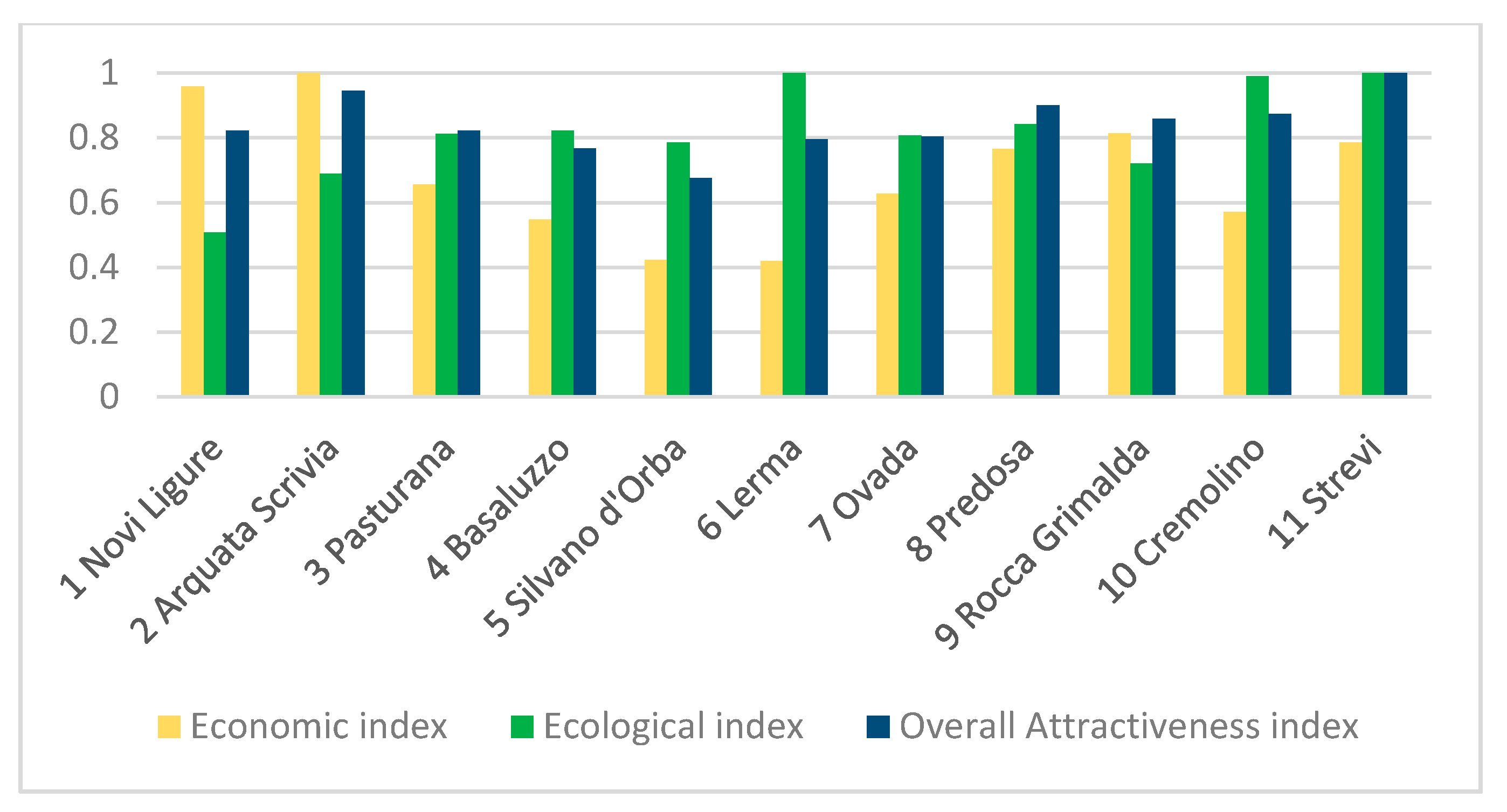
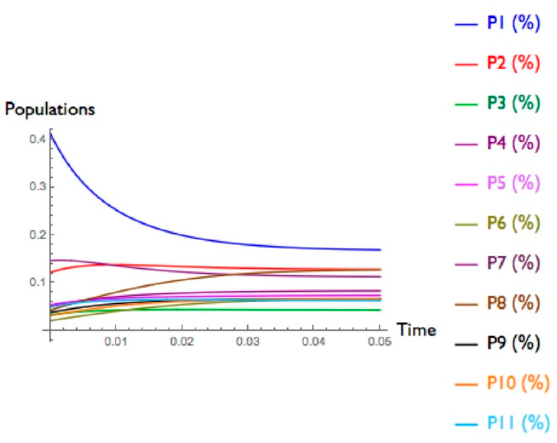
3.3.2. Illustrative Example
4. How Can These Models Contribute for Building Resilient Systems?
- Nature highlights the different essence and characteristics of both dynamic models. On one hand, the Lotka–Volterra are models that aim to explore the dynamic functions of a given environmental system N, whereas the SDM models may be considered as a tool used to study and analyze the model or the system.
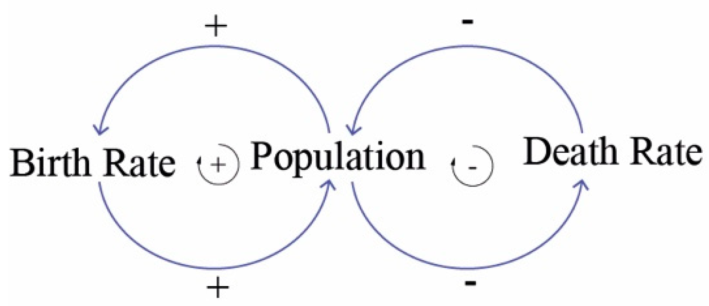
- Input is intended as the modalities to insert and deal with data at different spatial scales, as well as the possibility to integrate the participatory process. Generally, the considered dynamic models allow the insert of only quantitative data and the employment of different spatial scales (from local to regional and superior). As far as the participatory process is concerned in the SDM models, the decision makers may be integrated since the early phases of the process by using causal loops (Figure 1) that facilitate the interpretation of the system functioning and the integration of different stakeholders’ perspectives [14,50]. In the LV models, the participatory process may be integrated only by other evaluation procedures, such as the Multicriteria Analysis (MCA), by using a system of indicators and indices [79,87].
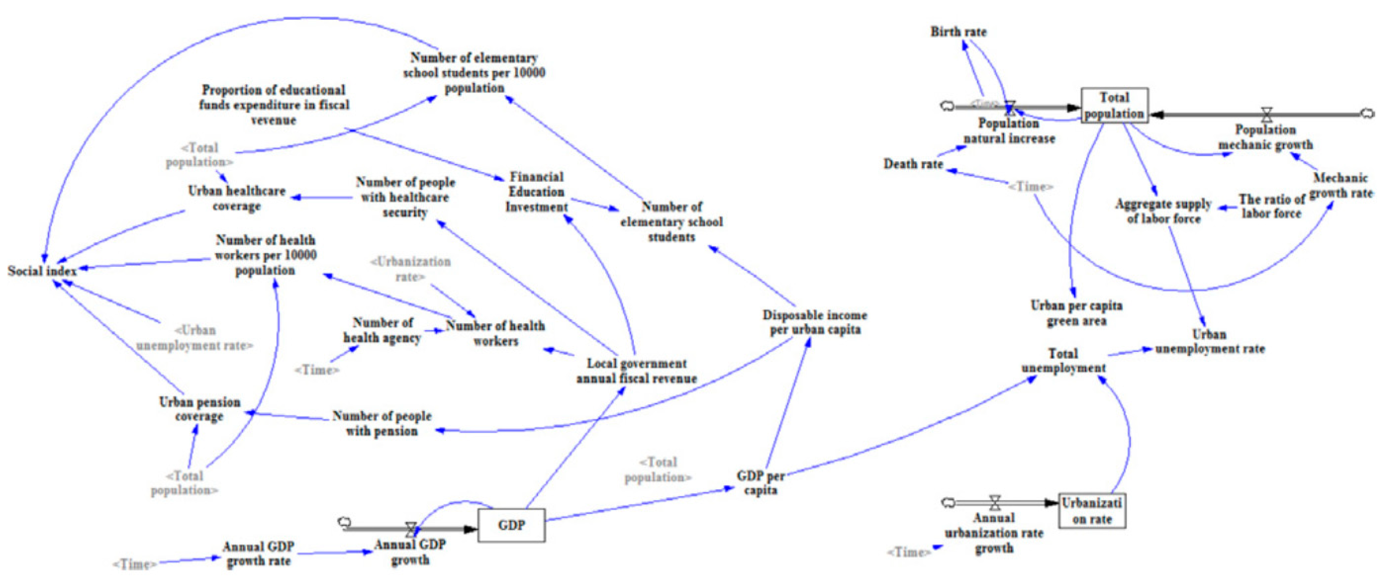
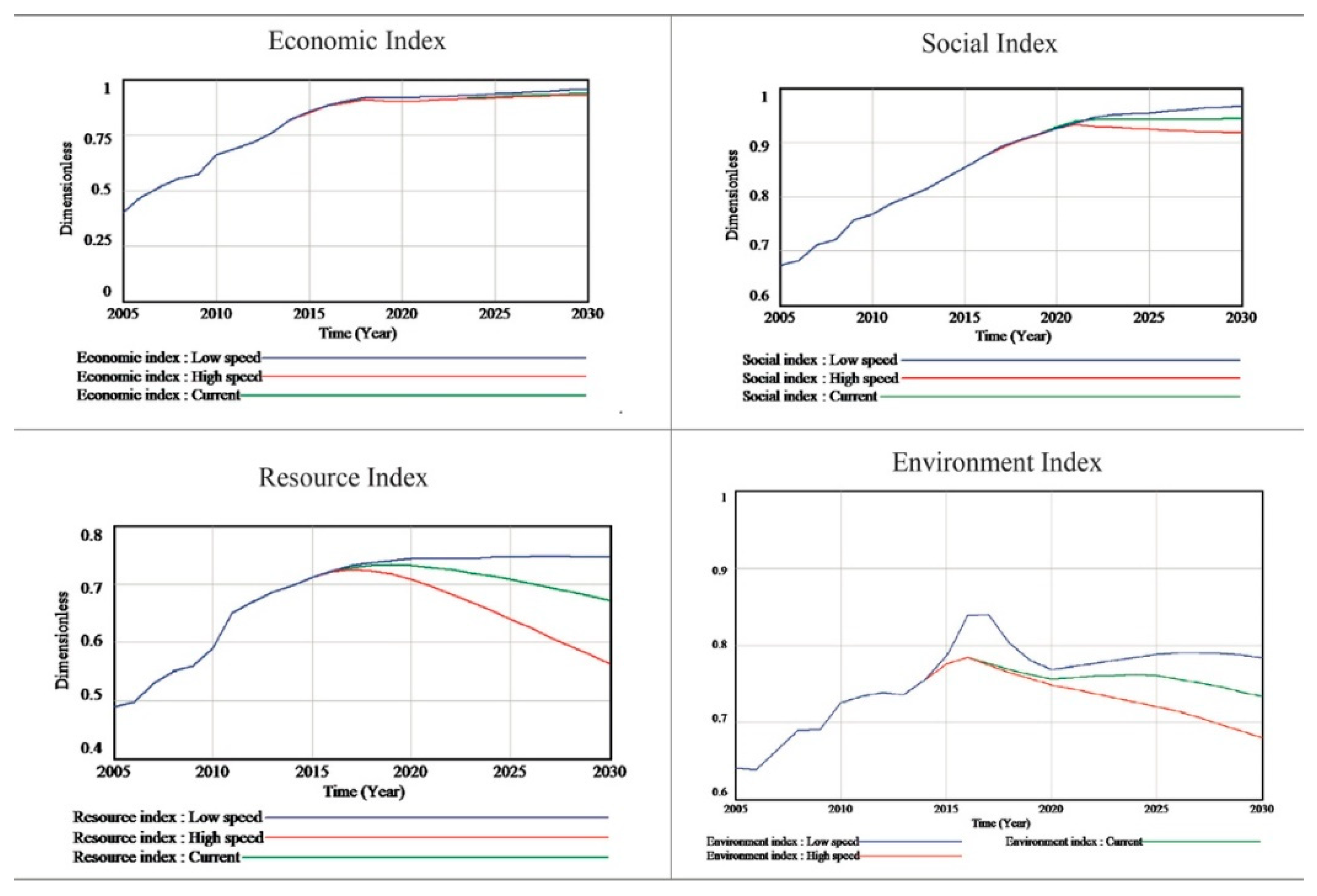
- Output refers to the final result produced through the considered dynamic models, such as the scenario simulation, the use of the time scale, the spatial scale, the graphical representation and the sensitivity analysis with the aim to validate the scenarios produced. Particularly, both SDM and LV models simulate possible future scenarios and these represent, generally, the final output through a graphic plot in that the linear function is represented. Unlike the LV models, the SDM models show, since the initial phase, a graphical representation of the relations between the considered variables and they allow to make, after the scenario simulation, a sensitivity analysis. These two DMs use, in different ways the time scale: the SDM model use a real time scale that may be traduced in months, years or centuries, whereas the LV model uses an arbitrary time scale that may be subdivided in an initial phase when the function starts with the state of art conditions (t0), transitory phase, when the linear function evolves in terms of growth or degrowth, and a final phase, when the linear function became stable. The arbitrary time scale may be traduced in a real time scale by considering the historical series of the analyzed parameters [74]. Sensitivity analysis is a valuable procedure for testing the model response with respect to the variation of parameter values, as well as to identify those parameters that have more impact than the others on the investigated phenomenon [88]. Sensitivity analysis can increase the reliability of the model and thus, reduce the uncertainty of parameters used in the models. A very common sensitivity test is the One-At-Time approach (OAT) [89] that is often used in Multicriteria Analysis as final tuning [75,90,91]. This, in fact, facilitates the scenarios’ assessment when actors and stakeholders are involved in a participatory decision-making process [92,93].
- Software refers to the availability of software and the modalities to solve the Ordinary Differential Equations (ODEs). On one hand, the SDM models are characterized by the use of specific software, such as STELLA, Venism and Powerism, that formulate themselves the ODEs from which the scenarios’ simulations are produced. On the other hand, LV models are generally employed through mathematical software, such as MatLab and Mathematica Software, and these need to write manually the ODEs to obtain the prediction of scenarios (Figure 6). In this sense, both the dynamic models use the ODEs as an output, but in different ways. From the point of view of the availability, both dynamic models may be written through specific packages in open programming languages, such “deSolve” for R, “Simupy” for Python, “Mat Cont for Matlab” and “Nova modeler” for ecological modelling.
- Integration refers to the capability of DMs to integrate different techniques and evaluation methodologies. For instance, the considered dynamic models are a suitable tool to being integrated with Multicriteria Analysis (MCA) [75], as well as with the Agent-Based Models (ABM) [94] and Hedonic Price Model (HPM) [95]. Specifically, MCA can be used at two different phases: (1) at the beginning, to support the problem articulation and the identification of the variables to be included in the model; (2) after the scenarios’ simulation to support the evaluation of the different performances through final score calculation or ranking elaboration. Shafiei et al. [96] integrate SDM and Agent-Based Models to better understand the effects, not only on the system but also on the agent of the transition to sustainable mobility.
- Mapping is intended as the possibility to visualize the scenarios using GIS-based methods and the possibility to interact the dynamic model and the GIS interface through a programming language (e.g., QGIS and Python). Actually, the integration of DMs simulation results into GIS is developed by users in specific plug-ins (e.g., PANDORA 3.0 [97]) or by using specific coding platforms (e.g., QGIS Python console) and to get a spatial visualization of the output. Despite the requirement of specific competences to manage DMs in GIS environment, the users may support decision makers in better interpreting certain dynamics related to urban resilience by visualizing spatially the output of the dynamic model in a final map and therefore, identifying specific policies and solutions.
- Scenario planning refers to the prediction of future scenarios and the definition for each scenario of objectives and strategies. Both SDM and LV models allow to predict the way variables evolve, starting from the state of art conditions (t0) [50]. In this sense, both the SDM and the LV models are useful supports for the decision makers for identifying the most critical areas and adopting specific policies and interventions.
- Scale refers to the application of dynamic models at different scales. Moreover, the SDM considers a system as a whole, analyzing and focusing on its components and sub-components. In fact, SDMs are mostly applied to municipal or metropolitan scales. LV models are generally employed to provincial and sub-regional scales and to those territories with a rural vocation.
5. Conclusions and Future Perspectives
- These DMs are currently considered as some of the most promising models for understanding multi-dimensional problems related to urban and territorial systems.
- If experiments are impossible in the real world, simulations become the main way we can learn effectively about the dynamics of complex systems. Dynamic models are the most appropriate techniques to simulate complex and dynamic systems with the aim of developing policy and learning to effectively manage the system [50,100].
- These models are able to predict the effects of the actions over time on the state of the system. For this reason, both the DMs considered can be applied to evaluate the possible effects of urban and territorial policies in order to enhance urban resilience.
Author Contributions
Funding
Conflicts of Interest
References
- Collins, A. The Global Risks Report 2019 14th Edition Insight Report. 2019. Available online: http://www3.weforum.org/docs/WEF_Global_Risks_Report_2019.pdf (accessed on 16 December 2019).
- Gencer, E.A.; For, A.H.; Government, L. A Handbook for Local Government Leaders Making Cities Resilient—My City is Getting Ready! Making Cities Resilient—My City is Getting Ready! UNISDR: Geneva, Switzerland, 2017. [Google Scholar]
- Bottero, M.; Caprioli, C.; Cotella, G.; Santangelo, M. Sustainable Cities: A Reflection on Potentialities and Limits based on Existing Eco-Districts in Europe. Sustainability 2019, 11, 5794. [Google Scholar] [CrossRef]
- Datola, G.; Bottero, M.; De Angelis, E. How Urban Resilience Can Change Cities: A System Dynamics Model Approach. In Proceedings of the Computational Science and Its Applications—ICCSA 2019; Misra, S., Gervasi, O., Murgante, B., Stankova, E., Korkhov, V., Torre, C., Rocha, A.M.A.C., Taniar, D., Apduhan, B.O., Tarantino, E., Eds.; Springer International Publishing: Cham, Germany, 2019; pp. 108–122. [Google Scholar]
- UNISDR. The Sendai Framework for Disaster Risk Reduction: The Challenge for Science. R. Soc. Meet. Note. 2015. Available online: https://royalsociety.org/~/media/policy/Publications/2015/300715-meeting-note%20-sendai-framework.pdf (accessed on 16 December 2019).
- United Nations. International Strategy for Disaster Reduction Hyogo Framework for Action 2005–2015: Building the Resilience of Nations. 2015. Available online: https://www.unisdr.org/files/1037_hyogoframeworkforactionenglish.pdf (accessed on 16 December 2019).
- Desouza, K.C.; Flanery, T.H. Designing, planning, and managing resilient cities: A conceptual framework. Cities 2013, 35, 89–99. [Google Scholar] [CrossRef]
- Chelleri, L.; Waters, J.J.; Olazabal, M.; Minucci, G. Resilience trade-offs: Addressing multiple scales and temporal aspects of urban resilience. Environ. Urban. 2015, 27, 181–198. [Google Scholar] [CrossRef]
- Sharifi, A.; Yamagata, Y. Resilience-Oriented Urban Planning. In Proceedings of the Lecture Notes in Energy; Springer: Berlin/Heidelberg, Germany, 2018. [Google Scholar]
- Mushir, S. Urban Resilience Planning: A Way to Respond to Uncertainties—Current Approaches and Challenges. In Making Cities Resilient; Springer: Berlin/Heidelberg, Germany, 2019. [Google Scholar]
- Pejic Bach, M.; Tustanovski, E.; Ip, A.W.H.; Yung, K.L.; Roblek, V. System dynamics models for the simulation of sustainable urban development: A review and analysis and the stakeholder perspective. Kybernetes 2019. [Google Scholar] [CrossRef]
- Pagano, A.; Pluchinotta, I.; Giordano, R.; Petrangeli, A.B.; Fratino, U.; Vurro, M. Dealing with Uncertainty in Decision-Making for Drinking Water Supply Systems Exposed to Extreme Events. Water Resour. Manag. 2018, 32, 2131–2145. [Google Scholar] [CrossRef]
- Tan, Y.; Jiao, L.; Shuai, C.; Shen, L. A system dynamics model for simulating urban sustainability performance: A China case study. J. Clean. Prod. 2018, 199, 1107–1115. [Google Scholar] [CrossRef]
- Pluchinotta, I.; Pagano, A.; Giordano, R.; Tsoukiàs, A. A system dynamics model for supporting decision-makers in irrigation water management. J. Environ. Manag. 2018, 223, 815–824. [Google Scholar] [CrossRef]
- Schwarz, N.; Haase, D.; Seppelt, R. Omnipresent sprawl? A review of urban simulation models with respect to urban shrinkage. Environ. Plan. B Plan. Des. 2010, 37, 265–283. [Google Scholar] [CrossRef]
- Coutu, D.L. How resilience works. Harv. Bus. Rev. 2002, 80, 46–56. [Google Scholar]
- Luthans, F.; Vogelgesang, G.R.; Lester, P.B. Developing the Psychological Capital of Resiliency. Hum. Resour. Dev. Rev. 2006, 5, 25–44. [Google Scholar] [CrossRef]
- Holling, C.S. Resilience and Stability. Annu. Rev. Ecol. Syst. 1973, 4, 1–23. [Google Scholar] [CrossRef]
- Fiksel, J. Designing Resilient, Sustainable Systems. Environ. Sci. Technol. 2003, 37, 5330–5339. [Google Scholar] [CrossRef]
- Hollnagel, E.; Woods, D.; Leveson, N. Resilience Engineering: Concepts and Precepts; CRC Press: Boca Raton, FL, USA, 2006. [Google Scholar]
- Carpenter, S.; Walker, B.; Anderies, J.M.; Abel, N. From Metaphor to Measurement: Resilience of What to What? Ecosystems 2001, 4, 765–781. [Google Scholar] [CrossRef]
- Folke, C.; Carpenter, S.; Elmqvist, T.; Gunderson, L.; Holling, C.S.; Walker, B. Resilience and sustainable development: Building adaptive capacity in a world of transformations. AMBIO 2002, 31, 437–441. [Google Scholar] [CrossRef]
- Walker, B.; Holling, C.S.; Carpenter, S.R.; Kinzig, A. Resilience, adaptability and transformability in social-ecological systems. Ecol. Soc. 2004, 9. Available online: https://www.ecologyandsociety.org/vol9/iss2/art5/ (accessed on 16 December 2019). [CrossRef]
- Nelson, D.R.; Adger, W.N.; Brown, K. Adaptation to Environmental Change: Contributions of a Resilience Framework. Annu. Rev. Environ. Resour. 2007, 32, 395–419. [Google Scholar] [CrossRef]
- Tanner, T.; Mitchell, T.; Polack, E.; Guenther, B. Urban Governance for Adaptation: Assessing Climate Change Resilience in Ten Asian Cities. IDS Work. Pap. 2009, 315, 1–47. [Google Scholar] [CrossRef]
- Tyler, S.; Moench, M. A framework for urban climate resilience. Clim. Dev. 2012, 4, 311–326. [Google Scholar] [CrossRef]
- Ahern, J. From fail-safe to safe-to-fail: Sustainability and resilience in the new urban world. Landsc. Urban. Plan. 2011, 100, 341–343. [Google Scholar] [CrossRef]
- Wilkinson, C. Social-ecological resilience: Insights and issues for planning theory. Plan. Theory 2012, 11, 148–169. [Google Scholar] [CrossRef]
- Coaffee, J. Risk, resilience, and environmentally sustainable cities. Energy Policy 2008, 36, 4633–4638. [Google Scholar] [CrossRef]
- Cutter, L.S.; Barnes, L.; Berry, M.; Burton, C.; Evans, E.; Tate, E.; Webb, J.; Carolina, S. Community and Regional Resilience: Perspectives from Hazards, Disasters, and Emergency Management. Geography 2008, 1, 2301–2306. [Google Scholar]
- Gaillard, J.C. Vulnerability, capacity and resilience: Perspectives for climate and development policy. J. Int. Dev. 2010, 22, 218–232. [Google Scholar] [CrossRef]
- Meerow, S.; Newell, J.P.; Stults, M. Defining urban resilience: A review. Landsc. Urban. Plan. 2016, 147, 38–49. [Google Scholar] [CrossRef]
- Godschalk, D.R. Urban Hazard Mitigation: Creating Resilient Cities. Nat. Hazards Rev. 2003, 4, 136–143. [Google Scholar] [CrossRef]
- Batty, M. The size, scale, and shape of cities. Science. 2008, 319, 769–771. [Google Scholar] [CrossRef]
- Klein, R.J.T.; Nicholls, R.J.; Thomalla, F. Resilience to natural hazards: How useful is this concept? Environ. Hazards 2003, 5, 35–45. [Google Scholar] [CrossRef]
- Adger, W.N. Social and ecological resilience: Are they related? Prog. Hum. Geogr. 2000, 24, 347–364. [Google Scholar] [CrossRef]
- Pendall, R.; Foster, K.A.; Cowell, M. Resilience and regions: Building understanding of the metaphor. Cambr. J. Reg. Econ. Soc. 2010, 3, 71–84. [Google Scholar] [CrossRef]
- Sharifi, A.; Yamagata, Y. Principles and criteria for assessing urban energy resilience: A literature review. Renew. Sustain. Energy Rev. 2016, 60, 1654–1677. [Google Scholar] [CrossRef]
- Leichenko, R. Climate change and urban resilience. Curr. Opin. Environ. Sustain. 2011, 3, 164–168. [Google Scholar] [CrossRef]
- Pierce, J.C.; Budd, W.W.; Lovrich, N.P. Resilience and sustainability in US urban areas. Environ. Politic 2011, 20, 566–584. [Google Scholar] [CrossRef]
- Sharifi, A.; Yamagata, Y. Major Principles and Criteria for Development of an Urban Resilience Assessment Index. In Proceedings of the International Conference and Utility Exhibition on Green Energy for Sustainable Development (ICUE), Pattaya City, Thailand, 19–21 March 2014; pp. 1–5. [Google Scholar]
- Holling, C.S. Resilience and Stability of Ecological Systems. Annu. Rev. Ecol. Syst. 2003, 4, 1–23. [Google Scholar] [CrossRef]
- Cutter, S.L.; Barnes, L.; Berry, M.; Burton, C.; Evans, E.; Tate, E.; Webb, J. A place-based model for understanding community resilience to natural disasters. Glob. Environ. Chang. 2008, 18, 598–606. [Google Scholar] [CrossRef]
- Tompkins, E.L.; Amundsen, H. Perceptions of the effectiveness of the United Nations Framework Convention on Climate Change in advancing national action on climate change. Environ. Sci. Policy 2008, 11, 1–3. [Google Scholar] [CrossRef]
- Wang, L.; Xue, X.; Zhang, Y.; Luo, X. Exploring the Emerging Evolution Trends of Urban Resilience Research by Scientometric Analysis. Int. J. Environ. Res. Public Health 2018, 10, 2181. [Google Scholar] [CrossRef]
- Pizzo, B. Problematizing resilience: Implications for planning theory and practice. Cities 2015, 43, 133–140. [Google Scholar] [CrossRef]
- Letcher, R.A.K.; Jakeman, A.J.; Barreteau, O.; Borsuk, M.E.; ElSawah, S.; Hamilton, S.H.; Henriksen, H.J.; Kuikka, S.; Maier, H.R.; Rizzoli, A.E.; et al. Selecting among five common modelling approaches for integrated environmental assessment and management. Environ. Model. Softw. 2013, 47, 159–181. [Google Scholar]
- Neuwirth, C.; Peck, A.; Simonović, S.P. Modeling structural change in spatial system dynamics: A Daisyworld example. Environ. Model. Softw. 2015, 47, 159–181. [Google Scholar] [CrossRef]
- Bala, B.K.; Arshad, F.M.; Noh, K.M. System Dynamics. Modelling and Simulation; Springer: Singapore, 2017; ISBN 978-981-10-2043-8. [Google Scholar]
- Forrester, J.W. Industrial Dynamics; M.I.T. Press: Cambridge, MA, USA, 1964. [Google Scholar]
- Forrester, J.W. Principles of Systems; System Dynamics Series; Productivity Press: Portland, OR, USA, 1990; ISBN 9780915299874. [Google Scholar]
- Thompson, B.P.; Bank, L.C. Use of system dynamics as a decision-making tool in building design and operation. Build. Environ. 2010, 45, 1006–1015. [Google Scholar] [CrossRef]
- Swart, J. A system dynamics approach to predator-prey modeling. Syst. Dyn. Rev. 1990, 6, 94–99. [Google Scholar] [CrossRef]
- Crookes, D.; Blignaut, J. Predator–prey analysis using system dynamics: An application to the steel industry. S. Afr. J. Econ. Manag. Sci. 2016, 19, 733–746. [Google Scholar] [CrossRef]
- Guan, D.; Gao, W.; Su, W.; Li, H.; Hokao, K. Modeling and dynamic assessment of urban economy-resource-environment system with a coupled system dynamics–Geographic information system model. Ecol. Indic. 2011, 11, 1333–1344. [Google Scholar] [CrossRef]
- Güneralp, B.; Seto, K.C. Environmental impacts of urban growth from an integrated dynamic perspective: A case study of Shenzhen, South China. Glob. Environ. Chang. 2008, 18, 720–735. [Google Scholar] [CrossRef]
- Yao, H.; Shen, L.; Tan, Y.; Hao, J. Simulating the impacts of policy scenarios on the sustainability performance of infrastructure projects. Autom. Constr. 2011, 20, 1060–1069. [Google Scholar] [CrossRef]
- Yuan, H.; Chini, A.R.; Lu, Y.; Shen, L. A dynamic model for assessing the effects of management strategies on the reduction of construction and demolition waste. Waste Manag. 2012, 32, 521–531. [Google Scholar] [CrossRef]
- Blumberga, A. System Dynamics for Environmental Engineering Students; Riga Technical University: Rīga, Latvia, 2011; ISBN 9789934819629. [Google Scholar]
- Egilmez, G.; Tatari, O. A dynamic modeling approach to highway sustainability: Strategies to reduce overall impact. Transp. Res. Part A Policy Pract. 2012, 46, 1086–1096. [Google Scholar] [CrossRef]
- Shepherd, S.P. A review of system dynamics models applied in transportation. Transportmetrica B 2014, 2, 83–105. [Google Scholar] [CrossRef]
- Yu, C.; Chen, C.; Lin, C.; Liaw, S. Development of a system dynamics model for sustainable land use management. J. Chin. Inst. Eng. 2003, 26, 607–618. [Google Scholar] [CrossRef]
- Park, M.; Kim, Y.; Lee, H.S.; Han, S.; Hwang, S.; Choi, M.J. Modeling the dynamics of urban development project: Focusing on self-sufficient city development. Math. Comput. Model. 2013, 57, 2082–2093. [Google Scholar] [CrossRef]
- Wu, D.; Ning, S. Dynamic assessment of urban economy-environment-energy system using system dynamics model: A case study in Beijing. Environ. Res. 2018, 164, 70–84. [Google Scholar] [CrossRef]
- Kunc, M.; Mortenson, M.J.; Vidgen, R. A computational literature review of the field of System Dynamics from 1974 to 2017. J. Simul. 2018, 12, 115–127. [Google Scholar] [CrossRef]
- Lotka, A.J. Contribution to the Energetics of Evolution. Proc. Natl. Acad. Sci. USA 2006, 8, 1747. [Google Scholar] [CrossRef]
- Turner, M.G.; Gardner, R.H. Landscape Ecology in Theory and Practice; Springer: New York, NY, USA, 2015; ISBN 978-1-4939-2793-7. [Google Scholar]
- Monaco, R. Introduzione ai Modelli Matematici Nelle Scienze Territoriali/Roberto Monaco, Giorgia Servente; Quaderni di matematica per le scienze applicate 2; Celid: Torino, Italy, 2011; ISBN 978-88-7661-927-4. [Google Scholar]
- Finotto, F.; Monaco, R.; Servente, G. Un modello per la valutazione di energia biologica in un sistema ambientale. Sci. Reg. 2010, 9, 61–84. [Google Scholar]
- Pelorosso, R.; Gobattoni, F.; Menconi, M.E.; Vizzari, M.; Grohmann, D.; Ripa, M.; Leone, A. Landscape development scenario analysis by PANDORA model: An application in Umbria Region (Italy). In Proceedings of the International Conference of Agricultural Engineering CIGR-AgEng2012: Agriculture and Engineering for a Healthier Life, Valencia, Spain, 8–12 July 2012. CIGR-AgEng. [Google Scholar]
- Gobattoni, F.; Groppi, M.; Monaco, R.; Pelorosso, R. New Developments and Results for Mathematical Models in Environment Evaluations. Acta Appl. Math. 2014, 132, 321–331. [Google Scholar] [CrossRef]
- Monaco, R. A mathematical model for territorial integrated evaluation. In Smart Evaluation and Integrated Design in Regional Development; Brunetta, G., Ed.; Ashgate: Farnham, UK, 2015; pp. 97–106. ISBN 9781472445834. [Google Scholar]
- Assumma, V.; Bottero, M.; Monaco, R. Landscape Economic Value for Territorial Scenarios of Change: An Application for the Unesco Site of Langhe, Roero and Monferrato. Procedia Soc. Behav. Sci. 2016, 223, 549–554. [Google Scholar] [CrossRef]
- Assumma, V.; Bottero, M.; Monaco, R. Landscape Economic Attractiveness: An Integrated Methodology for Exploring the Rural Landscapes in Piedmont (Italy). Land 2019, 8, 105. [Google Scholar] [CrossRef]
- Assumma, V.; Bottero, M.; Monaco, R.; Soares, A.J. An integrated evaluation model for shaping future resilient scenarios in multi-pole territorial systems. Environ. Territ. Model. Plan. Des. 2018, 4, 17–24. [Google Scholar]
- Assumma, V.; Bottero, M.; Monaco, R.; Soares, A.J. An integrated evaluation methodology to measure ecological and economic landscape states for territorial transformation scenarios: An application in Piedmont (Italy). Ecol. Indic. 2019, 105, 156–165. [Google Scholar] [CrossRef]
- Monaco, R.; Rabino, G.A. A Stochastic Treatment of a Dynamic Model for an Interacting Cities System. In Mathematical Modelling in Science and Technology; Elsevier: Amsterdam, The Netherlands, 1984. [Google Scholar]
- Bottero, M. Assessing the economic aspects of landscape. In Landscape Indicators: Assessing and Monitoring Landscape Quality; Springer: Dordrecht, The Netherlands, 2011; pp. 167–192. ISBN 9789400703650. [Google Scholar]
- Brunetta, G.; Salizzoni, E.; Bottero, M.; Monaco, R.; Assumma, V. Measuring resilience for territorial enhancement: An experimentation in Trentino. Valori e Valutazioni 2018, 20, 69–78. [Google Scholar]
- Goodwin, R.M. A Growth Cycle. In Essays in Economic Dynamics; Palgrave Macmillan: London, UK, 1982; pp. 165–170. ISBN 978-1-349-05504-3. [Google Scholar]
- Weber, L. A Contribution to Goodwin’s Growth Cycle Model from a System Dynamics Perspective. In Proceedings of the 23rd International System Dynamics Conference, Boston, MA, USA, 17–23 July 2005; pp. 17–21. [Google Scholar]
- Hannon, B.; Ruth, M. Modeling Dynamic Biological Systems. In Modeling Dynamic Biological Systems; Springer: Berlin/Heidelberg, Germany, 2014; pp. 3–28. ISBN 978-3-319-05614-2. [Google Scholar]
- Ford, F.A. Modeling the Environment: An Introduction to System Dynamics Models of Environmental Systems; Environmental Studies; Island Press: Washington, DC, USA, 1999; ISBN 9781559636001. [Google Scholar]
- Dalimov, R.; Gappar, N. Limit Cycle, Trophic Function and the Dynamics of Intersectoral Interaction. Curr. Res. J. Econ. Theory 2010, 2, 32–40. [Google Scholar]
- Ilmola, L. Approaches to Measurement of Urban Resilience. In Urban Resilience; Springer: Berlin/Heidelberg, Germany, 2016. [Google Scholar]
- Saaty, T.L. The Analytic Hierarchy Process; McGraw Hill: New York, NY, USA, 1980; ISBN 0070543712. [Google Scholar]
- Elsawah, S.; Pierce, S.A.; Hamilton, S.H.; van Delden, H.; Haase, D.; Elmahdi, A.; Jakeman, A.J. An overview of the system dynamics process for integrated modelling of socio-ecological systems: Lessons on good modelling practice from five case studies. Environ. Model. Softw. 2017, 93, 127–145. [Google Scholar] [CrossRef]
- Norton, J. An introduction to sensitivity assessment of simulation models. Environ. Model. Softw. 2015, 69, 166–174. [Google Scholar] [CrossRef]
- Bottero, M.; Ferretti, V.; Mondini, G. Calculating composite indicators for sustainability. In The Lecture Notes in Computer Science; Springer: Cham, CH, 2015; pp. 20–35. [Google Scholar]
- Bottero, M.; Datola, G.; Monaco, R. Exploring the resilience of urban systems using fuzzy cognitive maps. In International Conference on Computational Science and Its Applications; Springer: Berlin/Heidelberg, Germany, 2017; pp. 338–353. [Google Scholar]
- Sušnik, J.; Vamvakeridou-Lyroudia, L.; Savic, D.; Kapelan, Z. Integrated System Dynamics Modelling for water scarcity assessment: Case study of the Kairouan region. Sci. Total Environ. 2012, 440, 290–306. [Google Scholar] [CrossRef]
- Becchio, C.; Bottero, M.; Corgnati, S.; Dell’Anna, F. Decision making for sustainable urban energy planning: An integrated evaluation framework of alternative solutions for a NZED (Net Zero-Energy District) in Turin. Land Use Policy 2018, 78, 803–817. [Google Scholar] [CrossRef]
- Caprioli, C.; Bottero, M.; Pellegrini, M. An Agent-Based Model (ABM) for the Evaluation of Energy Redevelopment Interventions at District Scale: An Application for the San Salvario Neighborhood in Turin (Italy). In International Conference on Computational Science and Its Applications; Springer: Berlin/Heidelberg, Germany, 2019; ISBN 9783030243012. [Google Scholar]
- Dell’Anna, F.; Bravi, M.; Marmolejo-Duarte, C.; Bottero, M.C.; Chen, A. EPC Green Premium in Two Different European Climate Zones: A Comparative Study between Barcelona and Turin. Sustainability 2019, 11, 5605. [Google Scholar] [CrossRef]
- Shafiei, E.; Stefansson, H.; Asgeirsson, E.I.; Davidsdottir, B.; Raberto, M. Integrated Agent-based and System Dynamics Modelling for Simulation of Sustainable Mobility. Transp. Rev. 2013, 33, 44–70. [Google Scholar] [CrossRef]
- Pelorosso, R.; Gobattoni, F.; Geri, F.; Leone, A. PANDORA 3.0 plugin: A new biodiversity ecosystem service assessment tool for urban green infrastructure connectivity planning. Ecosyst. Serv. 2017, 26, 476–482. [Google Scholar] [CrossRef]
- Giordano, G.; Altafini, C. Qualitative and quantitative responses to press perturbations in ecological networks. Sci. Rep. 2017, 7, 11378. [Google Scholar] [CrossRef]
- Elmqvist, T.; Andersson, E.; Frantzeskaki, N.; McPhearson, T.; Gaffney, O.; Takeuchi, K.; Folke, C. Sustainability and resilience for transformation in the urban century. Nat. Sustain. 2019, 2, 267–273. [Google Scholar] [CrossRef]
- Jakeman, A.J.; Letcher, R.A.; Norton, J.P. Ten iterative steps in development and evaluation of environmental models. Environ. Model. Softw. 2006, 21, 602–614. [Google Scholar] [CrossRef]
- Luna-Reyes, L.F.; Andersen, D.L. Collecting and analyzing qualitative data for system dynamics: Methods and models. Syst. Dyn. Rev. 2003, 19, 271–296. [Google Scholar] [CrossRef]
- Lane, D.C. Formal theory building for the avalanche game: Explaining counter-intuitive behavior of a complex system using geometrical and human behavioural/physiological effects. Syst. Res. Behav. Sci. 2008, 25, 521–542. [Google Scholar] [CrossRef]
- Hovmand, P.F.; Andersen, D.; Rouwette, E.; Richardson, G.; Rux, K.; Calhoun, A. Group Model-Building ‘Scripts’ as a Collaborative Planning Tool. Syst. Res. Behav. Sci. 2012, 29, 179–193. [Google Scholar] [CrossRef]
- Assumma, V.; Bottero, M.; Datola, G.; Angelis, E.; Monaco, R. Come esplorare la resilienza nei sistemi urbani e territoriali? Una panoramica sui modelli dinamici (How to explore resilience in urban and territorial systems? An overview on dynamic models). In Proceedings of the 40th AISRE Conference, Beyond the crises: Renewal, Reconstruction and Local Development, L’Aquila, Italy, 16–18 September 2019. in press. [Google Scholar]


| Author | Field | Definition of Resilience | Static or Dynamic |
|---|---|---|---|
| Holling, 1973 | Ecology | “The ability of these systems to absorb changes of states variables, driving variables, and parameters, and still persist” (p. 17). | Dynamic |
| Pimm, 1984 | Ecology | “How fast the variables return towards their equilibrium following a perturbation” (p. 322). | Static |
| Carpenter et al., 2001 | Social-ecological systems | “The magnitude of disturbance that can be tolerated before a socioecological system (SES) moves to a different region of state space controlled by a different set of processes” (p. 765). | Dynamic |
| Adger, 2000 | Geography | “The ability of groups or communities to cope with external stresses and disturbances as a result of social, political and environmental change” (p. 347). | Dynamic |
| Rose, 2007 | Economics | “The speed at which an entity or system recovers from a severe shock to achieve a desired state” (p. 384). | Dynamic |
| Fiksel, 2006 | Systems engineering | “The capacity of a system to tolerate disturbances while retaining its structure and function” (p. 16). | Dynamic |
| Zhu and Ruth, 2013 | Industrial ecology | “The ability [for industrial ecosystems] to maintain their defining feature of eco-efficient material and energy flows under disruptions” (p. 74). | Dynamic |
| Zeng and colleagues, 2013 | Networks | “The critical threshold at which a phase transition occurs from normal state to collapse” (p. 12). | Static |
| Ouyang, 2014 | Engineering | “The joint ability of a system to resist (prevent and withstand) any possible hazards, absorb the initial damage, and recover to normal operation” (p. 53). | Static |
| Adger, 2000 | Social resilience | “Ability of groups or communities to cope with external stresses and disturbances as a result of social, political and environmental change” (p. 347). | Static |
| Authors and Year | Definition | Field |
|---|---|---|
| Meerow et al., 2016 | “Urban resilience refers to the ability of an urban system—and all its constituent socio-ecological and socio-technical networks across temporal and spatial scales—to maintain or rapidly return to desired functions in the face of a disturbance, to adapt to change, and to quickly transform systems that limit current or future adaptive capacity” (p. 39). | Academic |
| 100 Resilient City Campaign, 2013 | “Urban resilience is the capacity of individuals, communities, institutions, businesses, and systems within a city to survive, adapt, and grow no matter what kinds of chronic stresses and acute shocks they experience” (p. 10). | Political |
| UN-Habitat | “Urban resilience is the measurable ability of any urban system, with its inhabitants, to maintain continuity through all shocks and stresses, while positively adapting and transforming toward sustainability” (p. 5). | Political |
| Urbact, 2004 | “Urban resilience is the capacity of urban systems, communities, individuals, organisations and businesses to recover, maintain their function and thrive in the aftermath of a shock or a stress, regardless its impact, frequency or magnitude” (p. 6). | Political |
| Desouza and Flanery, 2013 | “Urban resilience is the ability to absorb, adapt and respond to changes in urban systems” (p. 89). | Academic |
| Hamilton, 2009 | “Urban resilience is the ability to recover and continue to provide their main functions of living, commerce, industry, government and social gathering in the face of calamities and other hazards” (p. 109). | Academic |
| Lu and Stead, 2013 | “Urban resilience is the ability of a city to absorb disturbance while maintaining its functions and structures” (p. 200). | Academic |
| Thornbush et al., 2013 | “Urban resilience is a general quality of the city’s social, economic, and natural systems to be sufficiently future-proof” (p. 2). | Academic |
| Leichenko, 2011 | “Urban resilience is the ability to withstand a wide array of shocks and stresses” (p. 164). | Academic |
| Romeo—Lankao and Gnatz, 2013 | “Urban resilience is a capacity of urban populations and systems to endure a wide array of hazards and stresses” (p. 358). | Academic |
| OECD, 2016 | “Resilient cities are cities that have the ability to absorb, recover and prepare for future shocks (economic, environmental, social and institutional). Resilient cities promote sustainable development, well-being and inclusive growth” (p. 3). | Political |
| Resilience Alliance, 2002 | “A resilient city is one that has developed capacities to help absorb future shocks and stresses to its social, economic and technical systems and infrastructures, so as to still be able to maintain essentially the same functions, structures, systems and identity” (p. 4). | Political |
| ICLEI, 2015 | “A resilient city is prepared to absorb and recover from any shocks or stress while maintaining its essential functions, structures and identity as well as adapting and thriving in the face of continual change. Building resilience requires identifying and assessing hazard risks, reducing vulnerability and exposure, and lastly, increasing resistance, adaptive capacity and emergency preparedness!” (p. 1). | Political |
| C40, 2017 | “Cities are the forefront of experiencing a host of climate impacts, including coastal and inland flooding, heat waves, droughts, and wildfire. As a result, there is widespread need for municipal agencies to understand and mitigate climate risks to urban infrastructure and services and the communities they serve” (p. 1). | Political |
| Urban Resilience HUB, 2015 | “The measurable ability of any urban system, with its inhabitants, to maintain continuity through all shocks and stresses, while positively adapting and transforming toward sustainability” (p. 6). | Political |
| UNISDR, 2015 | “The ability of a system, community or society exposed to hazards, to resist, absorb, accommodate, adapt to, transform and recover from its effects in a timely and efficient manner, including through the preservation and restoration of its essential basic structures and functions through risk management” (p. 3). | Political |
| Model | Field of Application | Types of Data | Treatment of Space | Treatment of Time | Uncertainty |
|---|---|---|---|---|---|
| Bayesian networks | Decision-making and management, Social learning, System understanding, Prediction | Qualitative and quantitative | Non-spatial | Non-temporal | Structural learning from data and knowledge is possible |
| Coupled component models | Prediction, Forecasting, System understanding, Decision-making and management | Mainly quantitative but qualitative are possible | Comprehensive set of options | Routine | Comprehensive discrimination tests between alternatives |
| Agent-based models | Social learning, System understanding | Mainly quantitative | Limited | Limited | Comprehensive discrimination tests between alternatives |
| Knowledge-based models | Decision-making and management, Prediction, Forecasting | Qualitative and quantitative | Non-spatial | Usually non- temporal | Comprehensive discrimination tests between alternatives |
| Authors and Year | Territorial Scale | Method | Outcome |
|---|---|---|---|
| Wu et al., 2018 | Metropolitan (Beijing, China) | System Dynamics Model System of urban sustainability indicators GIS (Geographic Information System) | Simulating different urban development scenarios to assess their possible effects both temporally and spatially. The objective is to choose the preferable development strategy. |
| Pagano et al., 2017 | Municipal (L’Aquila, Italy) | System Dynamics Model System of performance criteria | Assessing the evolution of the resilience of a drinking water supply in case of natural disaster. |
| Tan et al., 2018 | Metropolitan (Beijing, China) | System Dynamics Model System of indicators | Evaluating three different urban development scenarios considering their possible impacts over time on social, economic and environmental sectors. |
| Guan et al., 2011 | Metropolitan (Chongqing, China) | System Dynamics Model GIS Analytic hierarchy Process (AHP) System of indicators and indices | Development of an integrated evaluation model to assess four different urban scenarios considering the dynamic evolution of considered indicators in both temporal and spatial dimensions. |
| Park et al., 2013 | Metropolitan (Seoul, Korea) | System Dynamics Model | Quantitative analysis of self-sufficient urban development policies for assessing their impacts over time. |
| Lotka–Volterra Models Applied to Territorial and Urban Planning | |||
|---|---|---|---|
| Authors and Year | Territorial Scale | Method | Outcome |
| Finotto and Monaco, 2010 | Municipal | Stability analysis for predicting the production and the time variation of bioenergy; Analysis of territorial characteristics using the ecological graph | Identification of interventions to guarantee the ecological functions of the environmental system with attention on the reduction of the urban sprawl. |
| Gobattoni et al., 2012, 2014, 2016) | Provincial | PANDORA model | Stability analysis on ecological equilibria as future ecological scenarios. |
| Assumma, Bottero and Monaco, 2016, 2019) | Sub-regional | Lotka–Volterra models; System of indicators and indices | Simulation of the population’s mobility with respect to the economic attractiveness. |
| Assumma, Bottero, Monaco and Soares, 2018 | Supra-Municipal | Lotka–Volterra models; System of indicators and indices | Simulation of the population’s dynamics related to economic attractiveness and ecological states as resilience factor. |
| Monaco, 2015 Monaco and Servente, 2006 | Provincial | Lotka–Volterra models; System of indicators and indices | Customer flow is intended as the attractiveness expressed by a system of Gross Leasable Areas (GLAs) by considering their degree of accessibility. |
| Capello and Faggian, 2002 | Municipal | Lotka–Volterra models of prey–predator type | Urban population, urban rent and production profits are combined for understanding urban dynamics of Italian cities. |
| Lotka–Volterra Models | System Dynamic Models | ||
|---|---|---|---|
| Nature | Essence and characters * |  | |
| Input | Use of qualitative and quantitative data |  | |
| Participatory process | | | |
| Use of different spatial scales | |  | |
| Output | Scenario simulation | | |
| Time scale | | | |
| Spatial scale | | | |
| Graphical representation | | | |
| Sensitivity analysis | | | |
| Software | Availability | | |
| Use of Ordinary Differential Equations | | | |
| Integration | Integration with different techniques and methodologies | | |
| Mapping | GIS visualization | | |
| Interactivity | | | |
| Scenario planning | Definition of objectives and strategies | | |
| Prediction of future scenarios | | | |
| Scale | Multiscale | | |
© 2019 by the authors. Licensee MDPI, Basel, Switzerland. This article is an open access article distributed under the terms and conditions of the Creative Commons Attribution (CC BY) license (http://creativecommons.org/licenses/by/4.0/).
Share and Cite
Assumma, V.; Bottero, M.; Datola, G.; De Angelis, E.; Monaco, R. Dynamic Models for Exploring the Resilience in Territorial Scenarios. Sustainability 2020, 12, 3. https://doi.org/10.3390/su12010003
Assumma V, Bottero M, Datola G, De Angelis E, Monaco R. Dynamic Models for Exploring the Resilience in Territorial Scenarios. Sustainability. 2020; 12(1):3. https://doi.org/10.3390/su12010003
Chicago/Turabian StyleAssumma, Vanessa, Marta Bottero, Giulia Datola, Elena De Angelis, and Roberto Monaco. 2020. "Dynamic Models for Exploring the Resilience in Territorial Scenarios" Sustainability 12, no. 1: 3. https://doi.org/10.3390/su12010003
APA StyleAssumma, V., Bottero, M., Datola, G., De Angelis, E., & Monaco, R. (2020). Dynamic Models for Exploring the Resilience in Territorial Scenarios. Sustainability, 12(1), 3. https://doi.org/10.3390/su12010003