Sustainable Visual Analysis for Bank Non-Performing Loans and Government Debt Distress

Abstract

This article visualizes bank non-performing loans (NPLs) and government debt distress data integration and an outcome classification after the outbreak of European sovereign debt. Linear and functional principal component analysis (FPCA) and biclustering are used to show the clustering pattern of NPLs and government debt for 25 EU and BRICS countries (Brazil, Russia, India, China and South Africa) during the period of 2006 to 2017 through high-dimensional visualizations. The results demonstrate that the government debt markets of EU countries experienced a similar trend in terms of NPLs, with a similar size of NPLs across debt markets. Through visualization, we find that the government debt and NPLs of EU and BRICS countries increased drastically after the crisis, and crisis countries are contagious. However, the impact of the Greek debt crisis is lower for non-crisis countries, because the debt markets of these countries are decoupled from the Greek market. We also find that sovereign debtors in the EU countries have much closer fiscal linkages than BRICS countries. The level of crisis in the EU countries will be higher than that in the BRICS countries if crisis is driven by the common shocks of macroeconomic fundamentals.

1. Introduction

The recent global financial crisis of 2008 and the subsequent European debt crisis of 2009 have forced some members of countries and regions, especially of Eurozone countries, to increase public spending to support the development of their banking systems. Fast-growing balance sheets and declining capital ratios have increased banking risks, resulting in larger-scale and more frequent public intervention after the financial crisis [1]. Moreover, these interventions have strained sovereign states and sometimes threatened their debt sustainability. The European sovereign debt crisis has forced some members of countries and regions, especially of Eurozone countries, to increase public spending to support their banks. Under such severe budgetary pressure, it is difficult for some countries to raise funds to finance increasing debt. Although some economists [2] believe that the crisis is over, the recent financial stagflation in Spain and Portugal re-emphasizes that public finances remain a key issue in the Eurozone. It is generally known that Greece’s government debt has increased substantially over the past few decades, which is associated with an increase in the size of the public sector in many industrial countries. The global financial crisis shows that the problems of a market can quickly have negative spillover effects on financial institutions and countries that are generally not considered to be closely related. It cannot be ignored that these spillover effects may lead to a sudden and sharp rise in the overall risk of the financial system, which is described as systemic risk. The bad assets of a bank affect its capital turnover and restrict the reasonable distribution of social resources. Subsequently, the European sovereign debt crisis has raised concerns about the vulnerability of the debt market and the potential systemic risk of sovereign debt defaults in other European debt markets [3].

In recent years, several studies have examined the spillover effect of the European sovereign debt crisis on the finance system. Gertler and Kiyotaki study how fundamental risks and government credit policies pre-affected the vulnerability of the financial system, and the effect of macro prudential policies aimed at offsetting risk-taking motives [4]. Pagano and Sedunov find that the aggregate systemic risk exposure of financial institutions is positively related to sovereign debt yields in European countries in an episodic manner, and they find evidence of a simultaneous relation between systemic risk exposure and sovereign debt yields [5]. Further studies find that the unconventional action of the Federal Reserve weakens the impact of the monetary policy of the Federal Reserve on the stock indexes of emerging countries [6]. Subsequently, Papadamou et al. use meta-analysis techniques to capture the impact of unconventional monetary policies on key macroeconomic indicators [7]. In a recent study, Morais et al. confirmed that a softening of foreign monetary policy has expanded the credit supply of foreign banks and produced a strong practical effect at the enterprise level. The results support the international risk-taking channels and spillover effects on emerging markets of core countries’ monetary policy, whether in the softening or tightening part of monetary policy [8].

Another strand of the literature is focused on the relation between government debt defaults and financial crises. Government debt defaults spread to the financial system when banks hold large amounts of government debt in their portfolios [9,10]. NPLs in the Greek banking system can be explained mainly by public debt, which relates rising sovereign debt to higher NPLs [11]. Furthermore, all financial systems in Europe have been affected by sovereign debt defaults, and the sovereign debt defaults have exacerbated the risks of the financial system [12]. Makri et al. reveal strong correlations between NPLs and public debt of the Eurozone’s banking systems for the period 2000–2008, and fiscal problems may raise bad loans in this region [13]. Ghosh finds that liquidity risk, greater capitalization, greater cost inefficiency, poor credit quality and banking industry size significantly increase bank non-performing loans [14]. Similarly, inflation, state unemployment rates, and US public debt significantly increase bank non-performing loans. Reboredo and Ugolini find that, before the debt crisis, sovereign debt markets were all coupled, and systemic risk was similar for all countries [3]. However, with the onset of the Greek crisis, debt markets decoupled, and the systemic risk of the countries in crisis (excepting Spain) for the European debt market as a whole decreased, whereas the systemic risk of non-crisis countries increased to a small degree. However, even though government debt and NPLs are important aspects of contagion, which can be quantified as the impact of extreme downward movement of one market on other markets, no study has visualized NPLs and government debt distress data integration and an outcome classification. With recent technological advances, visualization of categorical data by means of statistical methods has attracted considerable interest in recent years because the visualization capabilities of statistical software have increased during this time. This paper attempts to fill this gap, especially in three ways to contribute to the existing literature.

First, linear principal component analysis (PCA) is used to process the NPLs and the government debt, which is proposed by Jiang and Yan [15] and generalized by Bakdi and Bensmail [16]. To capture specific features in the financial market, PCA is used to extract the low-dimensional and efficient feature information. The empirical results show that the training accuracy and efficiency have been improved [17]. Although numerous successful applications have been reported, PCA performs poorly in dealing with nonlinear processes because it characterizes only the linear correlation among variables and does not explore the nonlinear relationships. Several nonlinear monitoring methods have been proposed to deal with the nonlinearity of a process [18,19]. Florackis and Krisztián use nonlinear principal component analysis to study the relation between corporate governance and performance. This method enables the extraction of complex features from highly dimensional datasets [20]. To enhance the overall efficiency of Romanian banks, Stoica et al. apply PCA to classify the banks into different operational strategies groups based on their relative efficiency scores. The results show that very few banks have utilized Internet banking services in their production process to increase their level of efficiency [21]. The research of Jiang and Yan confirms that PCA is successful in stopping the increasing stochastic trend of NPLs, and in bringing stability (stationarity) to the banking system [22].

Second, to obtain the clustering pattern of the time-course data in a given period of time, we employ functional principal component analysis (FPCA) to process the NPLs and the government debt because linear PCA only shows the clustering pattern of the whole data at a certain time [23]. FPCA is a popular statistical analysis technology for financial data because it can capture the direction of variation and reduce the dimensions of data. Some studies demonstrate that FPCA can extract the collective characteristics of the financial system [24,25,26]. Morseletto proposes a framework for the analysis of influential visualizations and defines criteria for studying their visual characteristics. The criteria are applied to two case studies, the “traffic light” and the “planetary boundaries” diagrams [27]. Kim et al. investigate the technological evolution of Apple through high-dimensional visualization by functional data analysis. The results show that the company will be able to understand changes in consumer demand through clustering visualization figures [23].

Lastly, several clustering techniques on time series datasets have been used to identify relevant groupings [28], and a new biclustering algorithm is proposed to extract time series biclusters and apartment price data sets in metropolitan areas [29]. Therefore, we use clustering techniques to find a group of countries that showed a homogeneous pattern of NPLs and government-to-GDP ratio in a certain period in this paper. Huang applies a biclustering algorithm to explore inconsecutive co-movement patterns of different foreign exchange rates across non-consecutive time periods. A detected bicluster demonstrates the co-moving behaviors of a subset of currencies in inconsecutive time periods, indicating that the currencies moved in different manners in some specific time periods [30]. Xue use a biclustering algorithm to find local patterns in the quantized historical data. A Biclustering-Based Intelligent System could find different patterns which contain a subset of technical indicators with different periodic parameters [31].

An attractive approach for studying interdependencies between NPLs and government debt is to cluster them on the basis of characteristics. Under an efficient clustering scheme, we would expect “similar” NPLs or government debt of countries to be grouped into the same cluster. The clusters can provide insight into governments via this segmentation, and they can avoid risk by allocating investments among the NPLs or government debt in different clusters. By using biclustering methods, we can find useful groups which may not be detected by conventional clustering methods. In this context, the main goal of this study is to visualize NPLs and government debt data integration and outcome classification. Therefore, dimensionality reduction is done by linear PCA and FPCA to extract the main feature and clustering pattern from sample data, and then a biclustering method is used to discover biclusters in the sample data.

The organization of this paper is the following: Section 2 introduces the methodologies such as linear PCA, FPCA and biclustering, and it outlines the data. In Section 3, we start with linear PCA to visualize the clustering of the NPLs and government debt, respectively, followed by the visualization of FPCA and biclustering. Finally, in Section 4, concluding remarks are presented.

2. Methodology and Outline of the Data

2.1. Linear Principal Component Analysis

PCA is an effective multivariate statistical analysis technique for reducing the dimension of large data sets with minimal loss of information and for extracting their structural features [32,33]. It transforms a number of correlated variables into a series of linearly uncorrelated variables called principal components by projecting the observation results onto axes to capture the maximum amount of variability in the original data. The first principal component explains the variability of the original data as much as possible, and each subsequent component explains the remaining variability as much as possible. PCA is optimal from the perspective of minimizing the square distance between the observed values in the input space and the mapped values in the low-dimensional subspace [34].

Given an input data matrix $\mathrm{X}m\times n$, which consists of the centralized sample data ${\left\{xi\right\}}_{i=1}^m$, where $xi\in {\mathrm{R}}^n$, suppose that the matrix $\mathrm{X}$ is decomposed in the following form:

$$\mathrm{X}={\mathrm{TU}}^T={\displaystyle \sum _{i=1}^n{\mathrm{t}}_{\mathrm{t}}{\mathrm{u}}_i^T}$$

(1)

where $\mathrm{T}$ is the scores matrix, $\mathrm{u}i$ is the loading matrix and $\mathrm{U}$ presents an orthogonal matrix of $n\times n$ that can be obtained by dividing the covariance matrix of $\mathrm{X}$ in the form of ${\displaystyle \sum =\mathrm{U}\Lambda {\mathrm{U}}^T}$. Here, $\Lambda$ is a diagonal matrix of eigenvalues $\lambda i$, and the eigenvectors linked with higher eigenvalues are the main components of the data matrix, which correspond to the most variable dimension in the data. This method allows orthogonal transformation to be performed by keeping only the principal component $d(\le n)$, which is called the number of factors [35]. Furthermore, the final matrix will be rewritten without losing significant information if we choose the first $d$ eigenvectors in the form of:

$$\mathrm{X}={\mathrm{T}}_d{\mathrm{T}}_d^T+\mathrm{E}={\displaystyle \sum _{i=1}^d{\mathrm{t}}_i{\mathrm{u}}_i^T+\mathrm{E}}$$

(2)

where $\mathrm{E}$ is the residual matrix produced by $d$. A linear translation of the coefficients is such that the difference between the original data and the reconstructed data is negligible if the feature transformation is applied to the data set and then inverted. The primary task of PCA is to find the eigenvalues and eigenvectors of the sample covariance matrix $\mathrm{C}$:

$$\mathrm{C}=\frac{1}{n}{\displaystyle \sum _{i=1}^{n}xi}{x}_i^T.$$

(3)

Then, we can calculate the eigenvalue $\lambda i$ from the sample covariance matrix $\mathrm{C}$ in the term of

$$\lambda iui=\mathrm{C}uii=1,2,\dots ,n$$

(4)

where $ui$ is the eigenvector corresponding to the eigenvalue $\lambda i$. When only the previous $p$ eigenvectors (corresponding to the eigenvectors arranged in descending order) are used, we can obtain the matrix $\mathrm{S}=U^T\mathrm{X}$; thus the new component $si(i=1,2,\dots ,p)$ is the principal component. Moreover, the eigenvector corresponding to the largest eigenvalue is the direction of the largest variance data distribution. Then, the variance of the data points to the eigenvector along the direction of the second principal component, which corresponds to the eigenvector with the second largest variation, and this eigenvector is orthogonal to the first eigenvector [36]. We use the non-overlapped coherent-values biclusters proposed by Cheng and Church [37] in this paper.

2.2. Functional Principal Component Analysis

Functional principal component analysis (FPCA) is an effective statistical method to extract variance components from multilevel functional data because nonlinear eigenfunctions are used [23]. It can be argued that FPCA provides a more informative method to examine the covariance structure of samples than PCA. Furthermore, FPCA is a more suitable clustering technique for the time-course data in a given period of time.

A common method to realize FPCA is to approximate each original time series of dimension $d$ with $k$ basis functions. Given a series of identically distributed random functions $X_1,\dots ,X_n$, let $y_i(t_j)=x_i(t_j)+e_i(t_j)$ be the observations made at time points $t_i{}_j$, where $y_i(t_j)$ is the random variable, $x_i(t_j)$ is the underlying smooth function that generates the data and $e_i(t_j)$ denotes the unobserved error components. Formally, a functional form of $x_i(t)$ is derived from the sum of weighted basis functions ${\varphi }_k(t)$ as:

$$x_i(t)={\displaystyle \sum _{k=1}^K{c}_{ik}{\varphi }_k(t)}$$

(5)

where $K$ is a set of basis functions (Kim et al., 2018). In order to obtain a smoothing function that fits well with the observed time series, $y_i(t_j)$, we follow the smoothing criteria as:

$$SSE(y|c)={{\displaystyle \sum _{i=1}^n{\displaystyle \sum _{j=1}^T\left[y_i(t_j)-{\displaystyle \sum _{i=1}^K{c}_i{}_k{\varphi }_k(t_j)}\right]}}}^2=(y-\Phi c{)}^{\prime }(y-\Phi c)$$

(6)

where $\Phi$ is a matrix $K\times T$, with ${\Phi }_{kj}={\varphi }_k(t_j)$ [38].

2.3. Biclustering

Biclustering is a powerful technique of data mining that was proposed by Hartigan in 1972, and it has been extensively applied in financial forecasting and trading, market data analysis, information retrieval and other interesting fields. Biclustering can simultaneously find subsets of dimensions’ entities of a data matrix so that the selected entities are consistent in the selected dimension. However, traditional clustering methods only find homogeneous object or attribute groups. Thus, the concept of points and dimensions of biclustering is more uniform, which is very different from clustering. We can find useful groups that traditional clustering methods may not be able to detect by using the biclustering method.

According to the data type, biclusters can be divided into categorical and continuous value types. The data in this paper are continuous value type. Thus, the element values of the $i$th object and the $j$th attribute of the continuous value type bicluster are given by:

$$Bij=\mu +\alpha i+\beta j+\epsilon ij$$

(7)

or they can be modeled as a multiplicative model

$$Bij=\mu \times \alpha i\times \beta j\times \epsilon ij$$

(8)

where $Bij$ is the value of the $i$-th object in the $j$-th attribute; $\mu$ is the overall mean in a bicluster; $\alpha i$ and $Bi$ represent the effects for the $i$th object and the $j$th attribute, respectively, and $\epsilon ij$ denotes the random error (see Lee et al., 2010). Since the multiplicative model can be transformed into an additive model by logarithmic transformation, this paper only deals with the additive model.

2.4. Variables and Data Description

Economic and financial crises can reduce the growth rate while promoting an increase of government debt, as Reinhart and Rogoff analyzed in the post-World War II financial crisis [9]. The financial crisis of 2008 dramatically increased the ratio of sovereign debt to GDP in the Eurozone and other countries and regions. Debt financing became a problem for governments in many countries, sparking doubts about the sustainability of debt in some countries and the survival of the monetary supervision system. Thus, the public debt in countries around the world is under considerable pressure, which is confirmed by the European debt crisis of 2009 that broke out in Eurozone countries.

After 2008, both the government gross debt ratio and the government deficit ratio of the Eurozone countries increased rapidly, which has had a negative impact on long-term fiscal sustainability. It is generally known that Greece has been running a deficit for the past ten years, leading to general government gross debt that became close to 178.6% of the GDP in 2017 (Eurostat, 2017). In this context, we use the general government gross debt to GDP ratio (government-to-GDP ratio) as a substitution variable for government debt distress.

In this paper, we mainly focus on the relation between government debt distress and NPLs. The data are comprised of bank non-performing loan ratios and government-to-GDP ratios, which are retrieved from Eurostat and the International Monetary Fund (IMF). Due to data availability problems in some countries such as Luxembourg, the Netherlands and Finland, we exclude these countries in the sample. The final sample consists of 25 countries from the European Union and the 5 BRICS countries. These 30 countries include developed countries and developing countries, and they also include countries with debt crises and countries without debt crises. Therefore, the sample can represent the global market. The sample spans the period from 1 January 2006 to 30 December 2017, and the period covers the global financial crisis of 2008 and the European sovereign debt crisis of 2009, thus providing a valuable opportunity to study the dependence between NPLs and government debt.

3. Results and Discussion

3.1. Linear PCA for Visualization of NPLs and Government Debt

As the first data analysis, linear PCA is used to process the NPLs ratio and the government-to-GDP ratio of 30 sample countries. In particular, the linear PCA variance proportion and cumulative variance proportion results of 30 countries’ NPLs are shown in

Table 1. Linear principal component analysis (PCA) component variance proportion results of 30 countries’ non-performing loans (NPLs).

	First Component (PC1)	Second Component (PC2)	Third Component (PC3)
Variance proportion (VP)	53.07%	23.73%	12.64%
Cumulative VP	53.07%	76.79%	89.43%

, corresponding to NPLs classification. Each principal component represents its percentage contribution to the whole density variation. The ranking of the principal components explains the density variation based on the corresponding contribution of each factor. It can be seen that the dimensions of NPLs characteristic data are dropped to three dimensions. In particular, the first dominant principal component (PC1) accounts for 53.07%, the second principal component (PC2) explains another 23.73% of variability and the third principal component (PC3) explains 12.64% of the whole variance proportion for FPCA. The variance contribution rate of the first three principal components together account for 89.43% of the whole variability (to take the cumulative proportion that is more than 85%). The results show that the first three principal components reflect 89.43% of the total information in the original index, and the data characteristics of the NPLs ratio can be well described by the first three principal components, which has a good extraction effect.

Similarly, the linear PCA variance proportion and cumulative variance proportion results of 30 sample countries in government-to-GDP ratios explained by the components are shown in

Table 2. Linear PCA component variance proportion results of 30 countries’ government-to-GDP ratio.

	First Component (PC1)	Second Component (PC2)	Third Component (PC3)
Variance proportion (VP)	72.67%	18.21%	4.56%
Cumulative VP	72.67%	90.88%	95.44%

. The first dominant principal component (PC1) accounts for 72.67%, the second principal component (PC2) explains 18.21%, and the third principal component (PC3) explains 4.56% of the whole variance proportion for FPCA. The first three principal components account for 95.44% of the whole variability, and the cumulative variance contribution rate is above 95%. The results show that the first three principal components reflect 95.44% of the total information in the original index, and the data characteristics of the government-to-GDP ratio can be well described by the first three principal components.

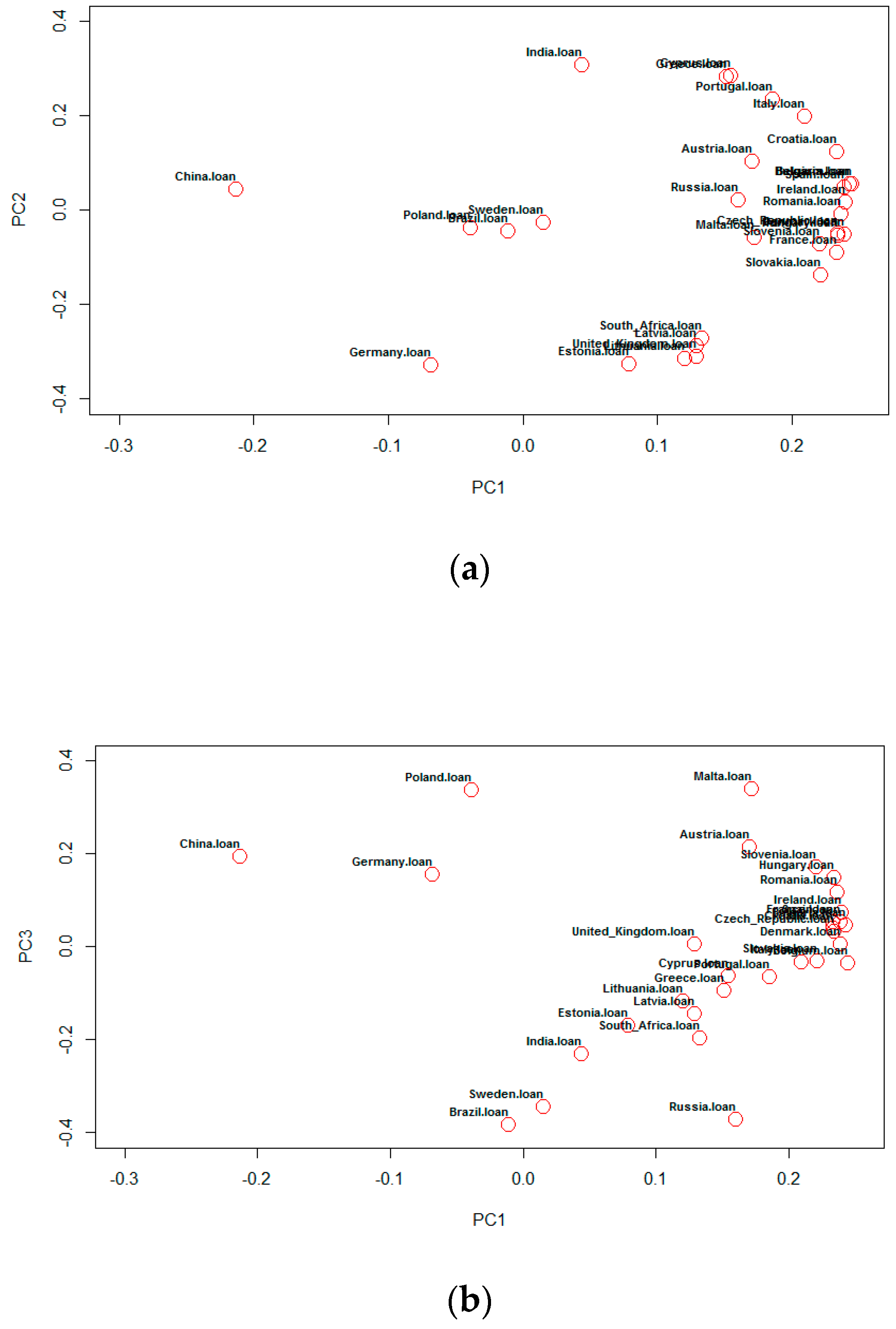
According to the principle of PCA, it is clear that the principal component is a linear combination of the original NPLs (or government-to-GDP ratio) data. Figure 1a–c shows the two-dimensional scatter plots of the 30 countries’ bank NPLs data in the first three principal component (PC1, PC2 and PC3) plane, the position of each country is represented by a red circle. The classification results of NPLs for different countries can be seen from the plane view.

The scatter plot in Figure 1a shows that on the upper half of the horseshoe, there are more sample countries with higher NPLs, although the situation is different in some countries, such as China, India, Brazil, Poland, Germany, Sweden, South Africa and so on. Distinctions between the debt levels of these countries are mainly reflected by PC1. For the lower horseshoe half, it can be stated that PC1 reflects differences in lower bank NPLs. From the classification results in Figure 1b, it can be seen that most countries have come together, but some are very scattered. 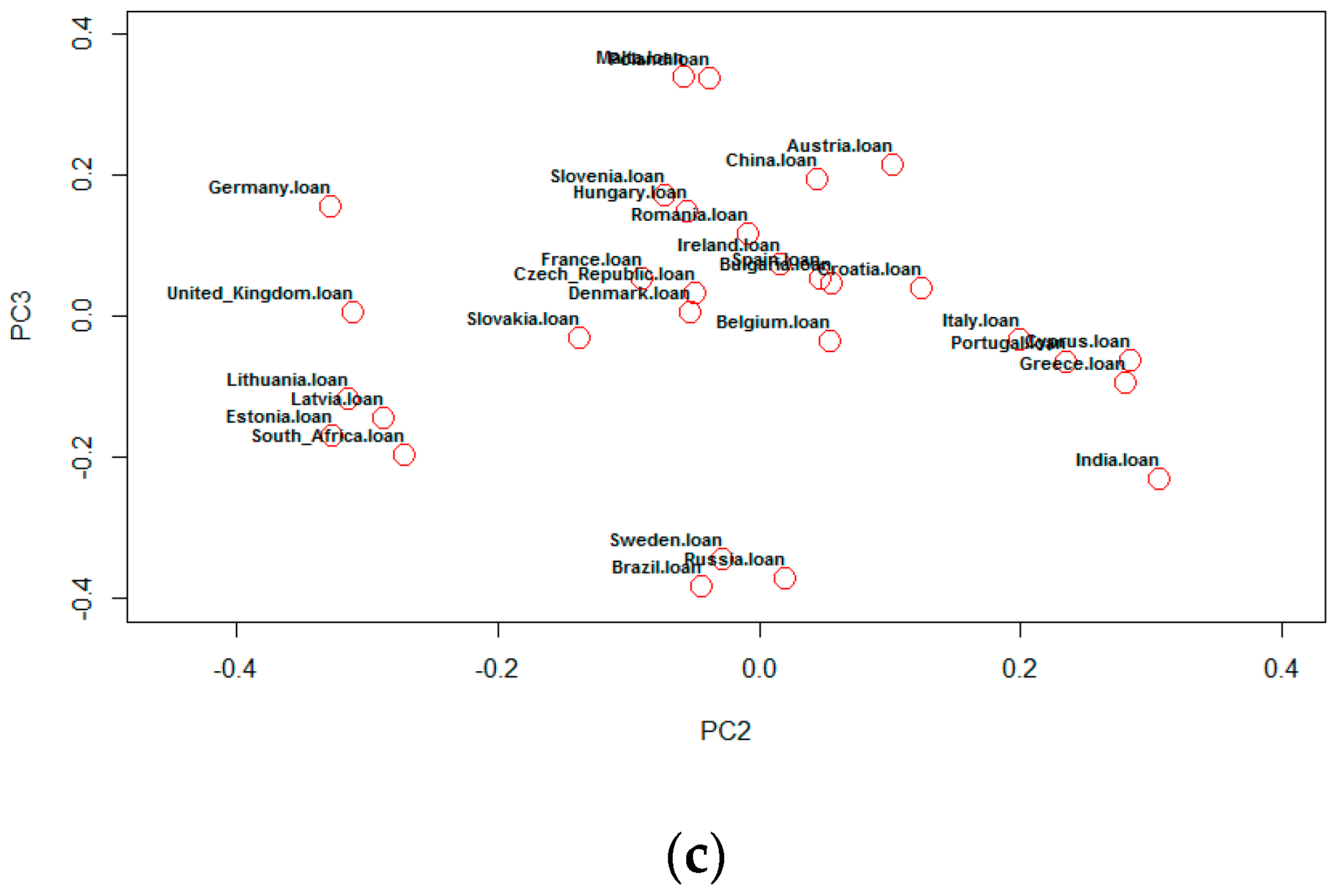The distribution noticeably changed in Figure 1c, where the position of each country is very scattered. However, there is a characteristic of agglomeration. To seek more detailed visualization, a 3-dimensional linear PCA plot of NPLs with the first three principal components is shown in Figure 2.

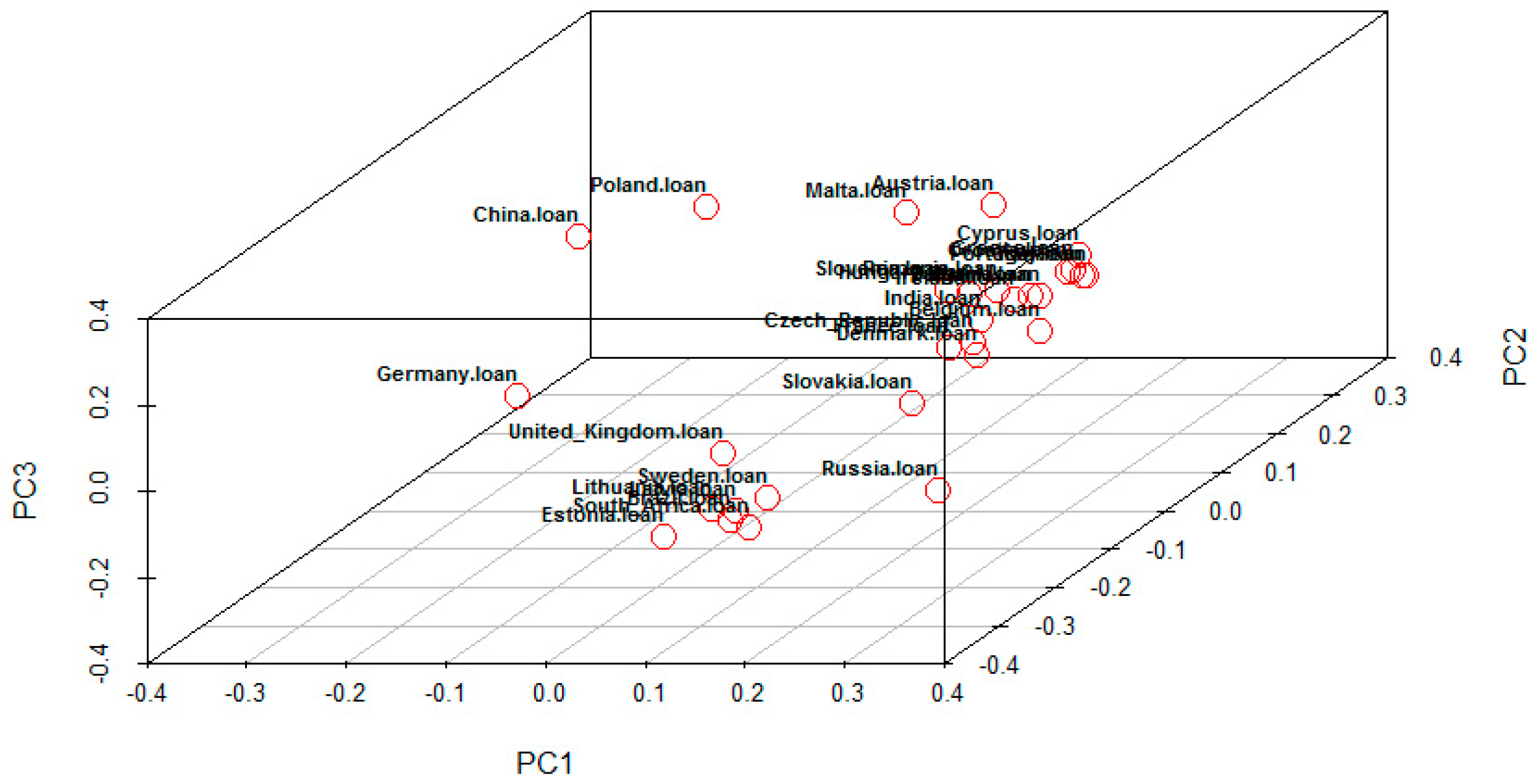
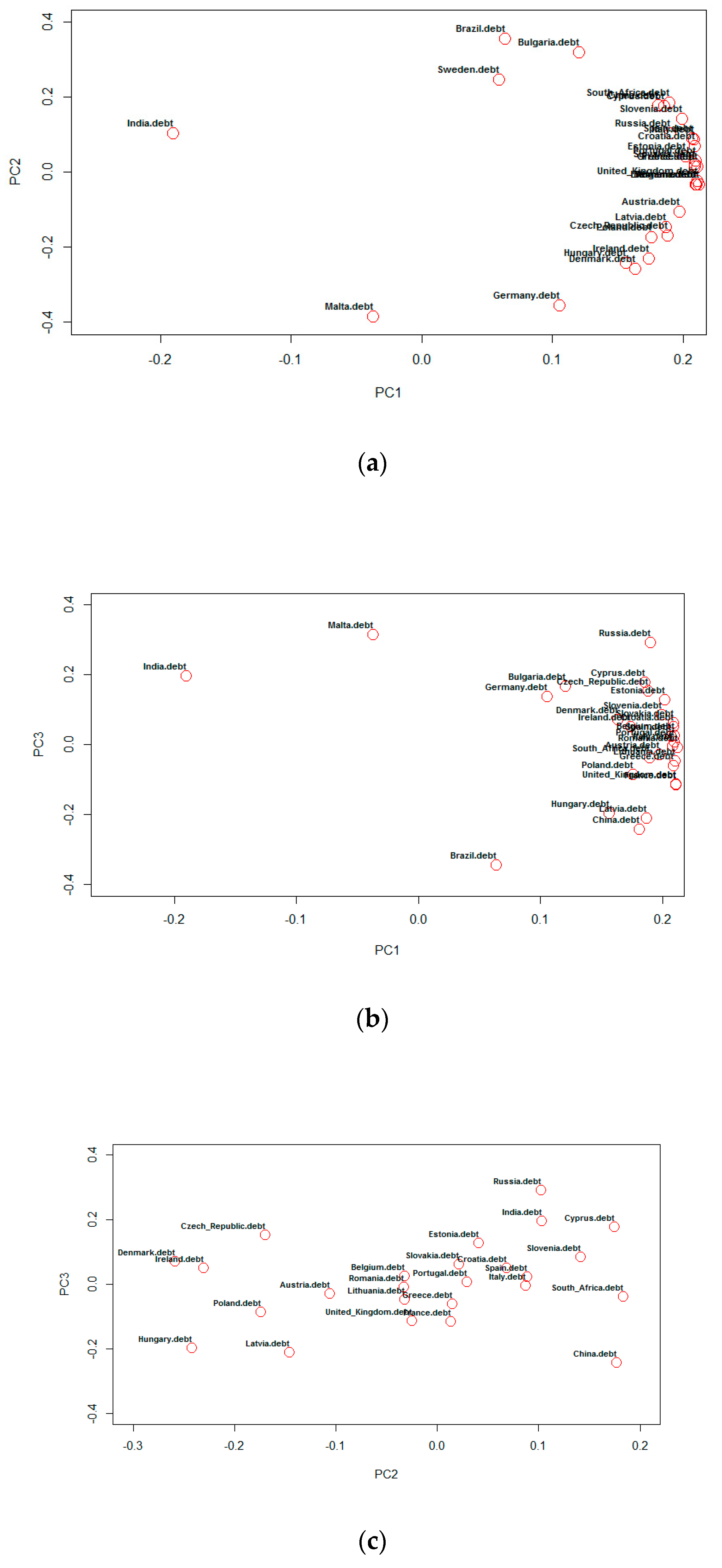
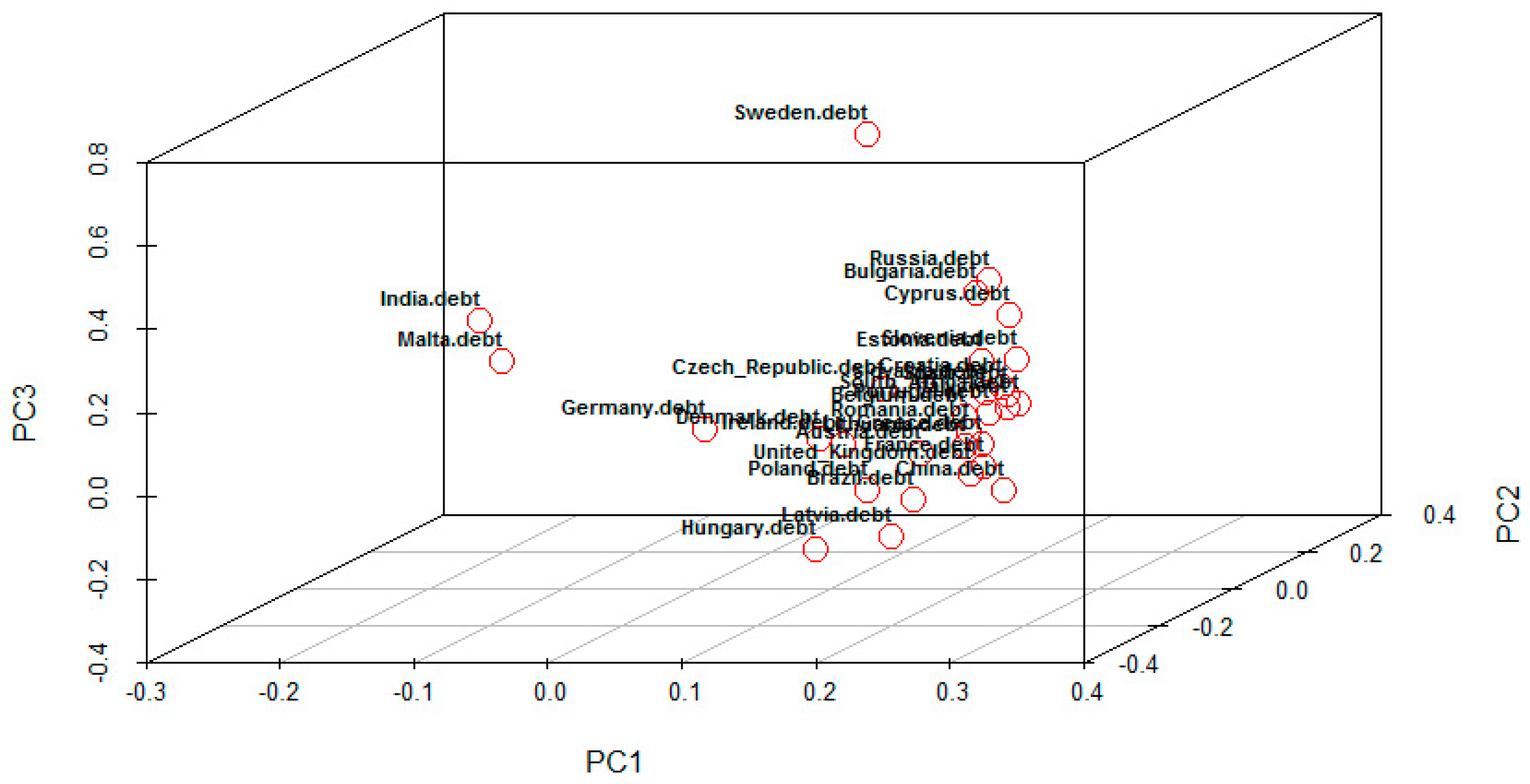
Subsequently, we applied the same method to the government-to-GDP ratio data, and the results are demonstrated in Figure 3a–c. These figures are the scatter plots of the 30 countries’ government-to-GDP data in the principal component (PC1, PC2 and PC3) plane.

The scatter plots in Figure 3a,b show that on the upper half of the horseshoe, there are more sample countries with higher debt, although the situation is different in some countries, such as India, Brazil, Malta, Sweden, Bulgaria and Germany. Distinctions between the debt levels of these countries are mainly reflected by PC1. For the lower horseshoe half, it can be stated that both PC1 and PC2 reflect differences in lower debt. The distribution changed noticeably in Figure 3c, where the position of each country is very scattered. It shows that there is a very small although difference between PC2 and PC3. Figure 4 displays this solution in the PC1–PC2–PC3 space.

It is impossible to obtain the clustering pattern of the time-course data in a given period of time because linear PCA only shows the clustering pattern of the whole data at a certain time [23]. Thus, using the principal components extracted from PCA, it is difficult to obtain very satisfactory results. For example, the cumulative variance contribution rate of the first and second principal components in Table 1 only reaches 76.79%. Meanwhile, it can also be found that the classification effect is not good from Figure 1c and Figure 3c. Therefore, it is necessary to use more effective and accurate feature extraction methods to extract more clustering patterns between data.

3.2. Functional PCA for Visualization of NPLs and Government Debt

The key part of FPCA is to decompose the density change into a set of orthogonal principal component functions that maximize the variance of each component [23]. Therefore, a nonparametric method is used to estimate the return density function in this paper, and then the common structure is extracted from the estimated function. Moreover, given the function of Equation (5), we utilize a Fourier basis to express the smoothing function as a basis function. More particularly, we have $K$ = 5 and $T$ = 12 in Equation (6). Hence, the functional forms of the Fourier series are ${\varphi }_1(t)=1$, ${\varphi }_2(t)=\sin (wt)$, ${\varphi }_3(t)=\cot (wt)$, ${\varphi }_4(t)=\sin (2wt)$ and ${\varphi }_5(t)=\cos (2wt)$. Here, the parameter $w$ is $2\pi /T$ [39].

The roughness penalty is defined by constructing a functional parameter object that consists of a basis object, a derivative order and a smoothing parameter. Subsequently, the function fdPar in R software was used to construct the objects in this paper. We consider the compound fitting criterion as presented in Equation (9):

$$F(c)={\displaystyle \sum _j{\left[y_j-x(t_j)\right]}^2}+\lambda \int {\left[D^{2}x(t)\right]}^{2}dt$$

(9)

where $x(t)=c^{\prime }\varphi (t)$, and $\varphi (t)$ presents a basis function. The smoothing parameter $\lambda$ can balance fitting data, and $\left[D^{2}x(t)\right]$ denotes the curvature of function $x$ at argument value $t$.

Then, a minimizing smoothing criterion is applied to estimate the vector of coefficients $c$. In particular, the generalized cross-validation (GCV) can be computed as:

$$GCV(\lambda )=\left(\frac{n}{n-df(\lambda )}\right)\left(\frac{SSE}{n-df(\lambda )}\right)$$

(10)

where $df(\lambda )$ is a measure of the effective degrees of freedom of the fit defined by smoothing parameter $\lambda$, and the best value for $\lambda$ is the one that minimizes the criterion [40]. Therefore, by using sample data, we calculate a smoothing parameter of $\lambda$ = 101.877. Considering the estimates $\widehat{\mathrm{c}}$, we can obtain the smoothed time series $\widehat{\mathrm{y}}=\Phi \widehat{\mathrm{c}}$ in Equation (6).

After obtaining ${\widehat{y}}_i(t)$, the next step is to find a set of orthogonal functions ${\psi }_j(t)$ that are defined as [38,41]:

$$\langle {\psi }_j(t),{\psi }_k(t)\rangle =\int {\psi }_j(t){\psi }_k(t)dt=0\mathrm{for}\mathrm{all}j\ne k;$$

(11)

$${\Vert {\psi }_j(t)\Vert }^2=\langle {\psi }_j(t),{\psi }_k(t)\rangle =1$$

(12)

For instance, ${\psi }_1(t)$ can be computed by maximizing the objective function in Equation (13):

$${{\displaystyle \sum _i\left(\langle {\widehat{y}}_i(t),{\psi }_1(t)\rangle \right)}}^2={{\displaystyle \sum _i\left(\int {\widehat{y}}_i(t){\psi }_1(t)dt\right)}}^2.$$

(13)

This function is restricted by the constraint ${\Vert {\psi }_1(t)\Vert }^2=1$. At the same time, the function ${\psi }_1(t)$ is also the first principal component. There is no variation left in the time series after ${\psi }_3(t)$ in this study.

Table 3. Functional principal component analysis (FPCA) component variance proportion results of 30 countries’ NPLs.

	First Component (PC1)	Second Component (PC2)	Third Component (PC3)
Variance proportion (VP)	53.1%	46.84%	0.03%
Cumulative VP	53.1%	99.94%	99.97%

shows the proportions of variance proportion and cumulative variance proportion results in NPLs ratio explained by the components. Similar to the PCA method, every principal component represents its percentage contribution to the overall density change. Specifically, the first dominant principal component (PC1) accounts for 53.1%, the second principal component (PC2) explains 46.84%, and the third principal component (PC3) explains 0.03% of the whole variance proportion for FPCA. It is clear that the first three principal components account for 99.97% of the whole variability (to take the cumulative proportion that is more than 99%), which is close to 100%. The results demonstrate that the first three principal components reflect 99.97% of the total information in the original index, and data characteristics of the NPLs ratio can be well described by the first three principal components. In addition, comparing Table 1 and Table 3, it is found that two kinds of the variance contribution rate of the first three principal components obtained by FPCA and PCA differ in nearly 10% points, and the variance contribution rate of the first three principal components obtained by FPCA is significantly higher than PCA. From the above analysis, it can be found that the first three principal components obtained by FPCA have a good dimensionality reduction effect, and the first three principal components contain more data information.

Similarly, the proportions of variance proportion and cumulative variance proportion results of total variation in the government-to-GDP ratio explained by the components are shown in

Table 4. FPCA component variance proportion results of 30 countries’ government-to-GDP ratio.

	First Component (PC1)	Second Component (PC2)	Third Component (PC3)
Variance proportion (VP)	61.75%	38.2%	0.02%
Cumulative VP	61.75%	99.95%	99.99%

. Specifically, the first dominant principal component (PC1 or Harmonic I) accounts for 61.75%, the second principal component (PC2 or Harmonic II) explains 38.2%, and the third principal component (PC3 or Harmonic III) explains 0.02% of the whole variance proportion for FPCA. From Table 4, it can be found that the effect of using FPCA for data dimensionality reduction is obvious; the first three principal components account for 99.99% of the whole variability (to take the cumulative proportion that is more than 99%), which is close to 100%. The results demonstrate that the first three principal components reflect 99.99% of the total information in the original index, and data characteristics of the government-to-GDP ratio can be well described by the first three principal components. In addition, a comparison of Table 2 and Table 4 shows that the effect of the first three principal components obtained by FPCA is significantly better than the results obtained by PCA.

A 2-dimensional scatter plot of the 30 countries’ NPLs data in the first two principal component planes by using FPCA is shown in Figure 5. We use the values provided by the principal components to describe the results in the scatter plot.

The 2D FPCA plot can capture a view of the clusters among NPLs. Through visualizations, we show the relationship of NPLs among the 30 countries. Subsequently, we classified those countries into four groups in

Table 5. NPLs classification of the 30 countries.

Group	Country
Group 1	Bulgaria, Croatia, Malta, Romania, Spain, Slovenia, Belgium, France, Ireland, Austria, Czech Republic, Hungary, Denmark
Group 2	Italy, Cyprus, Portugal, Greece, India
Group 3	Poland, Germany, Sweden, Russia, Brazil, China
Group 4	United Kingdom, Slovakia, Lithuania, Latvia, Estonia, South Africa

based on Figure 5.

The NPLs classifications of Group 1, Group 2, Group 3 and Group 4 in Table 5 correspond to the first, second, third and fourth quadrants in Figure 5, one by one. From the classification results of Table 5, we know that EU countries located in the same region are mostly grouped in the same group. For example, the four countries in Group 2 are located in Southern Europe except for India, and the NPLs in those countries’ banks are so high that the stability of the banking system would be threatened. Non-performing loans and low profit margins are seen as one of the largest problems facing European banks. Due to the threat of crisis in the region, non-performing loans are concentrated in economies, such as Italy, that have underperformed in the past decade. In Italy, 17% of bank loans are bad loans, almost 10 times that of the United States. Even in the worst stage of the financial crisis in 2008–2009, the non-performing loan ratio of the US banking industry was only 5%. Italian banks account for about half of the total non-performing loans of listed banks in the euro area. The non-performing loan ratio of Greek banks is 18.5% at the end of the first quarter of 2012, and this figure does not include the huge loan exposure of banks to the Greek government. Greece’s banks lent 16 billion euros to the government and held 24 billion euros in government bonds, which are bound to default if official Greek creditors refuse to extend more aid. Data from the Central Bank of Portugal recently showed that the non-performing loans from banks to the private sector and households had been on the rise, reaching 14.37 billion euros by June 2012, accounting for 5.82% of the total loans from private enterprises and households, 52% of which belonged to the housing, construction and real estate industries.

The countries of Group 2 have experienced serious debt crisis, except India, and the banking system industry has been greatly impacted. Some of the countries in Group 1 have had debt crises, some have not, but banks have a large number of non-performing loans is their common feature. Consistent with Group 1, the scale of non-performing loans in these countries in Group 2 is also very large, but it is smaller than that in the Group 1, and the banks in these countries are more vulnerable in the economic recession. Most South and Western European countries are in Group 1, and these countries also face high NPLs. In addition, the NPLs of the countries in Group 3 and Group 4 are slightly better than in the previous countries, suggesting that the assets and risk-bearing capacity of banks in Central European, Northern European, Eastern European and BRICS countries are in good condition. In addition, in order to capture the detailed visualization, a 3-dimensional FPCA plot of NPLs with the first three principal components is provided in Figure 6. The spots in the figure show obvious clusters of NPLs data in the 30 countries, implying that those time series data move together over the sample period.

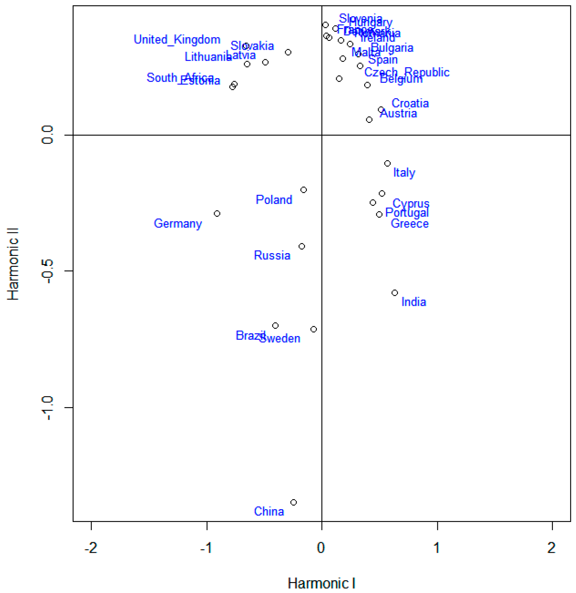
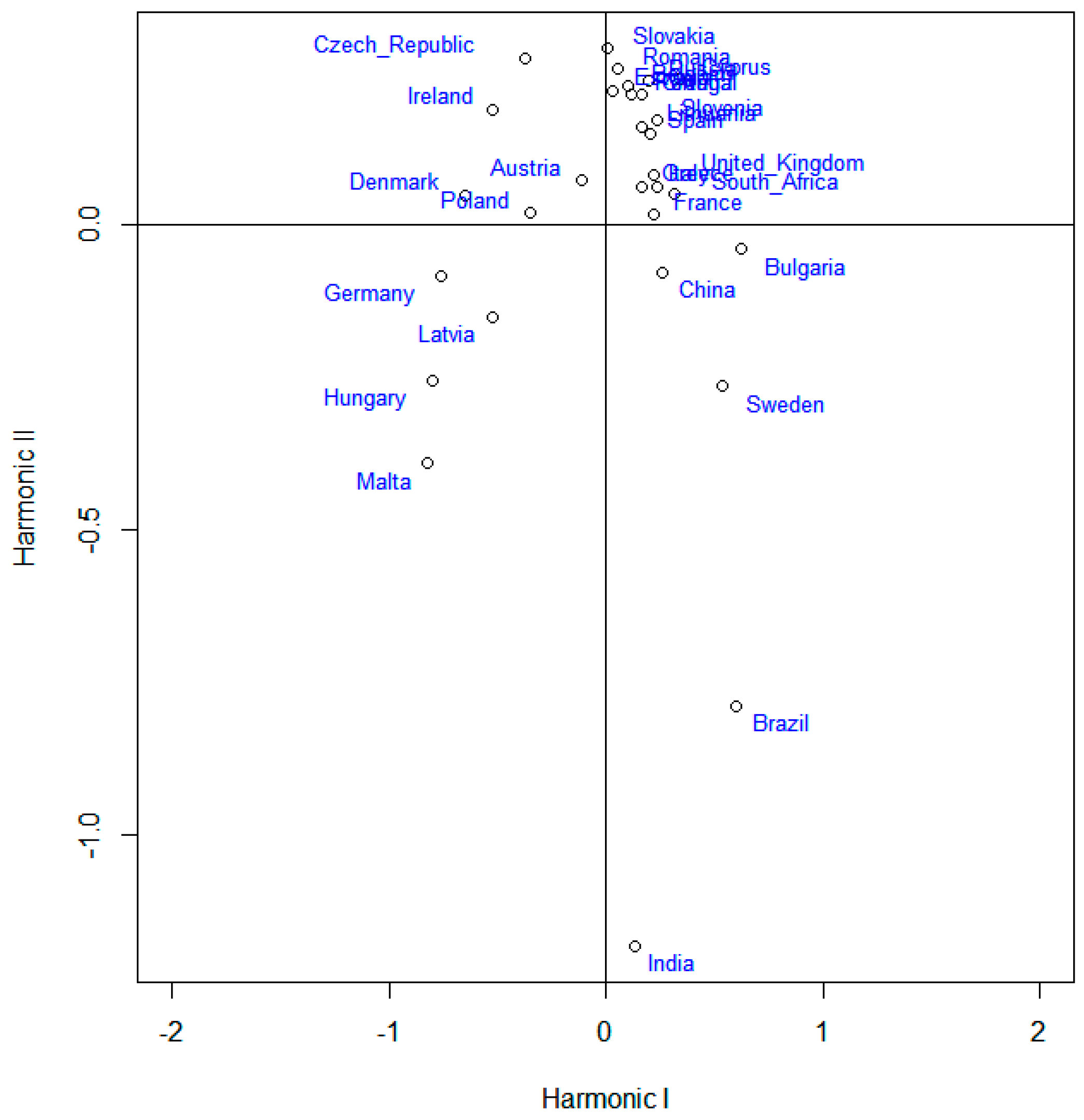
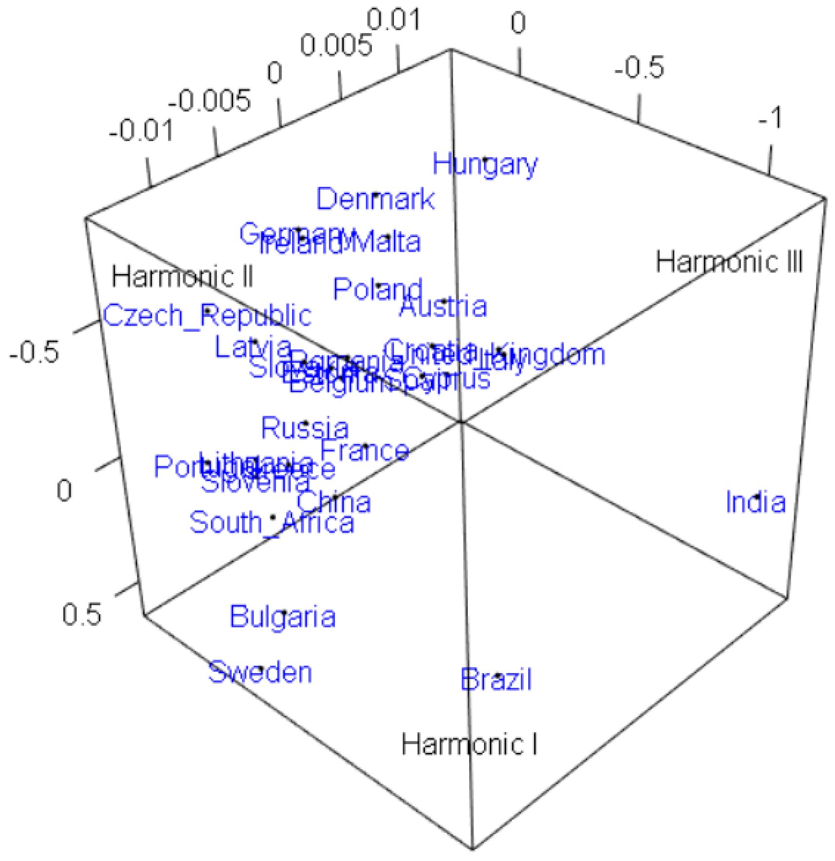
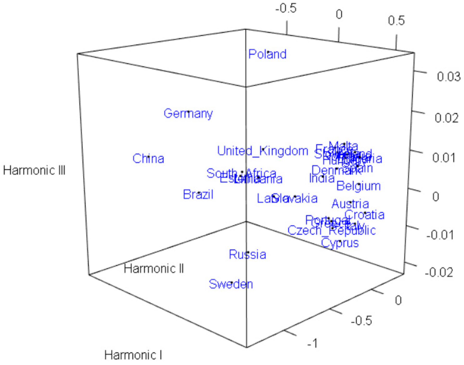
Similarly, a 2-dimensional scatter plot of the 30 countries’ government-to-GDP ratio data in the first two principal component planes constructed by using FPCA is shown in Figure 7. In addition, Figure 8 shows a 3-dimensional FPCA plot of government-to-GDP ratio with the first three principal components.

The government-to-GDP ratio classifications of Group 1, Group 2, Group 3 and Group 4 in

Table 6. Government-to-GDP ratio classification of the 30 countries.

Group	Country
Group 1	Cyprus, Croatia, Greece, Italy, Malta, Portugal, Romania, Spain, Slovenia;Belgium, France, United Kingdom, Slovakia, Estonia, Lithuania, Russia, South Africa
Group 2	Bulgaria, Sweden, China, Brazil, India
Group 3	Germany, Latvia, Hungary, Malta
Group 4	Czech Republic, Ireland, Austria, Poland, Denmark

correspond to the first, second, third and fourth quadrants in Figure 7, one by one. As can be seen from Table 6, the vast majority of EU countries that are located in Southern and Western Europe are in the first group except for Ireland and Bulgaria, and these countries had large-scale government debts after the financial crisis and the European sovereign debt crisis. The first recorded instance of a government debt default occurred in Greece, followed by Italy, Portugal, Spain and other EU countries. It should be noted that Russia and South Africa are also in the first group, which means that Russia and South Africa have similar government debt characteristics to the country of Group 1.

By analyzing Group 1, we found that the wage levels of Greece, Ireland, Portugal, Spain and Italy increased by 16.5%, 12%, 7%, 8% and 3% respectively in 2000–2008, based on the range of wage changes in Germany. If we take into account the difference of labor productivity between the above five countries and Germany, the relative increase of labor cost among the five countries in the European debt crisis from 2000 to 2008 has reached a high level of 25% to 47%. Greece and other countries with the rising labor costs, at the same time, the internal real exchange rate also rose significantly. The real exchange rates of Ireland, Greece, Spain, Italy and Portugal rose by 50%, 27%, 31%, 34% and 24% respectively, compared with Germany from 2000 to 2008. Due to the unification of monetary policy, the financing cost of peripheral countries with weak monetary strength has dropped significantly (the interest rate difference between Greek long-term bonds and German bonds has dropped from more than ten percentage points to less than 0.5 percentage points), which has significantly improved the financing capacity of peripheral countries in the euro area such as Greece. The euro system of unified monetary policy and decentralized fiscal policy encourages fiscal “free riding” of all countries, which leads to the moral hazard of large-scale and sustained fiscal deficit, and leads to the institutional continuous accumulation of government debt of Greece and other countries. Under the euro system, the unified currency fixes the exchange rate risk, the financial integration fixes the inflation risk, and the government can continue to obtain low-cost debt financing in the financial market. Therefore, governments only need to expand finance to achieve the growth goal, and the result is the excessive expansion of government debt. The government could not pay its debts once the economy of these countries was exposed to external shocks that disrupted market functioning, and this bad debt deteriorated the quality of the banks’ assets.

Germany is the main engine of euro-zone growth, and the sovereign debt crisis in Greece has gradually spread to Germany. The government-to-GDP ratio of German has risen to 79.844% in 2012. During the 2008 economic crisis, in order to get rid of the recession, Latvia received international loan assistance provided by the European Union and the International Monetary Fund (IMF) in 2009, which made Latvia face huge foreign debt pressure, and the debt level rose, accounting for 46.8% of GDP in 2010. In 2011, the government-to-GDP ratio of Hungary was 80.481% and the 10-year bond yield also exceeded 8%. In addition, influenced by the European sovereign debt crisis, Hungary’s export scale has been significantly reduced which suggests that the outlook for economic growth has worsened. Therefore, although there is no serious debt crisis in the countries of Group 3, their government-to-GDP ratio is still relatively high, threatening the economic development.

As a super sovereign currency, the issuing right of euro can only be controlled by the European Central Bank, and the central banks of member countries have no right to issue euro, so they lose the basis of regulating their currency circulation. Although Bulgaria and Sweden are European Union countries, they are not euro area countries, so they have the right to issue money, which means they have the right to make monetary policy independently, especially for expansionary monetary policy, whether through providing discount loans to commercial banks, or relaxing the monetary root through open market business, the central bank puts new flows into the market. These countries formulated and implemented prudent monetary policies to prevent the spread of sovereign debt after the Greek sovereign debt crisis. China, Brazil and India belong to Group 2, which means they are similar to Bulgaria and Sweden.

The Czech Republic, Austria and Poland are members of the Visegrad Group. They have the right to make monetary policy independently and flexible fiscal policy, which brings stable external environment to the economy. When the debt crisis happened, these countries adjusted their monetary policy in time and adopted prudent fiscal policy, which reduced the impact of the debt crisis on their economy. However, Slovakia is also a member of the Visegrad group, but gained accession to the euro-zone in 2009, which mean its loss of independent monetary rights, thus, its government-to-GDP ratio and fiscal deficit are very high, has been greatly been affected by the sovereign debt crisis.

From the results in Table 1, Table 2, Table 3 and Table 4, it can be seen that the cumulative variance contribution rate of the first three principal components gained by FPCA is higher than the contribution rate obtained from linear PCA. A comparison of Figure 1, Figure 2, Figure 3, Figure 4, Figure 5, Figure 6, Figure 7 and Figure 8 shows that the effect of the first three principal components obtained by FPCA is significantly better than the result gained by linear PCA. Especially for NPLs data, the cumulative variance contribution rate of the first three principal components obtained by FPCA reached 99.97% compared with 89.43% by linear PCA, which differs by nearly 10 percentage points. Known from the above analysis, using the FPCA method to extract the feature is much better than the linear PCA method through visualizations for the data. In addition, the extracted principal components obtained from FPCA can retain more complex information between the data.

Through visualization, we show the relationship between the NPLs ratio and government-to-GDP ratio of the 30 sample countries. Linear PCA can explain only 89.43% and 95.44% of the whole variance proportion with three PCs in the NPLs ratio and government-to-GDP ratio, respectively, but there remains room for about 11% and 5% unexplained variation. Although an outcome classification between NPLs ratio and government-to-GDP ratio was observed from the scatter plot, in some cases, the differentiation between classes was not so clear (Figure 1c and Figure 3c). Almost perfect integration was obtained when we used FPCA, as shown in Figure 5 and Figure 7. The explanatory ability of the three PCs has been greatly improved, and they account for 99.97% and 99.99% of the whole variance proportion. It is shown that FPCA explains more of the total data variance than linear PCA, the dimension reduction effect of FPCA is good and extracted principal components contain more information.

The data indicate that government debt markets of EU countries experienced a similar trend in terms of NPLs, with the size of NPLs similar across debt markets. The NPLs ratio and government-to-GDP ratio of the 25 EU countries and BRICS countries experienced a major fluctuation during 2007–2017, and was significantly affected during the 2008 global financial crisis and the 2009 European sovereign debt crisis. With the onset of the European sovereign debt crisis, we find evidence of the decoupling of debt markets. As a result, NPLs ratio and government-to-GDP ratio for the crisis countries and non-crisis countries experienced a significant upsurge. The Greek NPLs ratio increased for the countries in crisis, especially for Portugal, where the NPLs ratio almost tripled overall. However, the impact of the sovereign debt crisis is less for non-crisis countries, because the debt markets of these countries are decoupled from the Greek market. These results are consistent with the studies by Reboredo and Ugolini [3].

3.3. Biclustering Plot Results

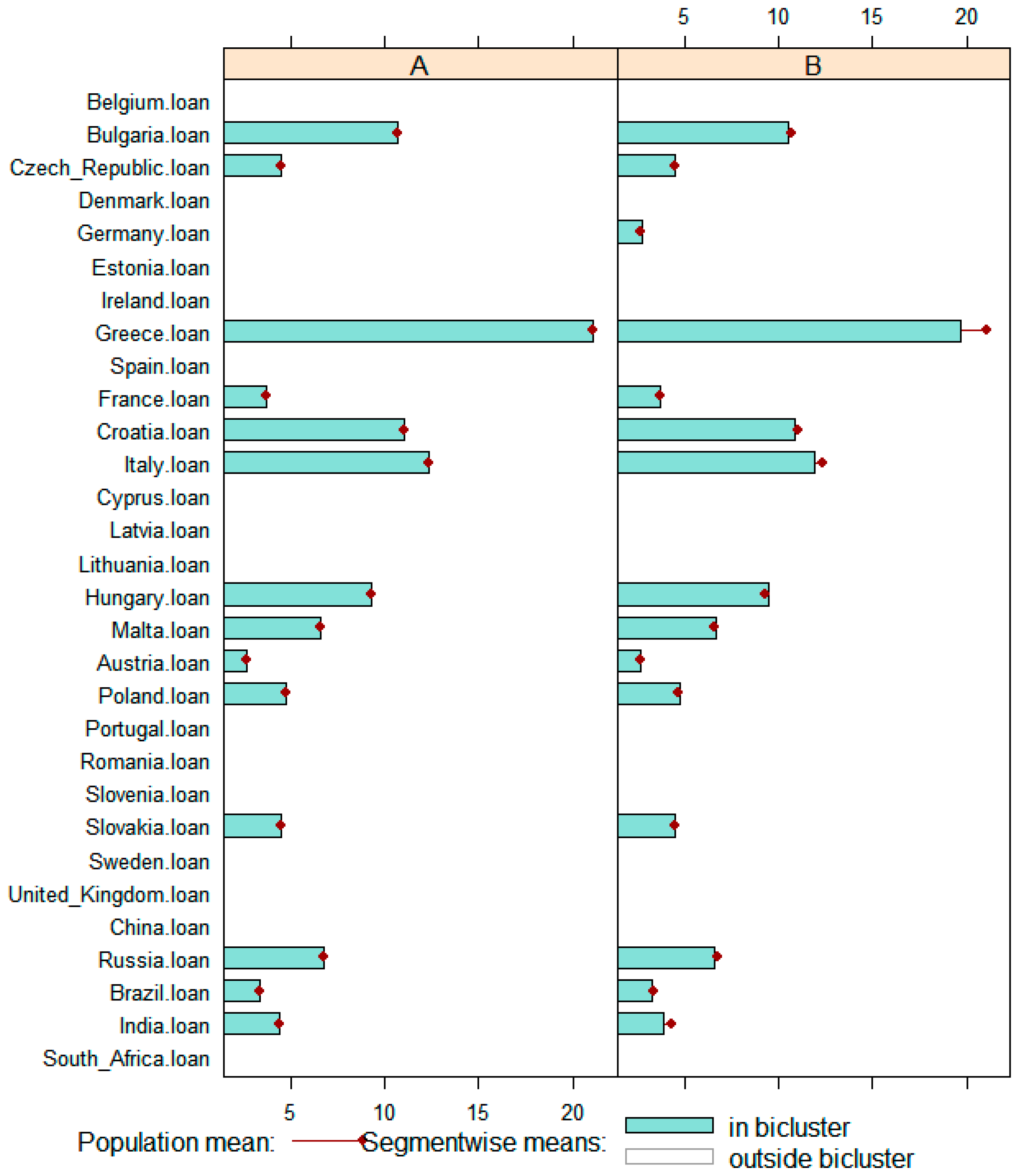
Using the proposed method, we tried to find a group of countries that showed a homogeneous pattern of NPLs and government-to-GDP ratio in a certain period. Figure 9 and Figure 10 show the biclustering plot results of NPLs and government debt, respectively. The rows and columns of the initial matrix are rearranged so that the two biclusters can be plotted together to clearly represent the relationships between them. Meanwhile, each bicluster is represented as a white or green rectangle that can be observed visually. The red lines on those areas represent the mean value for the NPLs or government-to-GDP ratio for each country.

In particular, the biclustering plot results of the 30 countries’ NPLs is drawn in Figure 9. Columns of bicluster A and bicluster B denote different groups of NPLs that different countries have in common. As shown in Figure 9, bicluster A contains 14 countries in common, including Bulgaria, Czech Republic, Greece, Italy, Hungary, Malta, Austria, Poland, Slovakia, Russia, Brazil and India. Analogously, bicluster B contains 15 countries in common, including Bulgaria, Czech Republic, Germany, Greece, Italy, Hungary, Malta, Austria, Poland, Slovakia, Russia, Brazil and India; the only difference is Germany. Thus, we conclude that the EU countries in bicluster A have experienced a wide increase of NPLs, and this crisis has also spread to Russia, Brazil and India (BRICS countries). On the other hand, bicluster B includes these countries and Germany. The reason why Germany is included in bicluster B is that the NPLs in Germany are lower than in the 14 countries.

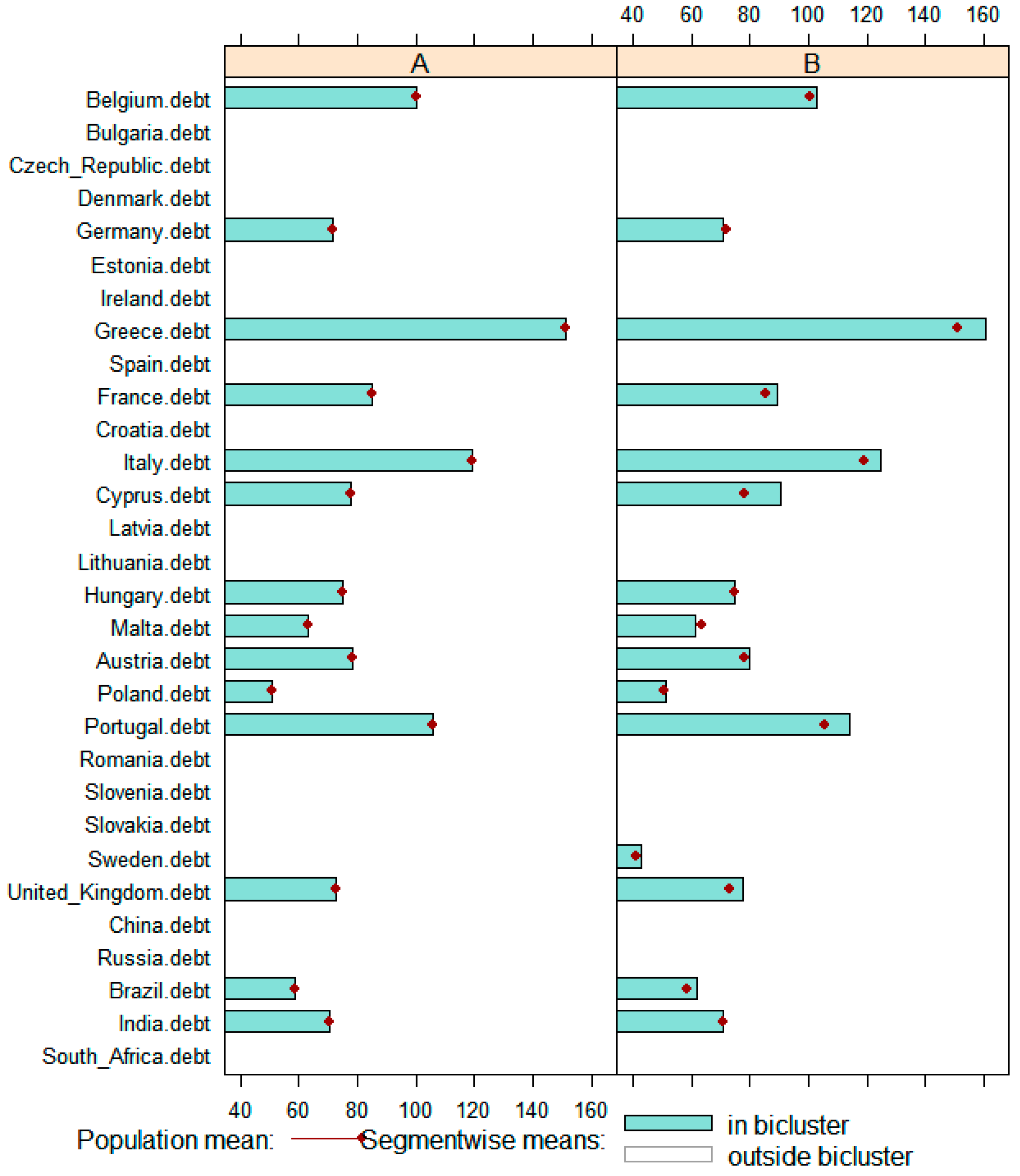
The biclustering plot results of the 30 countries’ government debt is shown in Figure 10. As can be seen, columns of bicluster A and bicluster B denote different groups of government-to-GDP ratios that different countries have in common. Bicluster A contains 14 countries in common, including Belgium, Germany, Greece, France, Italy, Cyprus, Hungary, Malta, Austria, Poland, Portugal, United Kingdom, Brazil and India. Analogously, bicluster B contains 15 countries in common, including Belgium, Germany, Greece, France, Italy, Cyprus, Hungary, Malta, Austria, Poland, Portugal, Sweden, United Kingdom, Brazil and India; the only difference is Sweden. Therefore, the biclustering visualization results show that the EU countries in bicluster A have large-scale government debts, and this phenomenon has also spread to Brazil and India. In addition, bicluster B includes these countries as well as Sweden, because the government-to-GDP ratio of Sweden is lower than in the 14 countries.

There are many economic links between BRICS countries, just as there are similar links between EU countries. However, EU countries have much closer fiscal linkages regarding sovereign debt than BRICS countries. Before the breakout of the financial crisis and debt crisis, the NPLs ratios of EU countries in government debt markets were similar. However, government debt markets decoupled with the breakout of the debt crisis, and crisis countries are even more contagious, mainly for the countries in crisis and particularly negatively for the countries of bicluster A. As a result, the NPLs ratio increased for the government debt markets for the non-crisis countries. If a financial or sovereign debt crisis is driven by the common shocks of macroeconomic fundamentals, the level of crisis in the EU countries will be higher than that in the BRICS countries. Thus, the outbreak of the European sovereign debt crisis was because of the common vulnerability of the EU countries to major adverse events, as proposed by Ang and Longstaff [42].

3.4. Discussion

This article visualizes bank non-performing loans (NPLs) and government debt distress data integration and an outcome classification after the outbreak of European sovereign debt. To extract the main feature of the sample data, dimensionality reduction was done by linear PCA. The results obtained from linear PCA suggest that the variance contribution rate of the first three principal components accounts for more than 89% of the cumulative proportion. Moreover, we have shown that some countries are clustered together by using 2-D and 3-D visualizations.

We employed FPCA to extract more complex clustering features. The results indicate that the first three principal components obtained from FPCA explain a higher percent of the cumulative variance contribution rate as compared to the linear principal components. It is shown that FPCA explains more of the total data variance than linear PCA, the dimension reduction effect of FPCA is good, and extracted principal components contain more information. This finding is in line with the existing results of Jiang and Yan [22]. In addition, the figures of 2D and 3D visualizations have shown the clustering pattern of NPLs and government debt data.

A biclustering method was used to discover biclusters in the sample data. Our experimental results show that the pattern of biclusters represents significant meaning. It can be seen that columns of bicluster A and bicluster B denote different groups of NPLs (or government debt) that different countries have in common.

The implication of these results is that the government debt, as well as NPLs of EU and BRICS countries, increased drastically after the global financial crisis and the European debt crisis. Specifically, most Southern and Western European countries are under the greatest pressure whether on NPLs or government debt, followed by Eastern European, Central European and Northern European countries. It should be noted that there is a sharp increase in NPLs and government debt for BRICS countries after a crisis, which means that those crises spread to emerging countries. Our findings provide support to several recent studies that government debt incentives to default increase if a government cannot pay its debts, and their effects on the economy would be amplified through the impact on banks’ balance sheets [43].

4. Conclusions

In this study, we examined the visualization of NPLs and government-to-GDP ratio integration and an outcome classification in Eurozone and BRICS countries after the global financial crisis of 2008 and the subsequent European debt crisis of 2009. In particular, our sample countries contain developed countries and developing countries, and they also include countries with debt crises and no debt crises over the same time period. We first provide evidence, by using PCA and FPCA, that the variance contribution rate of the first three principal components obtained by FPCA is significantly higher than PCA. It can be found that the first three principal components obtained by FPCA have a good dimensionality reduction effect, and the obtained first three principal components contain more data information. We also found that the government debt and NPLs of EU and BRICS countries increased drastically after a crisis, and crisis countries are contagious. However, the impact of the Greek debt crisis was lower for non-crisis countries, because the debt markets of these countries are decoupled from the Greek market. Furthermore, evidence also confirms that sovereign debtors in the EU countries have much closer fiscal linkages than BRICS countries. The level of crisis in the EU countries will be higher than that in the BRICS countries if crisis is driven by the common shocks of macroeconomic fundamentals.

Our findings in this article confirm that countries with high government debt have experienced a significant increase in their contribution to systemic risk since 2008, especially for EU countries. The results may have some meaningful implications for policymakers because unsustainable government debt can lead to payment defaults, which will impose more problems on the stability of the region. Furthermore, the findings in this paper can also help to establish a better monitoring mechanism and, ultimately, impose penalties on countries that violate regulations.

References

1. Alessandri, P.; Haldane, A.G. Banking on the State; Bank of England: London, UK, 2009; Volume 15, p. 448. [Google Scholar]
2. Eichengreen, B.; Wyplosz, C. How the euro crisis was successfully resolved. J. Econ. 2016, 98, 463–484. [Google Scholar]
3. Reboredo, J.C.; Ugolini, A. Systemic risk in European sovereign debt markets: A CoVaR-copula approach. J. Int. Money Financ. 2015, 51, 214–244. [Google Scholar] [CrossRef]
4. Gertler, M.; Kiyotaki, N.; Queralto, A. Financial crises, bank risk exposure and government financial policy. J. Monet. Econ. 2012, 59, S17–S34. [Google Scholar] [CrossRef]
5. Pagano, M.S.; Sedunov, J. A comprehensive approach to measuring the relation between systemic risk exposure and sovereign debt. J. Financ. Stab. 2016, 23, 62–78. [Google Scholar] [CrossRef]
6. Papadamou, S.; Kyriazis, N.A.; Tzeremes, P.G. Spillover effects of US QE and QE tapering on African and Middle Eastern etock indices. J. Risk Financ. Manag. 2019, 12, 57. [Google Scholar] [CrossRef] [Green Version]
7. Papadamou, S.; Kyriazis, N.A.; Tzeremes, P.G. Unconventional monetary policy effects on output and inflation: A metaanalysis. Int. Rev. Financ. Anal. 2019, 61, 295–305. [Google Scholar] [CrossRef]
8. Morais, B.; Peydró, J.L.; Roldán-Peña, J.; Ruiz-Ortega, C. The international bank lending channel of monetary policy rates and QE: Credit supply, reach-for-yield, and real effects. J. Financ. 2019, 74, 55–90. [Google Scholar] [CrossRef] [Green Version]
9. Reinhart, C.M.; Rogoff, K.S. The aftermath of financial crises. Am. Econ. Rev. 2009, 99, 466–472. [Google Scholar] [CrossRef] [Green Version]
10. Reinhart, C.M.; Rogoff, K.S. Growth in a time of debt (nber working paper version). Am. Econ. Rev. 2010, 100, 573–578. [Google Scholar] [CrossRef] [Green Version]
11. Louzis, D.P.; Vouldis, A.T.; Metaxas, V.L. Macroeconomic and bank-specific determinants of non-performing loans in Greece: A comparative study of mortgage, business and consumer loan portfolios. Work. Pap. 2012, 36, 1012–1027. [Google Scholar] [CrossRef]
12. Reboredo, J.C.; Ugolini, A. A vine-copula conditional value-at-risk approach to systemic sovereign debt risk for the financial sector. N. Am. J. Econ. Financ. 2015, 32, 98–123. [Google Scholar] [CrossRef]
13. Makri, V.; Tsagkanos, A.; Bellas, A. Determinants of non-performing loans: The case of Eurozone. Panoeconomicus 2014, 61, 193–206. [Google Scholar] [CrossRef] [Green Version]
14. Ghosh, A. Banking-industry specific and regional economic determinants of non-performing loans: Evidence from US states. J. Financ. Stab. 2015, 20, 93–104. [Google Scholar] [CrossRef]
15. Jiang, Q.C.; Yan, X. Monitoring multi-mode plant-wide processes by using mutual information-based multi-block PCA, joint probability, and Bayesian inference. Chemom. Intell. Lab. Syst. 2014, 136, 121–137. [Google Scholar] [CrossRef]
16. Bakdi, A.; Kouadri, A.; Bensmail, A. Fault detection and diagnosis in a cement rotary kiln using PCA with EWMA-based adaptive threshold monitoring scheme. Control Eng. Pract. 2017, 66, 64–75. [Google Scholar] [CrossRef]
17. Yu, H.; Chen, R.; Zhang, G. A SVM stock selection model within PCA. Procedia Comput. Sci. 2014, 31, 406–412. [Google Scholar] [CrossRef] [Green Version]
18. Mazumder, R.; Hastie, T.; Tibshirani, R. Spectral regularization algorithms for learning large incomplete matrices. J. Mach. Learn. Res. 2010, 99, 2287–2322. [Google Scholar]
19. Candès, E.J.; Sing-Long, C.A.; Trzasko, J.D. Unbiased risk estimates for singular value thresholding and spectral estimators. Trans. Signal Process. 2013, 61, 4643–4657. [Google Scholar] [CrossRef] [Green Version]
20. Florackis, C.; Palotás, K. Corporate governance and performance: New evidence using nonlinear principal component analysis. Adv. Quant. Anal. Financ. Account. 2012, 10, 38. [Google Scholar]
21. Stoica, O.; Mehdian, S.; Sargu, A. The impact of internet banking on the performance of Romanian banks: DEA and PCA approach. Procedia Econ. Financ. 2015, 20, 610–622. [Google Scholar] [CrossRef] [Green Version]
22. Jiang, Q.C.; Yan, X.F. Parallel PCA-KPCA for nonlinear process monitoring. Control Eng. Pract. 2018, 80, 17–25. [Google Scholar] [CrossRef]
23. Kim, J.M.; Jung, H.; Economics, A.; Phillips, A. Relationship between oil price and exchange rate by FDA and copula. Appl. Econ. 2017, 50, 2486–2499. [Google Scholar] [CrossRef]
24. Jaimungal, S.; Ng, E.K.H. Consistent functional PCA for financial time-series. In Proceedings of the Iasted International Conference on Financial Engineering & Applications, Berkeley, CA, USA, 24–26 September 2007; pp. 103–108. [Google Scholar]
25. Densing, M. Occupation times of the Ornstein-Uhlenbeck process: Functional PCA and evidence from electricity prices. Phys. A Stat. Mech. Appl. 2012, 391, 5818–5826. [Google Scholar] [CrossRef]
26. Guharay, S.K.; Thakur, G.S.; Goodman, F.J.; Rosen, S.L.; Houser, D. Integrated data-driven analytics to identify instability signatures in nonstationary financial time series. Appl. Econ. 2016, 48, 1678–1694. [Google Scholar] [CrossRef]
27. Morseletto, P. Analyzing the influence of visualizations in global environmental governance. Environ. Sci. Policy 2017, 78, 40–48. [Google Scholar] [CrossRef]
28. Zhang, Y.; Zha, H.; Chu, C.H. A Time-Series Biclustering Algorithm for Revealing Co-Regulated Genes. In Proceedings of the International Conference on Information Technology: Coding and Computing (ITCC’05), Las Vegas, NV, USA, 4–6 April 2005. [Google Scholar]
29. Lee, J.H.; Lee, Y.R.; Jun, C.H.A. Biclustering method for time series analysis. Ind. Eng. Manag. Syst. 2010, 9, 131–140. [Google Scholar] [CrossRef]
30. Huang, Q.H. Discovery of time-inconsecutive co-movement patterns of foreign currencies using an evolutionary biclustering method. Appl. Math. Comput. 2011, 218, 4353–4364. [Google Scholar] [CrossRef]
31. Xue, Y.; Liu, Z.; Luo, J.; Ma, Z.; Zhang, M.; Hu, X.; Kuang, Q. Stock market trading rules discovery based on biclustering method. Math. Probl. Eng. 2015. [Google Scholar] [CrossRef]
32. Pearson, K. On lines and planes of closest fit to system of points in space. Philos. Mag. Ser. 1901, 6, 559–572. [Google Scholar] [CrossRef] [Green Version]
33. Lu, B.W.; Pandolfo, L. Quasi-objective nonlinear principal component analysis. Neural Netw. 2011, 24, 159–170. [Google Scholar] [CrossRef] [PubMed]
34. Kazor, K.; Holloway, R.W.; Cath, T.Y.; Hering, A.S. Comparison of linear and nonlinear dimension reduction techniques for automated process monitoring of a decentralized wastewater treatment facility. Stoch. Environ. Res. Risk Assess. 2016, 30, 1527–1544. [Google Scholar] [CrossRef]
35. Santos, A.D.F.; Silva, M.F.M.; Sales, C.S.; Costa, J.C.W.A.; Figureueiredo, E. Applicability of linear and nonlinear principal component analysis for damage detection. In Proceedings of the IEEE International Instrumentation and Measurement Technology Conference (I2MTC) Proceedings, Pisa, Italy, 11–14 May 2015. [Google Scholar]
36. Shao, R.; Hu, W.; Wang, Y.; Qi, X. The fault feature extraction and classification of gear using principal component analysis and kernel principal component analysis based on the wavelet packet transform. Measurement 2014, 54, 118–132. [Google Scholar] [CrossRef]
37. Cheng, Y.; Church, G.M. Biclustering of expression data. In Proceedings of the 8th International Conference on Intelligent Systems for Molecular Biology, San Diego, CA, USA, 19–23 August 2000; Volume 8, pp. 93–103. [Google Scholar]
38. Kim, J.M.; Kim, N.K.; Jung, Y.S.; Jun, S.H. Patent data analysis using functional count data model. Soft Comput. 2018, 23, 8815–8826. [Google Scholar] [CrossRef]
39. Ramsay, J.O.; Silverman, B.W. Functional data analysis. Int. Encycl. Soc. Behav. Sci. 2001, 40, 5822–5828. [Google Scholar]
40. Craven, P.; Wahba, G. Smoothing noisy sata with spline functions: Estimating the correct degree of smoothing by the method of generalized cross validation. Numer. Math. 1979, 31, 377–403. [Google Scholar] [CrossRef]
41. Yoon, J.E.; Kim, J.M.; Hwang, S.Y. Functional ARCH (fARCH) for high-frequency time series: Illustration. Korean J. Appl. Stat. 2017, 30, 983–991. [Google Scholar]
42. Ang, A.; Longstaff, F.A. Systemic sovereign credit risk: Lessons from the U.S. and Europe. J. Monet. Econ. 2013, 60, 493–510. [Google Scholar] [CrossRef]
43. Gennaioli, N.; Martin, A.; Rossi, S. Sovereign default, domestic banks and financial institutions. J. Financ. 2014, 69, 819–866. [Google Scholar] [CrossRef]
Figure 1. Scatter plots of the 30 countries’ NPLs data in the principal component (PC1, PC2 and PC3) plane obtained by using linear PCA. Panel (a) displays the PC1–PC2 plane, (b) the PC1–PC3 plane, and (c) the PC2–PC3 plane.
Sustainability 12 00131 g001aSustainability 12 00131 g001b
Figure 2. The 3-dimensional space of 30 countries’ NPLs data obtained by using linear PCA.
Sustainability 12 00131 g002
Figure 3. Scatter plots of the 30 countries’ government-to-GDP ratio data in the principal component (PC1, PC2, and PC3) plane obtained by using linear PCA. Panel (a) displays the PC1–PC2 plane, (b) the PC1–PC3 plane, and (c) the PC2–PC3 plane.
Sustainability 12 00131 g003
Figure 4. The 3-dimensional space of 30 countries’ government-to-GDP ratio data obtained by using linear PCA.
Sustainability 12 00131 g004
Figure 5. 2D plot of the 30 countries’ bank NPLs data in the principal component plane obtained by using FPCA.
Sustainability 12 00131 g005
Figure 6. 3D space of 30 countries’ NPLs data obtained by using FPCA.
Sustainability 12 00131 g006
Figure 7. 2D plot of the 30 countries’ government-to-GDP ratio data in the principal component plane obtained by using FPCA.
Sustainability 12 00131 g007
Figure 8. 3D space of 30 countries’ government-to-GDP ratio obtained by using FPCA.
Sustainability 12 00131 g008
Figure 9. Biclustering plot of the 30 countries’ NPLs.
Sustainability 12 00131 g009
Figure 10. Biclustering plot of 30 countries’ government-to-GDP ratio.
Sustainability 12 00131 g010