Monitoring Phenology in the Temperate Grasslands of China from 1982 to 2015 and Its Relation to Net Primary Productivity

Abstract

Both vegetation phenology and net primary productivity (NPP) are crucial topics under the background of global change, but the relationships between them are far from clear. In this study, we quantified the spatial-temporal vegetation start (SOS), end (EOS), and length (LOS) of the growing season and NPP for the temperate grasslands of China based on a 34-year time-series (1982–2015) normalized difference vegetation index (NDVI) derived from global inventory modeling and mapping studies (GIMMS) and meteorological data. Then, we demonstrated the relationships between NPP and phenology dynamics. The results showed that more than half of the grasslands experienced significant changes in their phenology and NPP. The rates of their changes exhibited spatial heterogeneity, but their phenological changes could be roughly divided into three different clustered trend regions, while NPP presented a polarized pattern that increased in the south and decreased in the north. Different trend zones’ analyses revealed that phenology trends accelerated after 1997, which was a turning point. Prolonged LOS did not necessarily increase the current year’s NPP. SOS correlated with the NPP most closely during the same year compared to EOS and LOS. Delayed SOS contributed to increasing the summer NPP, and vice versa. Thus, SOS could be a predictor for current year grass growth. In view of this result, we suggest that future studies should further explore the mechanisms of SOS and plant growth.

1. Introduction

Vegetation phenology is a sensitive and critical renewal indicator that presents vegetation change in response to climate change because vegetation phenology plays an important role in many biological processes, such as the carbon balance of the ecosystem [1]. The SOS and EOS (start and end of the growing season dates) are the most frequently measured phenology indicators, so the growing season length is defined as the difference of the SOS and EOS. Under the background of dramatic global climate change [2], rapid shifts in plant phenology will influence terrestrial ecosystems’ structures and functions, as these shifts affect vegetation surface albedo, heat flux, and even water and carbon exchange [3,4,5]. Numerous studies have documented plants’ phenological responses to recent climate change across a wide range of different zones, but no comprehensive conclusion has been reached because the mechanisms that drive long-term changes in phenology are still unclear [6,7]. The ecosystem’s carbon cycle is vital to humans from a natural environmental and economic perspective [8]. The net primary productivity (NPP), as the amount of carbon intake from the atmosphere by plants after assimilation through photosynthesis minus autotrophic respiration [9], represents the natural vegetation of carbon fixation and is also used to monitor the biomass yields of pastures, crops, and forests because it is relatively easy to measure [9,10,11,12,13,14].

Both the primary production and vegetation phenology are strongly dependent on climate conditions and physiographic characteristics. Monitoring the spatiotemporal dynamics of productivity and phenology could improve our understanding of climate change and ecosystem variability. Climatic limitations on plant production can include temperature, moisture availability, and incident photosynthetic active radiation. The geographic distribution of climate limitations for plant growth is not uniform, and multiple factors are often colimiting to growth [15]. It is intuitively assumed that warming will prolong the length of the growing season, and increased productivity is expected to result immediately from the fact that more active growing days are available for photosynthesis. Indeed, past studies have demonstrated that a prolonged growing season is coupled with increased annual productivity [16,17,18]. On the contrary, warming climate-induced water stress restrains plant photosynthesis in the summer and reduces peak summer productivity (or even the whole year’s productivity). Recent studies have also reported that a shortened and length of the growing season (LOS) (a delayed SOS and/or an advanced EOS) is beneficial for increasing productivity [19,20]. The relationship between phenology and productivity shows significant variation in different regions and among different vegetation types. These contradictory results suggest that the mechanisms of interaction between phenology and productivity are complicated and still unclear. In addition, grasslands are one of the most widely distributed vegetation types on earth [21]. Grasslands also account for more than 40% of the terrestrial area of China and are an important component of the terrestrial ecosystem, which is sensitive to climate change [22]. In particular, the temperate grasslands of China are a crucial ecological barrier, featuring high quality natural pastures and facilitating important livestock husbandry. Understanding the relationship between phenology and grassland productivity provides a scientific basis for the rational management of the grazing season.

The primary purpose of this study was to characterize the spatial long-term variation in phenology (i.e., SOS, EOS, and LOS) and NPP over the period 1982–2015 in the temperate grasslands of China, based on using the normalized difference vegetation index (NDVI) derived from global inventory modeling and mapping studies (GIMMS). Then, we detected the changes in the trends of both productivity and phenology over the past decades. Lastly, we dominantly quantified the relationship between NPP and phenology on a pixel scale and explored the possible environmental control mechanisms of interannual variations. These results will improve our understanding of the potential variabilities of phenology and grass growth under climate change in this region.

2. Materials and Methods

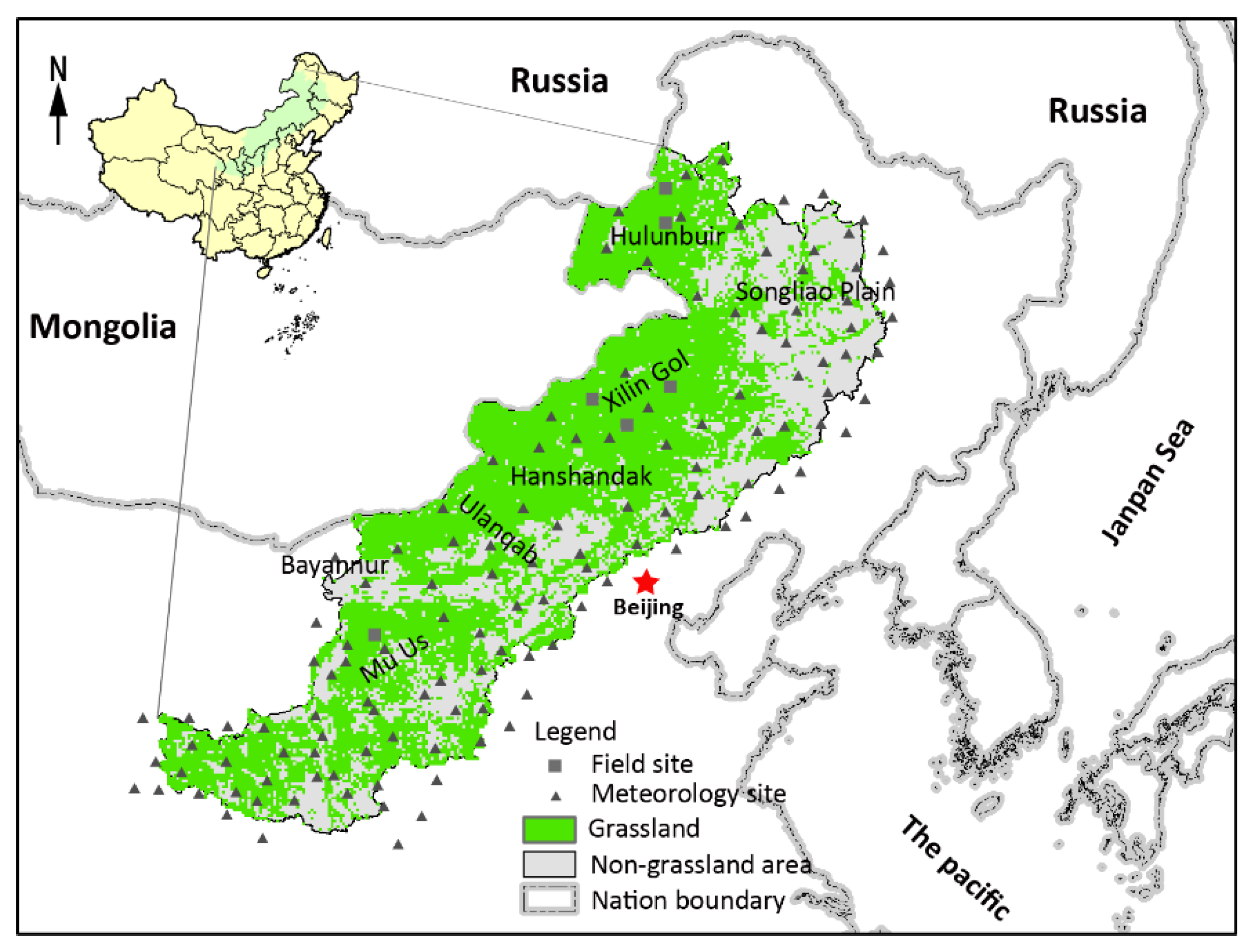
2.1. Study Area

The temperate grasslands of China are mainly distributed across the Songliao plain, the Inner Mongolian Plateau, and the Loess Plateau from east to west, and end at the east edge of the Qin–Tibet Plateau [23] (Figure 1). This region is of a temperate continental monsoon climate, featuring four distinct seasons annually, with rain and heat during the same period, precipitation less than 500 mm, and annual average temperatures varying from −5 to 10 °C. The elevation of this zone is higher from east to west, with a range approximately from 90 to 4300 m.

2.2. Data Source and Processing

2.2.1. NDVI Datasets

The GIMMS NDVI-3g is the latest version, termed the third-generation NDVI dataset, acquired by the NOAA (National Oceanic and Atmospheric Administration) satellite and produced by the global inventory modeling and mapping studies. This dataset was assembled from several AVHRR (Advanced Very-High-Resolution Radiometer) and SeaWiFS (Sea-Viewing Wide Field-of-View Sensor) sensors, and the algorithm improved the quality of the results by accounting for deleterious effects, such as calibration loss, orbital drift, volcanic eruption, solar zenith angle, etc. [24]. This version’s dataset has a 0.05 degree (about 8 km) spatial resolution and a semimonthly maximum value composite (MVC) in a time series.

2.2.2. Meteorological Data

Three types of monthly meteorological data (precipitation, temperature, and radiation) were downloaded from the National Meteorological Information Center (http://data.cma.cn/data). The grid meteorological data matching the NDVI resolution were interpolated using the Partial Thin Plate Smoothing Splines method based on topography via the ANUSPLIN software (version 4.3) [25].

2.2.3. Land Cover

The grassland was distributed according to the land-use dataset, WESTDC (version 2.0), prepared by the Cold and Arid Regions Environmental and Engineering Research Institute of China, National Natural Science Foundation of China (http://westdc.westgis.ac.cn). This land-use dataset was produced by the Chinese Academy of Sciences from aerial photographs and Landsat TM (Thematic Mapper) and ETM (Enhanced TM) images, combining 1:100,000 land-use map field surveys.

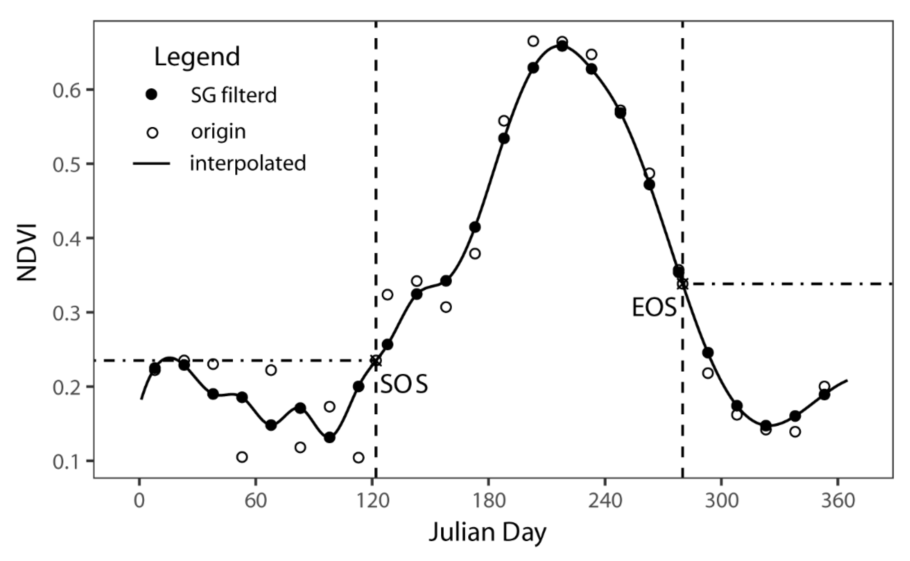
2.3. Phenological Metrics Extraction

Although the GIMMS NDVI has been corrected several times [24], there remains perceptible residual noise in the time-series NDVI due to the atmosphere (cloud, dust, etc.), sensors, and surface bidirectional reflectance, which affects dataset continuity, necessitating an effective algorithm to reduce the influence of noise to improve the quality of the time-series values. Plenty of noise-reduction methods (smoothing methods) for reconstructing time-series have been proposed and are frequently used, such as the best index of slope extraction [26], Savitzky–Golay filtering (SG) [27], Asymmetric Gaussian fitting [28], etc., but there is still no conclusive evidence that any one method is stronger than the others. In this study, SG was chosen to reduce drop-outs, gaps, and needlepoint humps from the NDVI time-series curve. After smoothing, we reconstructed the semimonth time-series NDVI dataset (Figure 2). To detect the phenology of each year for each date, the daily NDVI must be obtained. We interpolated the semi-month NDVI with Julian days using a six degree polynomial function [6].

The dynamic threshold method [29] was selected to detect phenology with the reconstructed NDVI series. Each pixel time-series NDVI in one year was assessed with a transformation, as per Equation (1):

$$NDV{I}_{ratio} = \frac{NDVI-NDV{I}_{min}}{NDV{I}_{max}-NDV{I}_{min}}$$

(1)

where NDVI is the daily NDVI values from interpolation, $NDV{I}_{max}$ is defined as the average of the ten maximum daily NDVIs, and $NDV{I}_{min}$ is the average of the ten minimum daily NDVIs. The purpose of using the average is to weaken the influence of extreme values. The $NDV{I}_{ratio}$ is the output ratio. Then, we used an $NDV{I}_{ratio}$ equal to 25% as the threshold to extract the SOS and a ratio equal to 30% for the EOS [30,31]. Hence, LOS was calculated as the difference between the SOS and EOS.

2.4. NPP Estimation

Field measurements of NPP are only practical for small areas and always lack long-term continuous records. For larger regional scale areas and temporal continuous series data, model calculation is considered to be an effective alternative for estimating the historical NPP. Though a variety of models have been created for NPP estimation and other components of the carbon cycle, the CASA (Canegie–Ames–Stanford Approach) model is an excellent light-use efficiency model, which has been applied and verified in many different areas [32,33,34,35].

The basic principle of the CASA model equation is applied to the spatial region as follows:

$$NPP\left(x,t\right)=APAR\left(x,t\right)\times ϵ\left(x,t\right)$$

(2)

where x is the spatial location (pixels) and t is a certain time node. APAR is obtained by

$$APAR\left(x,t\right)=FPAR\left(x,t\right)\times SOL\left(x,t\right)\times 0.5$$

(3)

where FPAR is the fraction of the photosynthetic active radiations absorbed by the vegetation canopy; SOL is the total solar radiation (MJ/m²); and the constant 0.5 stands for the fraction of solar radiation that can be used by the vegetation.

$$ϵ\left(x,t\right)=T_{ϵ1}\left(x,t\right)\times T_{ϵ2}\left(x,t\right)\times W_{ϵ}\left(x,t\right)\times {ϵ}_{max}$$

(4)

where $T_{ϵ1}$ and $T_{ϵ2}$ are the temperature stress effects on the light use efficiency of vegetation. $W_{ϵ}$ is the moisture stress effect. ${ϵ}_{max}$ is the maximum light use efficiency under optimum conditions, which is set as 0.389 gC/MJ in this study area. More details on the CASA model can be found in references [35,36,37].

2.5. Analysis and Statistics

The Theil–Sen median slope estimate [38,39] was applied to temporal linear trend regression, as this estimate is more robust, effective, and unaffected by the outlier trend detection method than least squares regression. This method chooses the median slope among all lines through paired sample points for a general linear regression model, as follows:

$$y=\alpha +\beta x+ϵ$$

(5)

where x and y are variables; $\alpha$ is interception; $\beta$ is the slope of a monotonous straight line; and ϵ is the residual of fit. For a time series $Y=\left\{y_p,y_{p+1},\dots ,y_{p+n}\right\}$, the independent value is the continuous year ordinal. The Theil–Sen slope $\beta$ is calculated as follows:

$$\beta =Median\left(\frac{y_j-y_i}{i-j}\right),p\le j<i\le p+n.$$

(6)

The piecewise regression model [40] was adopted to detect the turning points of the time series variation.

$$y=\{\begin{array}{c}\alpha +{\beta }_{1}x+ϵ, x<x_p\\ \alpha +{\beta }_{1}x+{\beta }_2\left(x-x_p\right)+ϵ, x\ge x_p\end{array}.$$

(7)

what separates piecewise regression from general linear regression is that piecewise regression contains extra $x_p$ as turning points. In order to determine reasonable turning points, we constrained $x_p$ within an artificial range.

The Pearson correlation coefficient was used to measure the relationship of two variables in each pixel [41]. Before calculating the coefficient, Min–Max Normalization was applied to each variable. All data processing was performed in the R software (version 3.4).

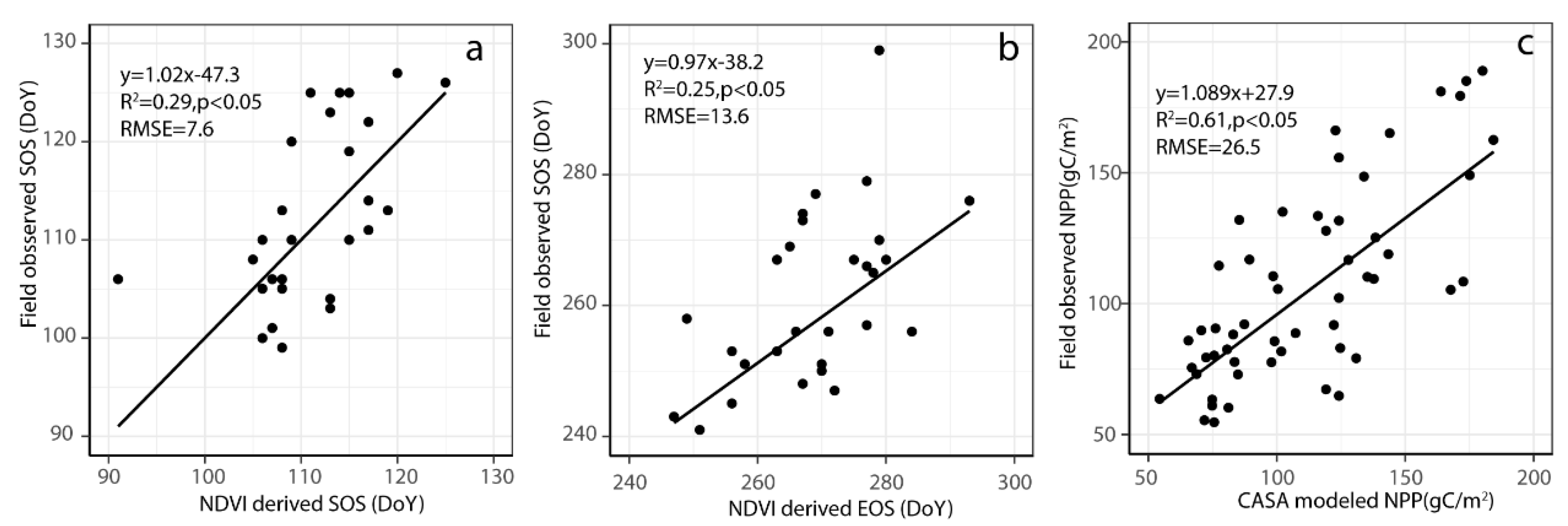
2.6. Model Validation

The grassland green-up and withering periods were acquired from the Inner Mongolia Meteorology Station, and the grassland biomass data were measured from 63 quadrate plots in August 2009. Figure 3a,b shows the correlation between the field-observed and NDVI-derived phenology (SOS and EOS). Both were marginally significant, with an R² of 0.29 and 0.25 (p < 0.05) and a root mean square error (RMSE) of 7.6 and 13.6 d, respectively. These relationships are similar to those of a previous study on temperate vegetation in China [20]. Figure 3c presents the result of the correlation analysis between the field-observed NPP and the CASA-modeled NPP. The correlation was significant (R² = 0.61, p < 0.01, n = 63), which suggests that the accuracy of the model’s results was sufficient, and that the CASA model can be used to estimate the changes in actual NPP for the temperate grassland of China.

3. Result

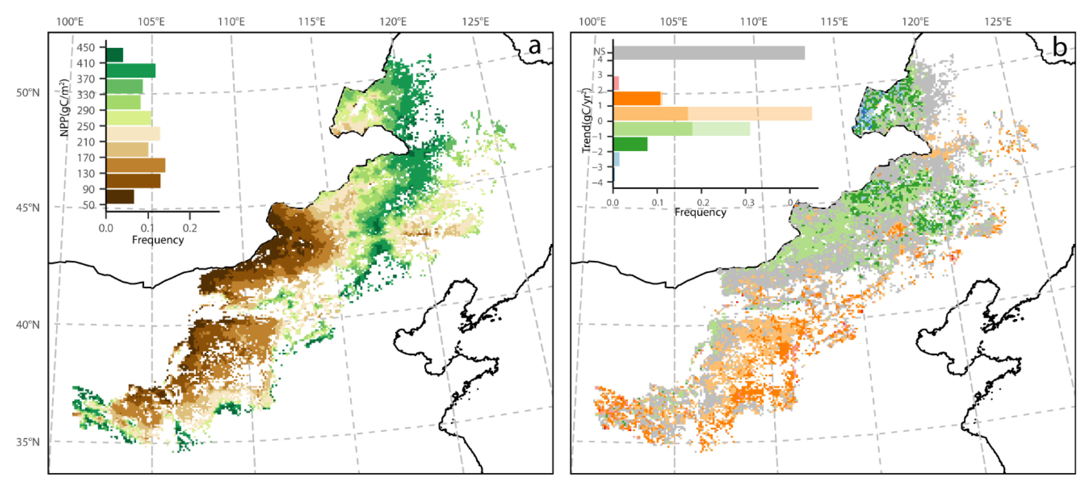
3.1. Mean Spatial Patterns of Phenology and NPP

The spatial patterns of the average phenology metrics (SOS, EOS, and LOS) over the past 32 years (1982–2013) are depicted in Figure 4. The SOS ranged chiefly from approximately 100 d (Julian days, the same below) to 120 d, which accounted for 98.7% of the total grassland area. Only 1.3% of the areas began the growing season outside of this range. Furthermore, the SOS were divided into two main groups. Early SOS (before 110 d) was found in the typical grasslands of Inner Mongolia (e.g., the west of Hulubiur, Xilin Gol, and the north of Ulanqab), while the later SOS (after 110 d) was mainly found in the rest of the study area (e.g., the Songneng Plain of China and the Loess Plateau) (Figure 4a). The EOS had a very dominant range of 258–276 d, which accounted for 97.3% of the total grassland area. In contrast with the SOS spatial distribution, the EOS of the typical grassland in Inner Mongolia and the Loess Plateau appeared later than the EOS of other areas (Figure 4c). The LOS spatial pattern was generally similar to that of EOS (Figure 4e). The long-term mean NPP ranged from 27.2 to 463.6 gC/m², with a decreasing trend from southeast to northeast, which was dependent on precipitation distribution due to decreases in monsoon moisture from the near coastal area to the inland (Figure 5a).

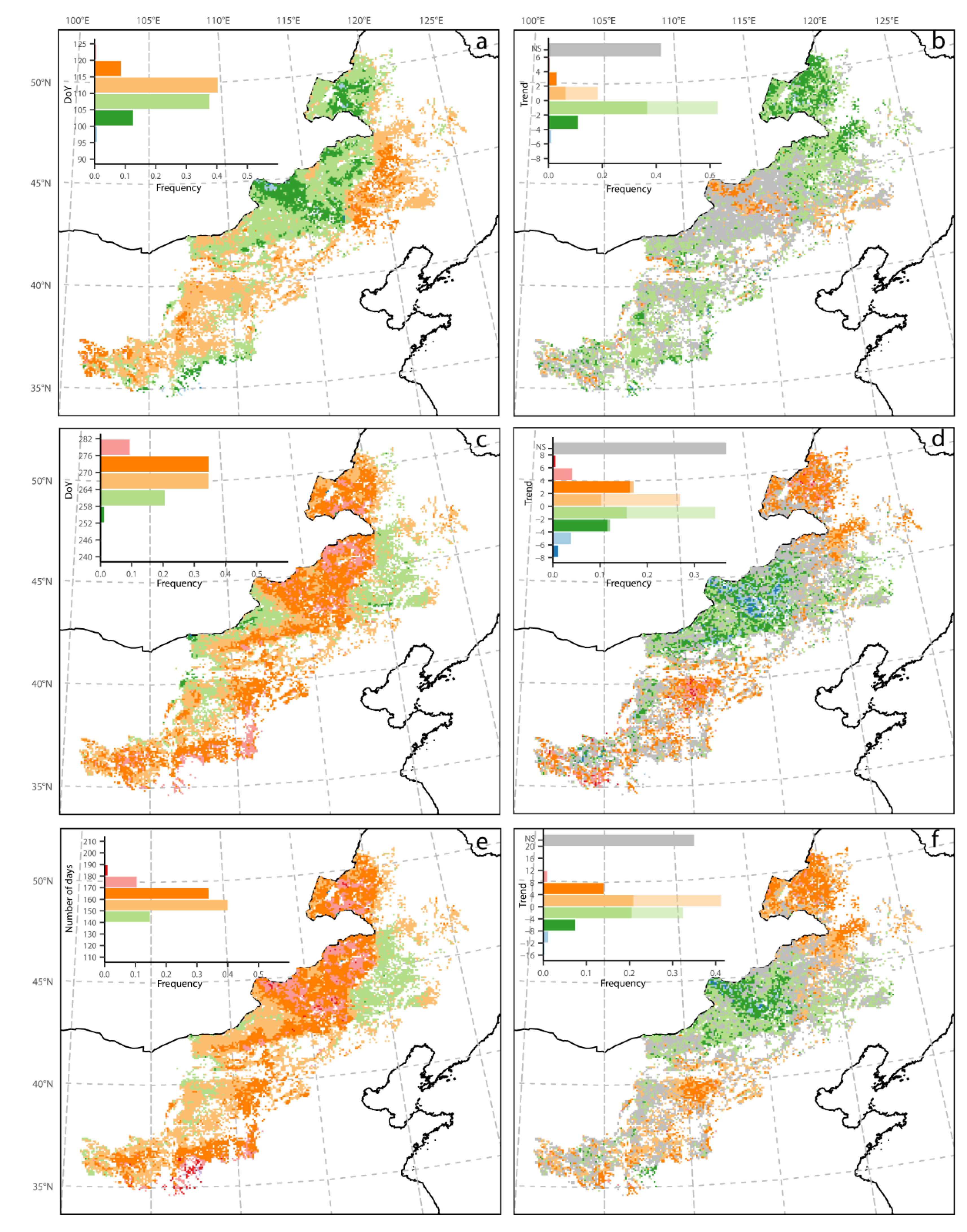
3.2. Spatial Pattern of Phenology Trend and NPP

Between 1982 and 2015, for SOS, about 76% of the pixels showed a decreasing trend, which indicates advanced SOS (with 47% of the whole study area significantly decreasing), while the increasing trend of about 24% of the pixels indicates a delayed SOS (with 9.5% significant increase) (Figure 4b). Thus, the SOS with significant changes accounted for approximately 56.5% of the pixels over the study area, and the rest of the area showed no significant trend. Furthermore, in this significantly changed area, the mean dates of the SOS advanced at an average rate of 1.52 ± 1.04 (mean ± sd) d/decade, which mainly occurred in Hulunbuir, northeast of Xilin Gol, and south of the study area. A delayed SOS by an average rate of 1.45 ± 1.03 d/decade was extensively observed in the central region of Xilin Gol, Chifeng.

For EOS (Figure 4d), about 49.3% (with 32.2% pixels significant) experienced a decreasing trend (advanced EOS), and 50.3% (with 30.6% pixels significant) showed an increasing trend. Thus, both types of significant changes accounted for approximately 62.8% of the study area over the past 34 years. The EOS trend’s spatial pattern was generally opposite to the SOS pattern: The north and south parts of the study area showed an increasing trend, while the middle part showed a decreasing trend. The average change rates of the significantly delayed and advanced trends were 2.72 ± 1.72 d/decade and 2.52 ± 1.69 d/decade, respectively.

Because the spatial patterns of the SOS and EOS trends were in the opposite direction of the patterns that advanced to the SOS area and were broadly consistent with the delayed EOS area, and because the delayed SOS area was broadly consistent with advanced EOS, the variable of LOS was intensified. Indeed, the LOS spatial pattern was similar to that of EOS, and the trend rate was more dramatic (Figure 4f). The mean significant increasing and decreasing trends were 3.92 ± 1.83 d/decade and 3.23 ± 2.38 d/decade, respectively. The NPP spatial pattern can be divided into three parts based on the trends of LOS: The northern region (i.e., the Hulunbuir area), the middle region, including Xilin Gol, Hanshandak, and Ulanqab (i.e., between 41° and 46°N), and the southern region (i.e., south of 46° N). Compared with the other two parts, almost all the pixels of the Hulunbuir region exhibited opposite trends of NPP and LOS, where the NPP was negative and the LOS was positive (Figure 5b). In most pixels in the other two regions, the NPP trends were consistent with the LOS trend in which the middle region was negative, and the south was positive.

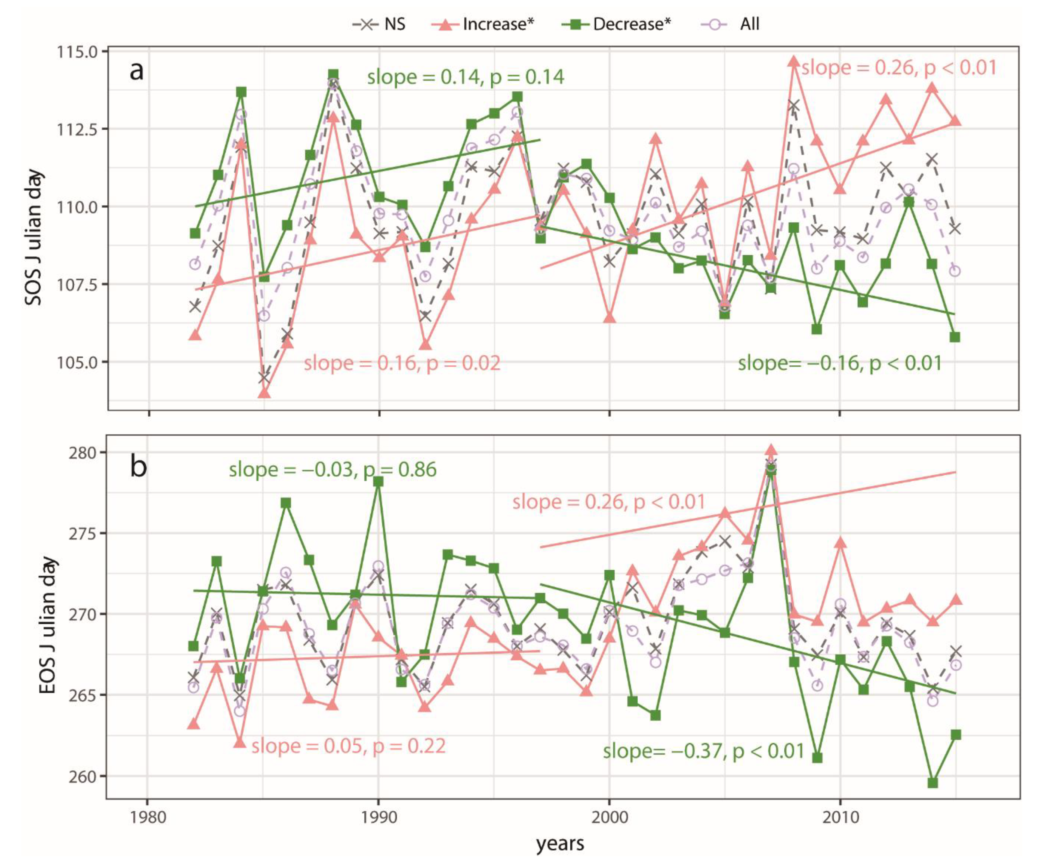
3.3. Phenology Trends over Different Trend Zones

The previous Section 3.2 exhibited the spatial distribution of three types of trends: A significant increase, a significant decrease, and an insignificant change. To further understand the characteristics of temporal change, we present the interannual variation of the different trend zones (Figure 6). Through piecewise regression, we determined that the turning point occurred around 1997.

Figure 6a depicts the interannual SOS variation of each region from 1982 to 2015. The whole area showed a slightly significantly decreasing trend (−0.067 d/decade, p < 0.05, not marked in the figure). Notably, the increasing trend’s SOS (green line) occurred earlier than the decreasing trend’s SOS before 1997, but was later after 1997. Hence, taking 1997 as the break point, we divided the temporal variation into two periods and used linear regression for both significantly changed regions. Overall, the interannual SOS changed significantly before 1997 and with less volatility after 1997. Both SOS trends displayed a weak increase with almost the same slope (slope = 0.14 and 0.16, p < 0.01) before 1997. However, the decreasing region exhibited a descending trend, and the increasing region exhibited a relatively fast increase (slope = −0.16 and 0.26, p < 0.01, respectively).

The EOS interannual variation was similar to the SOS, which showed a higher average for the decreasing region than the increasing region before 2000, which reversed after 2000. Both the increasing and decreasing regions experienced no significant trends before 1997 (slope = −0.03 and 0.05, p = 0.86, and 0.22, respectively), but showed significant trends after 1997 (slope = −0.37 and 0.26, p < 0.01, respectively). Unlike SOS, the whole area showed no significant trend (Figure 6b).

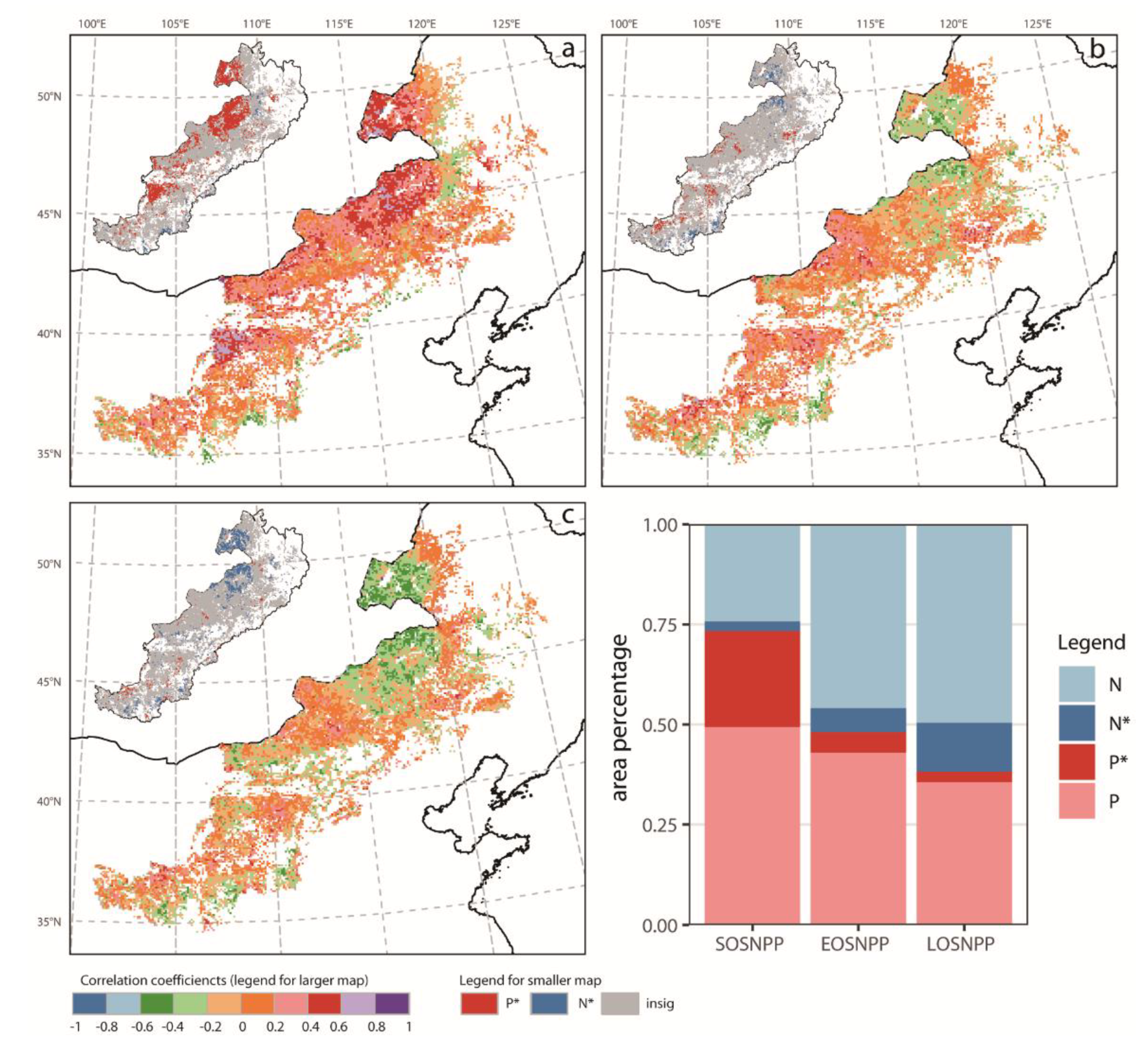
3.4. Quantitative Relationships between NPP and Phenology

A temporal correlation analysis between phenology and NPP was performed at each pixel over the study area. Figure 7a presents the spatial distribution of the correlation between SOS and annual NPP. The majority of pixels exhibit positive correlations, accounting for 74.2% of the area, suggesting that a delayed SOS generally caused an incremental NPP in the current year, and vice versa; therein, the significant correlation pixels were almost positive (24% of the total pixels were significant) and mainly occurred in the north of the study area, such as the west of Hulunbuir and the northeast of Xilin Gol. Compared with SOS, there was a strong spatial heterogeneity throughout the whole area for the relationship between EOS and annual NPP (Figure 7b). The number of positive and negative pixels were almost equal and were scattered throughout the whole region, and the same was true for the significant region (5.2% and 6.0%, respectively). The significant negative pixels scattered in the northern part and southern edge of the study area were significantly positive in the middle. The pattern of the significant correlation between LOS and NPP is similar to that of EOS and NPP, but the northern negative area appears more collective (Figure 7c).

4. Discussion

4.1. Phenology Spatial Pattern and Changes

In this study, we revealed the spatial patterns of phenology (SOS, EOS, LOS) in the northern temperate grasslands of China, which exhibit spatial heterogeneity across the entire study area (Figure 4). The overall spatial distributions of the annual mean SOS and EOS are generally consistent with the in situ observations [42] and other satellite monitors [6,43]; however, some results with regional characteristics were obtained over a long-term period (i.e., 1982–2015). Many studies have reported the earlier tendency of SOS or delayed EOS in various regions of the world under global climate change, with the special characteristic of rising temperature [1,44,45,46,47]. Liu and Piao [48,49] suggested that the average SOS in the entire northern hemisphere advanced with a weak trend of 2.1 d/decade over the period 1982–2011. However, the spatial patterns of these trends were heterogeneous, with a 75% advanced area and a 25% delayed area. In our study area, the average advanced SOS trends were less than those of the entire northern hemisphere, but the northern part of the study area displayed a relatively higher trend, and the clustered delayed SOS region was mainly located in Xilin Gol. This situation was determined via in situ observation. Liu [50] and Wang [51] revealed that the divergent directions of grassland phenological changes under climate change and the SOS of dominant species grass in Xilinhot showed a significant delayed trend during 1982–2011.

The trends in both the SOS and EOS of the whole region appeared to weakly advance during 1982–2015. These results are consistent with previous studies on the changes of phenology in the Mongolian region [52,53]. Through piecewise linear regression on the different regions of change for SOS and EOS, we found that a dramatic trend for grassland phenology emerged around 1997, while there was no obvious trend previously observed. The turning point for the different regions’ trends (increases and decreases) occurred around 1997, which agrees with the changes of phenology in middle and eastern Eurasia [54]. Subsequently, continuous trends in the opposite directions reversed the average SOS/EOS in the different trend regions. This suggests that outstanding changes in phenology will alter the spatial patterns of the phenology. Thus, local phenological change details could be ignored when only checking the trends of the whole area because continuous trends in the opposite directions might offset each other. Phenology depends on vegetation type and other complex environmental factors. A further time-series analysis, which addresses the dynamics of phenology, is challenging because phenology possesses spatial heterogeneity.

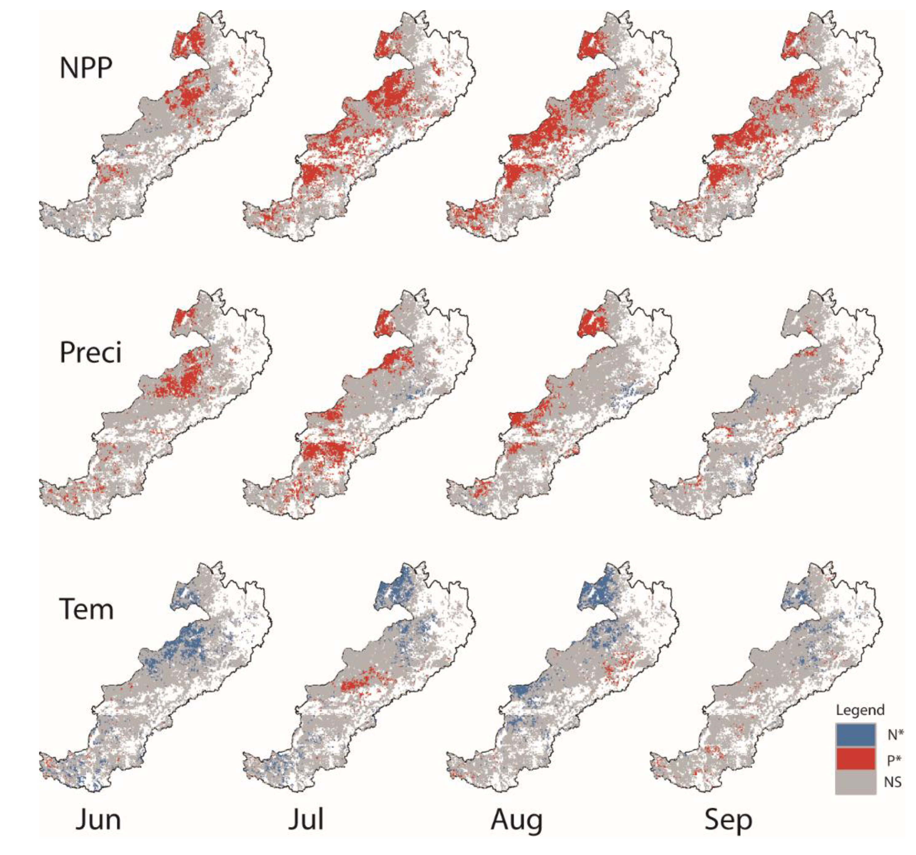
4.2. NPP Response to Phenology

We investigated the relationship between phenology and NPP in the current year and found that among three phenology metrics, the SOS had the closest relation to NPP. SOS experienced the majority of the positive correlation, which means that a delayed SOS indicated a higher NPP in the current year, and vice versa. Compared to SOS, the NPP relationships between EOS and LOS were not as obvious as SOS (Figure 7). Some pixels in the north of the study area exhibited a significant negative correlation between NPP and LOS, which means a higher annual NPP with a shortened LOS. In general, that a prolonged duration of the vegetation’s growing season enhances NPP is conventionally assumed, because more days are possible for photosynthesis and accumulating biomass [5]. Some previous studies confirmed this assumption, showing that NPP increased the coupled growing season length with a rate range of 0.3–1.03% per day on a continental scale [15,17,55,56]. However, some recent studies have provided opposite results that prolonged LOS reduces productivity in some ecosystems, which is attributed to concurrent increases in plant respiration [57,58,59]. In this study, we suggest that the relationship between NPP and LOS illustrates strong regional characteristics.

Phenology and NPP are obviously influenced by meteorological environmental factors, such as temperature, precipitation, and solar radiation (among which temperature and precipitation were considered the most important and were chosen as variables to explore vegetation growth because radiation is not as important a factor as others). SOS is mainly influenced by preseason weather conditions. In terms of climate, we assumed that SOS delays/advances related to the weather influenced the NPP increase/decrease in the current year’s growing season. Therefore, we further examined the relationship between meteorological factors and SOS. Considering that summer NPP accounts for more than 70% of the annual NPP, while the spring and autumn NPPs account for the remaining proportions [52,60], we checked the relationship between the climate factor and SOS in June, July, August, and September. Notably, the pixels where the SOS significantly positively correlated with precipitation and negatively correlated with temperature in the summer months (June, July, and August) were generally consistent with the pixels where the SOS correlated with NPP (Figure 8). In fact, grassland growth strongly depends on precipitation in arid and semi-arid areas, especially in summer, which is the peak growing time when the temperatures are hottest. However, lower temperatures in the summer benefit grass growth because they reduce evapotranspiration and keep the stomata aperture open for CO₂, while maintaining the adequate enzyme activity required for photosynthesis. This could explain why temperatures exhibited a negative relationship to SOS, while NPP was positive (Figure 8).

Temperature variation influences phenology through multiple pathways [61,62,63,64]. It is generally recognized that temperature increases in spring before SOS causes the effective accumulative temperature to reach seed germination and leaf unfolding ahead of time [64,65]. Meanwhile, photosynthetic uptake is generally temperature limited, and warming can enhanced grass growth and greenness [66,67]. On the contrary, temperature increases in the winter will delay the SOS by weakening the chilling shock effect, which is a requirement of the breaking bud dormancy [62,68]. On the other hand, temperature affects phenology via an indirect pathway, through which the higher temperatures in spring expedite evapotranspiration, causing water stress in arid and semi-arid grassland [69,70]. In this study area, most pixels showed that SOS was positively correlated with the temperature in April, which indicates a higher temperature delayed SOS. This delay is attributed to the higher temperatures resulting in soil water stress. Previous studies have recognized that spring rainfall is the trigger for grassland green-up, which could be evidence of higher temperature restrained SOS. Some meteorological studies revealed that reducing soil moisture to increase surface temperature increases the land–sea temperature gradient and produces a cyclonic anomaly, which enhances the summer monsoon, thereby resulting in more rainfall [71,72]. This could explain why SOS showed a positive correlation with summer precipitation. Thus, although the delayed SOS reduced spring NPP, the growth promoted by sufficient rainfall in the summer can compensate for the loss NPP in spring. Meanwhile, lower temperatures in the summer facilitate grass growth. This result serves as a theoretical guideline for the treatment of grazing planning and the rational utilization of grassland resources.

4.3. Uncertainty and Expectations

Remote sensing-based techniques are able to successfully monitor large-scale ecosystem changes and have been frequently applied in recent years [18,73], but there are some uncertainties along with the data management in this study. GIMMS datasets possess long-time-series observation records for land surface changes as a benefit, but their rough spatial resolution (0.5 degree, about 8 km) is too large to match the field investigation because vegetation phenology varies with vegetation type and soil texture, even in an 8 km-pixel area. In addition, there is a lack of long time-series stable ground observations of phenology for the whole study area, thereby preventing us from setting a suitable targeted threshold for different grassland regions. These constraints have forced us to calculate the phenology by the sole threshold value. However, the data of the threshold method may not completely match those of conventional field-observed phenological events, but rather express indicators of vegetation greenness dynamics [74]. From this perspective, SOS estimation is relatively more accurate than EOS when using the threshold method, because grassland vegetation maintains a certain level of greenness, even when the growth has stopped at the senescence phase [75]. Recent studies reported that EOS may make more contribution than SOS to prolonging/shortening the growing season length, which highlights the need to model EOS. Thus, there are several ways to improve the accuracy of vegetation phenology extraction: A field investigation corresponding with high resolution satellite sensors, such as Moderate Resolution Imaging Spectroradiometer (MODIS), with a 1 km or 500 m resolution, fused with a rough resolution NDVI [76]; or gathering the best threshold for the targeted region and applying different thresholds in different zones, so the NDVI phenology of the whole area will be more accurate.

5. Conclusions

In this study, using GIMMS-3g NDVI and meteorological data, we detected the spatial pattern and changes in phenology and NPP from 1982 to 2015 on the temperate grassland of China, and further investigated interannual variation and trends. Then, we analyzed the relationship between the NPP and phenological dynamics on a spatial scale. More than half of the study area displayed significant changes in the phenology and NPP over the past 34 years, and the trends exhibited spatial heterogeneity. Based on examining the interannual variations of the different trends’ pixels, we found that the phenology presented obvious trends after 1997, while no significant changes were found previously. The SOS correlated strongly with the NPP during the same year, especially in the drought inland area, because a drought-caused delayed SOS is always associated with a strong summer monsoon, which produces greater precipitation in summer. Therefore, SOS is an important indicator to predict the current year’s NPP, which provides a reference for local pasture husbandry.

References

1. Menzel, A. Trends in phenological phases in Europe between 1951 and 1996. Int. J. Biometeorol. 2000, 44, 76–81. [Google Scholar] [CrossRef] [PubMed]
2. IPCC. Climate Change 2013: The Physical Science Basis; Cambridge University Press: Cambridge, UK, 2013. [Google Scholar]
3. Hayden, B.P. Ecosystem feedbacks on climate at the landscape scale. Philos. Trans. R. Soc. Lond. B. Biol. Sci. 1998, 353, 5–18. [Google Scholar] [CrossRef] [Green Version]
4. Hogg, E.H.; Price, D.T.; Black, T.A. Postulated feedbacks of deciduous forest phenology on seasonal climate patterns in the western Canadian interior. J. Clim. 2000, 13, 4229–4243. [Google Scholar] [CrossRef]
5. Richardson, A.D.; Black, A.T.; Ciais, P.; Delbart, N.; Friedl, M.A.; Nadine, G.; Hollinger, D.Y.; Kutsch, W.L.; Bernard, L.; Sebastiaan, L.; et al. Influence of spring and autumn phenological transitions on forest ecosystem productivity. Philos. Trans. R. Soc. B Biol. Sci. 2010, 365, 3227–3246. [Google Scholar] [CrossRef] [PubMed] [Green Version]
6. Jeong, S.-J.; Ho, C.-H.; Gim, H.-J.; Brown, M.E. Phenology shifts at start vs. end of growing season in temperate vegetation over the Northern Hemisphere for the period 1982–2008. Glob. Chang. Biol. 2011, 17, 2385–2399. [Google Scholar] [CrossRef]
7. Ren, S.; Chen, X.; Lang, W.; Schwartz, M.D. Climatic controls of the spatial patterns of vegetation phenology in midlatitude grasslands of the Northern Hemisphere. J. Geophys. Res. Biogeosci. 2018, 123, 2323–2336. [Google Scholar] [CrossRef]
8. Zheng, D.L.; Prince, S.; Wright, R. Terrestrial net primary production estimates for 0.5° grid cells from field observations—A contribution to global biogeochemical modeling. Glob. Chang. Biol. 2003, 9, 46–64. [Google Scholar] [CrossRef]
9. Clark, D.A.; Brown, S.; Kicklighter, D.W.; Chambers, J.Q.; Thomlinson, J.R.; Ni, J. Measuring net primary production in forests: concepts and field methods. Ecol. Appl. 2001, 11, 356–370. [Google Scholar] [CrossRef]
10. Bernacki, Z. Biomass production of maize (Zea mays L.) cropping in exceptionally advantageous conditions in central Wielkopolska (Poland). Biomass Bioenergy 2018, 110, 25–32. [Google Scholar] [CrossRef]
11. Prince, S.D.; Haskett, J.; Steininger, M.; Strand, H.; Wright, R. Net primary production of US Midwest croplands from agricultural harvest yield data. Ecol. Appl. 2001, 11, 1194–1205. [Google Scholar] [CrossRef]
12. Scurlock, J.M.O.; Johnson, K.; Olson, R.J. Estimating net primary productivity from grassland biomass dynamics measurements. Glob. Chang. Biol. 2002, 8, 736–753. [Google Scholar] [CrossRef] [Green Version]
13. Tang, G.; Beckage, B.; Smith, B.; Miller, P.A. Estimating potential forest NPP, biomass and their climatic sensitivity in New England using a dynamic ecosystem model. Ecosphere 2010, 1, 1–20. [Google Scholar] [CrossRef] [Green Version]
14. Zhao, M.; Zhou, G.S. Estimation of biomass and net primary productivity of major planted forests in China based on forest inventory data. For. Ecol. Manag. 2005, 207, 295–313. [Google Scholar] [CrossRef]
15. Nemani, R.R. Climate-driven increases in global terrestrial net primary production from 1982 to 1999. Science 2003, 300, 1560–1563. [Google Scholar] [CrossRef] [PubMed] [Green Version]
16. Falge, E.; Baldocchi, D.; Tenhunen, J.; Aubinet, M.; Bakwin, P.; Berbigier, P.; Bernhofer, C.; Burba, G.; Clement, R.; Davis, K.J.; et al. Seasonality of ecosystem respiration and gross primary production as derived from FLUXNET measurements. Agric. For. Meteorol. 2002, 113, 53–74. [Google Scholar] [CrossRef] [Green Version]
17. Piao, S.; Friedlingstein, P.; Ciais, P.; Viovy, N.; Demarty, J. Growing season extension and its impact on terrestrial carbon cycle in the Northern Hemisphere over the past 2 decades. Glob. Biogeochem. Cycles 2007, 21, GB3018. [Google Scholar] [CrossRef]
18. White, M.A.; De Beurs, K.M.; Didan, K.; Inouye, D.W.; Richardson, A.D.; Jensen, O.P.; O’Keefe, J.; Zhang, G.; Nemani, R.R.; Van Leeuwen, W.J.D.; et al. Intercomparison, interpretation, and assessment of spring phenology in North America estimated from remote sensing for 1982–2006. Glob. Chang. Biol. 2009, 15, 2335–2359. [Google Scholar] [CrossRef]
19. Wang, S.; Zhang, B.; Yang, Q.; Chen, G.; Yang, B.; Lu, L.; Shen, M.; Peng, Y. Responses of net primary productivity to phenological dynamics in the Tibetan Plateau, China. Agric. For. Meteorol. 2017, 232, 235–246. [Google Scholar] [CrossRef]
20. Wu, C.; Hou, X.; Peng, D.; Gonsamo, A.; Xu, S. Land surface phenology of China’s temperate ecosystems over 1999–2013: Spatial–temporal patterns, interaction effects, covariation with climate and implications for productivity. Agric. For. Meteorol. 2016, 216, 177–187. [Google Scholar] [CrossRef]
21. Conventry, D. World Resources 2000–2001: People and Ecosystems—The Fraying Web of Life. Agric. Ecosyst. Environ. 2001, 86, 109–110. [Google Scholar] [CrossRef]
22. Kang, L.; Han, X.; Zhang, Z.; Sun, O.J. Grassland ecosystems in China: Review of current knowledge and research advancement. Philos. Trans. R. Soc. B Biol. Sci. 2007, 362, 997–1008. [Google Scholar] [CrossRef] [PubMed]
23. Chinese Academy of Sciences. Vegetation Atlas of China; Science Press: Beijing, China, 2001. [Google Scholar]
24. Pinzon, J.; Tucker, C. A non-stationary 1981–2012 AVHRR NDVI3g time series. Remote Sens. 2014, 6, 6929–6960. [Google Scholar] [CrossRef] [Green Version]
25. Hutchinson, M.F.; Dan, M.K.; Lawrence, K.; Pedlar, J.H.; Hopkinson, R.F.; Milewska, E.; Papadopol, P. Development and testing of Canada-wide interpolated spatial models of daily minimum–maximum temperature and precipitation for 1961–2003. J. Appl. Meteorol. Clim. 2010, 48, 725–741. [Google Scholar] [CrossRef]
26. Viovy, N.; Arino, O.; Belward, A.S. The Best Index Slope Extraction (BISE): A method for reducing noise in NDVI time-series. Int. J. Remote Sens. 1992, 13, 1585–1590. [Google Scholar] [CrossRef]
27. Chen, J.; Joönsson, P.; Tamura, M.; Gu, Z.; Matsushita, B.; Eklundh, L. A simple method for reconstructing a high-quality NDVI time-series data set based on the Savitzky-Golay filter. Remote Sens. Environ. 2004, 91, 332–344. [Google Scholar] [CrossRef]
28. Beck, P.S.A.; Atzberger, C.; Høgda, K.A.; Johansen, B.; Skidmore, A.K. Improved monitoring of vegetation dynamics at very high latitudes: A new method using MODIS NDVI. Remote Sens. Environ. 2006, 100, 321–334. [Google Scholar] [CrossRef]
29. White, M.A.; Thornton, P.E.; Running, S.W. A continental phenology model for monitoring vegetation responses to interannual climatic variability. Glob. Biogeochem. Cycles 1997, 11, 217–234. [Google Scholar] [CrossRef]
30. Guo, J.; Yang, X.; Niu, J.; Jin, Y.; Xu, B.; Shen, G.; Zhang, W.; Zhao, F.; Zhang, Y. Remote sensing monitoring of green-up dates in the Xilingol grasslands of northern China and their correlations with meteorological factors. Int. J. Remote Sens. 2019, 40, 2190–2211. [Google Scholar] [CrossRef]
31. Zhao, J.; Zhang, H.; Zhang, Z.; Guo, X.; Li, X.; Chen, C. Spatial and temporal changes in vegetation phenology at middle and high latitudes of the Northern Hemisphere over the past three decades. Remote Sens. 2015, 7, 10973–10995. [Google Scholar] [CrossRef] [Green Version]
32. Bao, G.; Bao, Y.; Qin, Z.; Xin, X.; Bao, Y.; Bayarsaikan, S.; Zhou, Y.; Chuntai, B. Modeling net primary productivity of terrestrial ecosystems in the semi-arid climate of the Mongolian Plateau using LSWI-based CASA ecosystem model. Int. J. Appl. Earth Obs. Geoinf. 2016, 46, 84–93. [Google Scholar] [CrossRef]
33. Liu, C.; Dong, X.; Liu, Y. Changes of NPP and their relationship to climate factors based on the transformation of different scales in Gansu, China. Catena 2015, 125, 190–199. [Google Scholar] [CrossRef]
34. Nayak, R.K.; Patel, N.R.; Dadhwal, V.K. Inter-annual variability and climate control of terrestrial net primary productivity over India. Int. J. Clim. 2013, 33, 132–142. [Google Scholar] [CrossRef]
35. Yu, D.Y.; Shi, P.J.; Shao, H.B.; Zhu, W.Q.; Pan, Y.H. Modelling net primary productivity of terrestrial ecosystems in East Asia based on an improved CASA ecosystem model. Int. J. Remote Sens. 2009, 30, 4851–4866. [Google Scholar] [CrossRef]
36. Potter, S.; Randerson, T.; Field, B.; Matson, A.; Mooney, H.A. Terrestrial ecosystem production: A process model based on global satellite and surface data. 1993, 7, 811–841. [Google Scholar] [CrossRef]
37. Zhang, M.; Lal, R.; Zhao, Y.; Jiang, W.; Chen, Q. Estimating net primary production of natural grassland and its spatio-temporal distribution in China. Sci. Total Environ. 2016, 553, 184–195. [Google Scholar] [CrossRef]
38. Sen, P.K. Estimates of the regression coefficient based on Kendall’s tau. J. Am. Stat. Assoc. 1968, 63, 1379–1389. [Google Scholar] [CrossRef]
39. Theil, H. A rank-invariant method of linear and polynomial regression analysis. Henri Theil’s Contrib. Econ. Econometr. 1950, 345–381. [Google Scholar]
40. Toms, J.D.; Lesperance, M.L. Piecewise regression: A tool for identifying ecological thresholds. Ecology 2003, 84, 2034–2041. [Google Scholar] [CrossRef]
41. Chang, Q.; Zhang, J.; Jiao, W.; Yao, F.; Wang, S. Spatiotemporal dynamics of the climatic impacts on greenup date in the Tibetan Plateau. Environ. Earth Sci. 2016, 75, 1343. [Google Scholar] [CrossRef]
42. Chen, X.; Li, J.; Xu, L.; Liu, L.; Ding, D. Modeling greenup date of dominant grass species in the Inner Mongolian Grassland using air temperature and precipitation data. Int. J. Biometeorol. 2014, 58, 463–471. [Google Scholar] [CrossRef]
43. Zhang, T.; Zhang, Y.; Xu, M.; Xi, Y.; Zhu, J.; Zhang, X.; Wang, Y.; Li, Y.; Shi, P.; Yu, G.; et al. Ecosystem response more than climate variability drives the inter-annual variability of carbon fluxes in three Chinese grasslands. Agric. For. Meteorol. 2016, 225, 48–56. [Google Scholar] [CrossRef]
44. Defila, C.; Clot, B. Phytophenological trends in Switzerland. Int. J. Biometeorol. 2001, 45, 203–207. [Google Scholar] [CrossRef] [PubMed]
45. Gordo, O.; Sanz, J.J. Impact of climate change on plant phenology in Mediterranean ecosystems. Glob. Chang. Biol. 2010, 16, 1082–1106. [Google Scholar] [CrossRef]
46. Piao, S.; Fang, J.; Zhou, L.; Ciais, P.; Zhu, B. Variations in satellite-derived phenology in China’s temperate vegetation. Glob. Chang. Biol. 2006, 12, 672–685. [Google Scholar] [CrossRef]
47. Pierre, C.; Grippa, M.; Mougin, E.; Guichard, F.; Kergoat, L. Changes in Sahelian annual vegetation growth and phenology since 1960: A modeling approach. Glob. Planet. Chang. 2016, 143, 162–174. [Google Scholar] [CrossRef]
48. Liu, Q.; Fu, Y.H.; Zhu, Z.; Liu, Y.; Liu, Z.; Huang, M.; Janssens, I.A.; Piao, S. Delayed autumn phenology in the Northern Hemisphere is related to change in both climate and spring phenology. Glob. Chang. Biol. 2016, 22, 3702–3711. [Google Scholar] [CrossRef]
49. Piao, S.; Liu, Q.; Chen, A.; Janssens, I.A.; Fu, Y.; Dai, J.; Liu, L.; Lian, X.; Shen, M.; Zhu, X. Plant phenology and global climate change: Current progresses and challenges. Glob. Chang. Biol. 2019, 25, 1922–1940. [Google Scholar] [CrossRef]
50. Liu, H.; Tian, F.; Hu, H.C.; Hu, H.P.; Sivapalan, M. Soil moisture controls on patterns of grass green-up in Inner Mongolia: An index based approach. Hydrol. Earth Syst. Sci. 2013, 17, 805–815. [Google Scholar] [CrossRef] [Green Version]
51. Wang, G.; Huang, Y.; Wei, Y.; Zhang, W.; Li, T.; Zhang, Q. Inner Mongolian grassland plant phenological changes and their climatic drivers. Sci. Total Environ. 2019, 683, 1–8. [Google Scholar] [CrossRef]
52. Bao, G.; Chen, J.; Chopping, M.; Bao, Y.; Bayarsaikhan, S.; Dorjsuren, A.; Tuya, A.; Jirigala, B.; Qin, Z. Dynamics of net primary productivity on the Mongolian Plateau: Joint regulations of phenology and drought. Int. J. Appl. Earth Obs. Geoinf. 2019, 81, 85–97. [Google Scholar] [CrossRef]
53. Kang, W.; Wang, T.; Liu, S. The response of vegetation phenology and productivity to drought in semi-arid regions of Northern China. Remote Sens. 2018, 10, 727. [Google Scholar] [CrossRef] [Green Version]
54. Li, Y.; Zhang, Y.; Gu, F.; Liu, S. Discrepancies in vegetation phenology trends and shift patterns in different climatic zones in middle and eastern Eurasia between 1982 and 2015. Ecol. Evol. 2019, 9. [Google Scholar] [CrossRef] [PubMed] [Green Version]
55. Fang, J.; Piao, S.; Field, C.B.; Pan, Y.; Guo, Q.; Zhou, L.; Peng, C.; Tao, S. Increasing net primary production in China from 1982 to 1999. Front. Ecol. Environ. 2003, 1, 293–297. [Google Scholar] [CrossRef]
56. Hicke, J.A.; Asner, G.P.; Randerson, J.T.; Tucker, C.; Los, S.; Birdsey, R.; Jenkins, J.C.; Field, C.; Holland, E. Satellite-derived increases in net primary productivity across North America, 1982–1998. Geophys. Res. Lett. 2002, 29. [Google Scholar] [CrossRef] [Green Version]
57. Dunn, A.L.; Barford, C.C.; Wofsy, S.C.; Goulden, M.L.; Daube, B.C. A long-term record of carbon exchange in a boreal black spruce forest: Means, responses to interannual variability, and decadal trends. Glob. Chang. Biol. 2007, 13, 577–590. [Google Scholar] [CrossRef] [Green Version]
58. Piao, S.; Ciais, P.; Friedlingstein, P.; Peylin, P.; Reichstein, M.; Luyssaert, S.; Margolis, H.; Fang, J.; Barr, A.; Chen, A.; et al. Net carbon dioxide losses of northern ecosystems in response to autumn warming. Nature 2008, 451, 49. [Google Scholar] [CrossRef]
59. Sacks, W.J.; Schimel, D.S.; Monson, R. Coupling between carbon cycling and climate in a high-elevation, subalpine forest: A model-data fusion analysis. Oecologia 2007, 151, 54–68. [Google Scholar] [CrossRef]
60. Sui, X.; Zhou, G.; Zhuang, Q. Sensitivity of carbon budget to historical climate variability and atmospheric CO2 concentration in temperate grassland ecosystems in China. Clim. Chang. 2013, 117, 259–272. [Google Scholar] [CrossRef]
61. Lin, S.; Shao, L.; Hui, C.; Sandhu, H.S.; Fan, T.; Zhang, L.; Li, F.; Ding, Y.; Shi, P. The effect of temperature on the developmental rates of seedling emergence and leaf-unfolding in two dwarf bamboo species. Trees 2018, 32, 751–763. [Google Scholar] [CrossRef]
62. Martiínez-Luüscher, J.; Hadley, P.; Ordidge, M.; Xu, X.; Luedeling, E. Delayed chilling appears to counteract flowering advances of apricot in southern UK. Agric. For. Meteorol. 2017, 237–238, 209–218. [Google Scholar]
63. Pope, K.S.; Da Silva, D.; Brown, P.H.; DeJong, T.M. A biologically based approach to modeling spring phenology in temperate deciduous trees. Agric. For. Meteorol. 2014, 198–199, 15–23. [Google Scholar] [CrossRef]
64. Shi, P.; Chen, Z.; Reddy, G.V.P.; Hui, C.; Huang, J.; Xiao, M. Timing of cherry tree blooming: Contrasting effects of rising winter low temperatures and early spring temperatures. Agric. For. Meteorol. 2017, 240–241, 78–89. [Google Scholar] [CrossRef] [Green Version]
65. Harrington, C.A.; Gould, P.J. Tradeoffs between chilling and forcing in satisfying dormancy requirements for Pacific Northwest tree species. Front. Plant Sci. 2015, 6. [Google Scholar] [CrossRef] [PubMed] [Green Version]
66. Lucht, W.; Prentice, I.C.; Myneni, R.B.; Sitch, S.; Friedlingstein, P.; Cramer, W.; Bousquet, P.; Buermann, W.; Smith, B. Climatic control of the high-latitude vegetation greening trend and Pinatubo effect. Science 2002, 296, 1687–1689. [Google Scholar] [CrossRef] [PubMed] [Green Version]
67. Tanja, S.; Berninger, F.; Vesala, T.; Markkanen, T.; Hari, P.; Mäkelä, A.; Ilvesniemi, H.; Hänninen, H.; Nikinmaa, E.; Huttula, T.; et al. Air temperature triggers the recovery of evergreen boreal forest photosynthesis in spring. Glob. Chang. Biol. 2003, 9, 1410–1426. [Google Scholar] [CrossRef]
68. Vitasse, Y.; Lenz, A.; Körner, C. The interaction between freezing tolerance and phenology in temperate deciduous trees. Front. Plant Sci. 2014, 5, 541. [Google Scholar] [CrossRef] [Green Version]
69. Knapp, A.K.; Beier, C.; Briske, D.D.; Classen, A.T.; Luo, Y.; Reichstein, M.; Smith, M.D.; Smith, S.D.; Bell, J.E.; Fay, P.A.; et al. Consequences of more extreme precipitation regimes for terrestrial ecosystems. BioScience 2008, 58, 811–821. [Google Scholar] [CrossRef]
70. Shen, W.; Jenerette, G.D.; Hui, D.; Phillips, R.P.; Ren, H. Effects of changing precipitation regimes on dryland soil respiration and C pool dynamics at rainfall event, seasonal and interannual scales. J. Geophys. Res. Biogeosci. 2008, 113. [Google Scholar] [CrossRef]
71. Grimm, A.M.; Pal, J.S.; Giorgi, F. Connection between spring conditions and peak summer monsoon rainfall in South America: Role of soil moisture, surface temperature, and topography in eastern Brazil. J. Clim. 2007, 20, 5929–5945. [Google Scholar] [CrossRef] [Green Version]
72. Zuo, Z.; Zhang, R. The spring soil moisture and the summer rainfall in eastern China. Chin. Sci. Bull. 2007, 52, 3310–3312. [Google Scholar] [CrossRef]
73. Xin, Q.; Broich, M.; Zhu, P.; Gong, P. Modeling grassland spring onset across the Western United States using climate variables and MODIS-derived phenology metrics. Remote Sens. Environ. 2015, 161, 63–77. [Google Scholar] [CrossRef]
74. Reed, B.C.; Brown, J.F.; VanderZee, D.; Loveland, T.R.; Merchant, J.W.; Ohlen, D.O. Measuring phenological variability from satellite imagery. J. Veg. Sci. 1994, 5, 703–714. [Google Scholar] [CrossRef]
75. Fridley, J.D. Extended leaf phenology and the autumn niche in deciduous forest invasions. Nature 2012, 485, 359–362. [Google Scholar] [CrossRef] [PubMed]
76. Tian, F.; Wang, Y.; Fensholt, R.; Wang, K.; Zhang, L.; Huang, Y. Mapping and evaluation of NDVI trends from synthetic time series obtained by blending Landsat and MODIS data around a coalfield on the Loess Plateau. Remote Sens. 2013, 5, 4255–4279. [Google Scholar] [CrossRef] [Green Version]
Figure 1. The spatial distribution of grassland vegetation in the temperate grassland zone of China.
Sustainability 12 00012 g001
Figure 2. Method for Savitzky–Golay filtering (SG) and retrieving the start (SOS) and end (EOS) of the growing season dates based on the normalized difference vegetation index (NDVI) time series.
Sustainability 12 00012 g002
Figure 3. Comparisons between modeled and field-observed SOS (a); EOS (b); and net primary productivity (NPP) (c).
Sustainability 12 00012 g003
Figure 4. Spatial patterns of phenological metrics, trends, and pixel value frequencies over temperate grasslands during 1983–2015. (a) The mean Julian day of the SOS; (b) the trend of SOS (d/decade); (c) the mean Julian day of EOS; (d) the trend of EOS (d/decade); (e) the mean Julian day of length of the growing season (LOS); and (f) the trend of LOS (d/decade). Note: DoY indicates the Julian day of the year; NS indicates nonsignificant; the translucent bar indicates the insignificant part.
Sustainability 12 00012 g004
Figure 5. Spatial patterns of the average NPP (a) and time-series trends (b) over temperate grasslands during 1983–2015. Note: NS indicates nonsignificant; the barplot indicates the pixel value frequency; the translucent bars indicate insignificant parts.
Sustainability 12 00012 g005
Figure 6. Interannual variations of the different trend zones of SOS (a) and EOS (b) in the temperate grasslands of China for 1982–2015. Note: NS indicates insignificantly changed zones; Increase* indicates significantly increased (delayed) zones; Decrease* indicates significantly decreased (advanced) zones; All indicates the whole area.
Sustainability 12 00012 g006
Figure 7. The correlation coefficients between SOS (a); EOS (b); LOS (c); and NPP; barplot counting the pixels of different relations. Note: p indicates a positive relation; N indicates a negative relation; an asterisk (*) indicates significance with a confidence of 95% (p < 0.05).
Sustainability 12 00012 g007
Figure 8. The spatial distribution of the significant relationship between SOS and NPP, precipitation (Preci), and temperature (Tem) for June, July, August, and September. Note: p indicates positive relation; N indicates a negative relation; asterisk (*) indicates significant with a confidence of 95% (p < 0.05).
Sustainability 12 00012 g008