Article

Development of a Biogeochemical and Carbon Model Related to Ocean Acidification Indices with an Operational Ocean Model Product in the North Western Pacific

1
Application Laboratory, Japan Agency for Marine-Earth Science and Technology, 3173-25, Showa-machi, Kanazawa-ku, Yokohama-city, Kanagawa 236-0001, Japan
2
Ocean Policy Research Institute, Sasakawa Peace Foundation, 1-15-16 Toranomon, Minato-ku, Tokyo 105-0001, Japan
3
Center for Marine Environmental Studies, Ehime University, 2-5, Bunkyo-ku, Matsuyama, Ehime 790-8577, Japan
*
Author to whom correspondence should be addressed.
Sustainability 2019, 11(9), 2677; https://doi.org/10.3390/su11092677
Submission received: 28 February 2019 / Revised: 30 April 2019 / Accepted: 6 May 2019 / Published: 10 May 2019

Abstract

:
We developed a biogeochemical and carbon model (JCOPE_EC) coupled with an operational ocean model for the North Western Pacific. JCOPE_EC represents ocean acidification indices on the background of the risks due to ocean acidification and our model experiences. It is an off-line tracer model driven by a high-resolution regional ocean general circulation model (JCOPE2M). The results showed that the model adequately reproduced the general patterns in the observed data, including the seasonal variability of chlorophyll-a, dissolved inorganic nitrogen/phosphorus, dissolved inorganic carbon, and total alkalinity. We provide an overview of this system and the results of the model validation based on the available observed data. Sensitivity analysis using fixed values for temperature, salinity, dissolved inorganic carbon and total alkalinity helped us identify which variables contributed most to seasonal variations in the ocean acidification indices, pH and Ωarg. The seasonal variation in the pHinsitu was governed mainly by balances of the change in temperature and dissolved inorganic carbon. The seasonal increase in Ωarg from winter to summer was governed mainly by dissolved inorganic carbon levels.

1. Introduction

Ocean acidification poses a serious risk to marine organisms and ecosystems, including finfish and coral reefs in subtropical regions, and species or groups of organisms in polar regions [1,2,3,4,5]. The effects of ocean acidity have previously been reported and the effects of acidification are predicted to increase, with great risks to marine organisms [2,4,5,6,7]. The global economic loss of organisms from ocean acidification has been estimated at $24 billion, $0.7 billion, $37 billion, $65 billion, and $30–375 billion for molluscs, echinoderms, crustaceans, finfish, and corals, respectively. Some organisms including molluscs and echinoderms may become locally extinct, and corals will be damaged by the combined effects of global warming and ocean acidification, which will reduce calcification, increase bio-erosion, and have synergistic effects [8]. All organisms except echinoderms could be seriously affected, and substantial economic losses are likely [8]. Therefore, these issues can no longer be ignored, and urgent action is necessary.
The levels of ocean acidification are evaluated using parameters such as the pH and/or the aragonite saturation (Ωarg). However, there are limited observed data for pH and Ωarg, so it is difficult to assess the current status of ocean acidification both locally and globally [3,9]. This situation is unlikely to change even if new automatic monitoring systems, such as biological profiling floats [10], are established and operational monitoring, using volunteer observing ship (VOS) pCO2 transects [11,12], increases.
Numerical model simulations are important tools that support the interpretation of observed data at the required spatial and temporal scales in a dynamically consistent manner, and are used to characterize the underlying physical–biological processes [13,14,15,16,17]. The term ‘modeling’ describes various processes including those associated with nitrate, phytoplankton, zooplankton, and detritus (NPZD processes), which are connected to the carbon cycle throughout photosynthesis, remineralization, and calcination [18]. These NPZD processes influence ocean acidification indices, so marine carbon and biogeochemical models are useful for understanding past, present, and future ocean acidification.
Biogeochemical models focused on NPZD processes in the North Pacific have been developed by Kawamiya et al. [19,20,21], Kishi et al. [22], Fujii et al. [23], Yoshie et al. [24] and Sasai et al. [25]. Onitsuka and Yanagi [26], Guo and Yanagi [27] and Yoshie et al. [24] have developed biogeochemical models for marginal seas including the Japan Sea, the East China Sea and the Seto Inland Sea, respectively. These models included primary productivity among the NPZD processes, but did not include the carbon cycle. Zhao and Guo [28] established an inorganic carbon system module for the Yellow and East China Seas, and Luo et al. [29] constructed a carbon biogeochemical model using the NORWeigian Ecological Model (NORWECOM) and a hydrodynamic module [28].
Earth System Models (ESMs) are climate models that may include physical processes and biogeochemical cycles, and so can facilitate representation of anthropogenic effects on the carbon cycle. In modeling future scenarios, marine ecosystems in ESMs are adapted to particular environmental conditions based on social and economic scenarios (Coupled Model Intercomparison Project Phase 5; [30,31,32,33,34]). Several modeling studies have used coupled climate–marine biogeochemical models to investigate how environmental stressors might evolve under climate change scenarios [30,34]. While ESMs provide past/present/future distributions of several biogeochemical components, and approximately reproduce the large-scale patterns of the subpolar and subtropical gyres, their outputs are not necessarily adequate for reproducing smaller-scale patterns, including shelf processes and/or mesoscale phenomena.
The Japan Coastal Ocean Predictability Experiment (JCOPE: http://www.jamstec.go.jp/jcope/) is an operational eddy-resolving ocean physical model. The latest version of the model (JCOPE2M) [35,36] assimilates satellite sea surface height anomalies and sea surface temperature, and temperature and salinity data obtained from floating profilers and/or ship measurements. The JCOPE2M covers the marginal seas of Japan (including the Okhotsk, Japan and East China Seas) in the geographic range defined by 10.5°–62° N and 108°–180° E (Figure 1). It reproduces the Kuroshio, Oyashio, mesoscale eddies, and upwelling and mixing, which play crucial roles in biological processes related to primary productivity in the upper ocean. The model products provide reanalysis data based on assimilations of all the available observed data. The model outputs include data on velocities, temperature, salinity, and sea elevation that are corrected using data assimilation techniques, and the model more realistically reproduces the physical conditions than non-operational physical models.
To improve our insights into the drivers of ocean acidification, we aimed to develop the JCOPE further to incorporate a new marine ecosystem and carbon cycle model (hereafter JCOPE_EC), driven by the physical processes represented by the JCOPE2M model outputs [37]. In this contribution, we provide a description of the JCOPE_EC, and report on the quality of the model outputs by comparing them with available observed data. The present version of the JCOPE_EC includes damping terms for the climatological states of dissolved inorganic nitrate (DIN), dissolved inorganic phosphate (DIP), dissolved inorganic carbon (DIC) and total alkalinity (ALK) and so can be used to determine the distributions of ocean acidification indices in the North Western Pacific, with a constraint to the climatological information. Sensitivity analysis was performed using fixed values for temperature, salinity, DIC, and ALK, to assess which variables were important in determining the ocean acidification indices, pH and aragonite saturation (Ωarg).
This is the first time the development of an operational carbon cycle model with eddy-resolving horizontal resolution focused on the North Western Pacific has been reported. Some fundamental data required for our study (e.g., climatology data) had to be acquired because only a few of the necessary data for research in this challenging scientific field were available.
Details of the model formulation are provided in Section 2. The data and model parameters used in the study are described in Section 3. Section 4 describes how the model was validated with observed data. In Section 5, the influence of some environmental variables on ocean acidification indices (pH and Ωarg) are discussed. The main findings of the study are overviewed, and future issues are discussed, in Section 6.

2. Model Formation

The JCOPE_EC was constructed on an offline tracer model driven by physical processes simulated by the model outputs of the JCOPE2M, and an operational eddy-resolving ocean general circulation model based on the Princeton Ocean Model, with a generalized sigma coordinate [38]. The JCOPE_EC is a three-dimensional high-resolution regional model that covers the western North Pacific (10.5°–62° N, 108°–180° E) at a horizontal resolution of 1/12° (9.1–4.4 km) and has 46 vertical active levels.

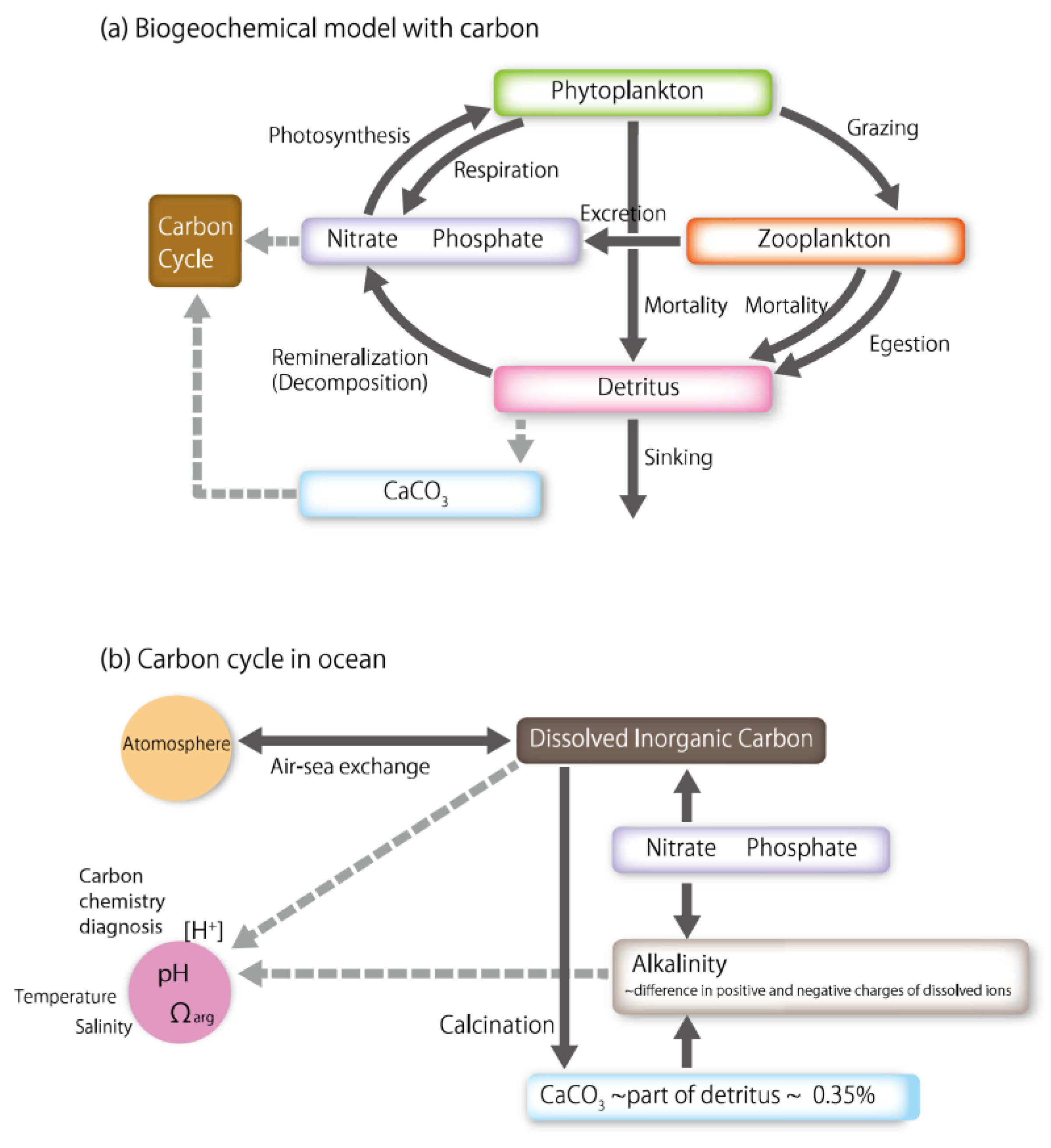
2.1. Equations Governing the Marine Ecosystem Model

A simple nitrogen-based plankton ecosystem model (NPZD) was used. It comprised five components including dissolved inorganic nitrogen (DIN, NO3), dissolved inorganic phosphate (DIP, PO4), phytoplankton (P), zooplankton (Z) and detritus (D) [26,27]. The carbon cycle model comprised three components: DIC, ALK and calcium carbonate (CaCO3), and was coupled with the NPZD model. Detritus corresponded to the concentrations of particulate organic nitrogen (PON). The pH (pHinsitu, pH25) and Ωarg values were calculated from temperature, salinity, DIC and ALK using a Fortran program based on the CO2sys MATLAB software [39,40]. The development of the nitrogen-based plankton ecosystem model followed the outlines described by Guo and Yanagi [27], Onitsuka and Yanagi [26] and Sasai et al. [25] (Figure 2a). The carbon cycle model is referred from Orr et al. [41], Ewen et al. [42] and Schmitnner et al. [18] (Figure 2b).
The source-sink terms for each individual biological tracer were defined by the following equations:
d P d t = P h t o s y n t h e s i s   ( D I N , D I P , P ) Re s p i r a t i o n   ( P ) M o r t a l i t y   ( P ) G r a z i n g   ( P , Z ) ,
d Z d t = G r a z i n g   ( P , Z ) M o r t a l i t y   ( Z ) E g e s t i o n   ( Z ) E x c e r t i o n   ( Z ) ,
d D d t = E g e s t i o n   ( Z ) + M o r t a l i t y   ( P ) + M o r t a l i t y   ( Z ) D e c o m p o s i t i o n   ( D ) z ( W D D ) ,
d ( D I N ) d t = P h t o s y n t h e s i s   ( D I N , D I P , P ) + R e s p i r a t i o n   ( P ) + E x c e r t i o n   ( Z ) + D e c o m p o s i t i o n   ( D ) Clim _ D a m p ( D I N )
d ( D I P ) d t = 1 R P : N d ( D I N ) d t Clim _ D a m p ( D I P ) ,
where W D is the sinking velocity of detritus, RP:N is the Redfield ratio of P (phosphorus):N (nitrogen) (Table 1). The biogeochemical processes represented in Equations (1)–(5) are as follows:
P h o t o s y n t h e s i s   ( D I N , D I P , P ) = V max exp ( C T P T ) × min ( D I N D I N + K D I N , D I P D I P + K D I P ) × I ( P ; z ) I o p t exp ( 1 I ( P ; z ) I o p t ) × P ,
where T is the seawater temperature, Vmax is the maximum growth rate from photosynthesis, and KDIN and KDIP are half saturation constants for DIN and DIP, respectively. We adopted optimal uptake kinetics for KDIN relating to Vmax, according to the theory of physiological acclimation of phytoplankton [25,43], defined as: K D I N = V max / A + 2 V max D I N / A ( μ mol l 1 ) and K D I P = V max / A + 2 V max R P : N D I P / A ( μ mol l 1 ) , where A is an affinity coefficient of basic cellular physiology representing the efficiency of nutrient encounters at the phytoplankton cell surface, RP:N is the stoichiometry of N to P [44,45], C T P is a temperature-dependent coefficient for photosynthesis, and Iopt is the optimum light intensity. I(P;z) is the light intensity at depth z, and is determined by solar radiation at the sea surface (Is) and the light extinction coefficient, ĸ(P). These relationships are given by
I ( P ; z ) = I s exp ( 0 z κ ( P ) d z ) ,
where ĸ(P) = cdom + 0.054 P0.6667 + 0.088 P, cdom is the light dissipation coefficient of seawater. ĸ(P) depends on cdom and a shelf shading effect influenced by phytoplankton [21,27].
The respiration (extracellular excretion) of phytoplankton, and the mortality of phytoplankton and zooplankton were defined as follows:
Respiration   ( P ) = R × exp ( C T R P T ) × P ,
Mortality ( P ) = M P × exp ( C T M P T ) × P 2 ,
Mortality ( Z ) = M Z × exp ( C T M Z T ) × Z 2 ,
where C T R P , C T M P , and C T M Z are temperature-dependent coefficients for the respiration of phytoplankton, and the mortality of phytoplankton and zooplankton, respectively. The respiration of phytoplankton was assumed to be proportional to its concentrations and rate of photosynthesis. The mortality rates for phytoplankton and zooplankton were assumed to be proportional to the square of their concentrations (biomass).
The grazing of phytoplankton by zooplankton was defined as a function of temperature and the concentrations of phytoplankton and zooplankton, expressed as
Grazing ( P , Z ) = G Z × max { 0 ,   1 exp ( λ ( P P ) ) } × exp ( C T G Z T ) × Z ,
where C T G Z is the temperature dependent-coefficient of grazing by zooplankton, Gz is the maximum rate of grazing of phytoplankton at 0 °C, P* is the threshold phytoplankton concentration for possible grazing by zooplankton, and λ is the Ivlev constant. Zooplankton were assumed to graze only on phytoplankton.
Excretion and egestion by zooplankton were assumed to be proportional to their grazing and predating, as defined by
Egestion   ( Z ) = ( 1 α Z ) × G r a z i n g ( Z ) ,
Excretion   ( Z ) = ( α Z β Z ) × G r a z i n g ( Z ) ,
where αz and βz are assimilation and growth efficiency constants for zooplankton, respectively.
The decomposition of detritus is dependent on the water temperature and was expressed as follows:
Decomposition   ( D ) = V D × exp   ( C T λ D T ) × D ,
where VD is the decomposition rate at 0 °C, and C T λ D is the temperature coefficient of decomposition.
Climatology damping conditions were adapted for the DIN and DIP source–sink terms, and were defined as follows:
Clim _ D a m p ( D I N ) = γ ( D I N D I N clim ) ,
Clim _ D a m p ( D I P ) = γ ( D I P D I P clim ) ,
where γ is the inverse of the time scale (= 30 days), and DINclim and DIPclim are the monthly climatology data for DIN and DIP, respectively. Some details of climatology damping are described in Section 3.1.

2.2. Equations Governing the Carbon Cycle Model

The modeling of the air–sea gas exchange and carbon chemistry followed the protocols from the Ocean Carbon-Cycle Model Intercomparison Project (OCMIP) [41,42]. Biological uptake and release occur in fixed elemental ratios for C, P and/or N. The production of DIC and ALK was controlled by changes in the inorganic nutrients (DIN, DIP) and calcium carbonate (CaCO3) in molar relationships as follows:
d ( D I C ) d t = d ( D I P ) d t R C : P d ( C a C O 3 ) d t Clim _ D a m p   ( D I C ) ,
d ( A L K ) d t = d ( D I N ) d t R A L K : N 2 d ( C a C O 3 ) d t Clim _ D a m p   ( A L K ) ,
where RC:P and RALK:N are the molar elemental ratios of C to P, and of ALK to N, respectively.
Climatology damping conditions were also adapted for the DIC and ALK source–sink terms, as follows:
Clim _ D a m p ( D I C ) = γ ( D I C D I C clim ) ,
Clim _ D a m p ( A L K ) = γ ( A L K A L K clim ) ,
where DICclim and ALKclim are monthly climatology data for DIC and ALK, respectively (see Section 3.1).
Calcium carbonate (CaCO3) immediately sinks after its production. We did not treat the CaCO3 concentration as a predictable variable in this model. The equations for approximating CaCO3 were as follows:
d ( C a C O 3 ) d t = Pr   ( C a C O 3 ) Pr   ( C a C O 3 ) d z d d z ( e z / D C a C O 3 ) ,
Pr   ( C a C O 3 ) = ( E g s e t i o n ( Z ) + M o r t a l i t y ( P ) + M o r t a l i t y ( Z ) ) R C a C O 3 / P O C R C : P ) ,
where DCaCO3 is the CaCO3 remineralization e-folding scale depth, and RCaCO3/POC is the ratio of CaCO3 to the non-photosynthetic production of particulate organic carbon (POC). Pr (CaCO3) is parameterized as a fixed ratio (RCaCO3/POC) of the production of non-diazotrophic detritus [18].

2.3. Inorganic Carbon Cycling in Water

The chemical reactions in water involve the carbon–water–borate system [47]. This system describes the relationships among [DIC], [ALK], [H+], and borate (BOR), whereby
[ A L K ] = ( 2 k 1 k 2 X 2 1 + k 1 X + k 1 k 2 X 2 ) [ D I C ] + ( k b 1 + k b X ) [ B O R ] + k w X X 1 ,
[ B O R ] = [ B ( O H ) 4 ] + [ H 3 B O 3 ] ( 0.00232 / 10.81 ) ( S / 1.80655 ) ,
where BOR can be approximated using a known parameter of salinity, S, and X = 1/[H+] (note that pH = −log10[H+]). These parameters were solved iteratively, as [ALK] approximates the carbonate alkalinity according to
[ A L K ] c = 2 [ C O 3 2 ] + [ H C O 3 ] = ( 2 k 1 k 2 X 2 1 + k 1 X + k 1 k 2 X 2 ) [ D I C ] .
As γc = [ALK]/[DIC], Equation (23) can be reduced to an iterative solution of the following two equations for two unknowns, X and γc [47,48]:
γ c = [ A L K ] [ D I C ] ( k b X k b + 1 ) [ B O R ] [ D I C ] [ k w X X 1 ] 1 [ D I C ] ,
X = ( γ c 1 ) k 1 + [ ( γ c 1 ) 2 k 1 2 + 4 γ c ( 2 γ c ) k 1 k 2 ] 1 / 2 2 ( 2 γ c ) k 1 k 2 .
γc is approximately 1.1, and this value can be used as a first guess. If X is known, the various ion concentrations can be defined [47] as follows:
[ C O 2 ] = [ D I C ] 1 + k 1 X + k 1 k 2 X 2 ,
P C O 2 = [ D I C ] / k 0 1 + k 1 X + k 1 k 2 X 2 ,
C O 3 2 = k 1 X 2 [ D I C ] 1 + k 1 X + k 1 k 2 X 2 ,
Ω arg = k 1 X 2 [ D I C ] 293.86 S k arg 1 + k 1 X + k 1 k 2 X 2 .
The apparent dissolution constants k0, k1, k2, kb, kw, and karg are empirical functions of ambient temperature and salinity (see Mucci [49], Feely et al. [3] and other sources, cosys.m as summarized by Zeebe and Wolf-Gladrow [50]). The algorithm was checked using typical representative values provided by Machkenzie et al. [51], except for Ωarg.
The ALK flux at the sea surface was set to zero, while the DIC flux in the form of CO2 gas was assumed to be proportional to the difference in the partial pressures of CO2 in surface waters (PCO2) and the atmosphere ( P C O 2 a t m ) [47,50], as described by
F D I C = ρ w V p k 0 C ( P C O 2 P C O 2 a t m ) ,
F A L K = 0 ,
where ρw is the seawater density, and k0c is the solubility of CO2 in seawater in mol kg−1 atm−1 [52,53,54], and is expressed as follows:
k 0 C = exp ( 9345.17 ( 1 T ) 60.2409 + 23.3585 log ( T 100 ) + S ( 0.023517 0.023659 ( T 100 ) + 0.0047036 ( T 100 ) 2 ) ) ,
where T is in units of Kelvin, and Vp is the piston velocity, which depends on wind speed U10 and the Schmidt number (Sc), and is expressed in units of m s−1 [53] as follows:
V p = 8.61 × 10 7 U 10 2 ( S c / 660 ) 1 / 2 .
Sc is a function of the ambient temperature T (in °C), and, for CO2, is expressed as follows:
S c = 2073.1 125.62   T + 3.627   T 2 0.043219   T 3 .

3. Data and Model Parameters

3.1. Climatology and Forcing Data

We created monthly DIN and DIP climatological data on the model grid by interpolating the original data from the World Ocean Atlas 2013 (WOA13). Yasunaka et al. [55] created a monthly climatology for surface DIN and DIP in the North Pacific (10°–60° N, 120° E–90° W). We replaced the surface values for DIN and DIP in the WOA13 with the data from Yasunaka’s study, in an area defined by 10.5°–60° N and 120°–180° E.
A climatological DIC database was created by combining an annual mean climatology product estimated using the method of Goyet et al. [56] with temperature and salinity data from the WOA climatology and the annual mean climatological datasets created by Key et al. [57]. There were no monthly climatology datasets available, except for the monthly surface climatology datasets of Yasunaka et al. [58]. We therefore replaced the surface values in the climatology database with Yasunaka’s climatology data, for an area defined by 10.5°–60° N and 120°–180° E.
There were no sophisticated climatological datasets for ALK for the study region [46,56,57,59]. Consequently, we first combined two climatology datasets estimated by Goyet et al. [27] with temperature and salinity data from the WOA13 climatology and the annual mean climatology of Key et al. [57], and then replaced the surface data for depths above 200 m with the data estimated using Takatani’s method [46].
We found that the first version of the created ALK data was significantly different from the ALK observed data obtained for the Japan Sea for the period 1997–2017, downloaded from the Japan Meteorological Agency (JMA) website, so we replaced the ALK data for the Japan Sea with the JMA observed data, on the assumption that the JMA data had the characteristics of ALK profiles in the Japan Sea.
After all the processes for creating the monthly climatological data for DIN, DIP, DIC and ALK were completed, we applied Gaussian smoothing with a spatial decorrelation scale (e-folding scale) of 100 km to remove any horizontal gaps in the data that may have formed during the repeated operations that combined the different data sources.
The model required forcing data to drive photosynthesis and CO2 gas exchange in the surface/subsurface layer. Short wave radiation ( I s ) was derived from the 6-hourly NCEP/NCAR (National Centers for Environmental Projection/National Center for Atmospheric Research) reanalysis data. Monthly mean values for the partial pressure of carbon dioxide ( P C O 2 a t m ) are available at the JMA website. Using data from the Ayasato Observatory in Japan, we created an empirical formula for CO2 (in ppm) with the addition of a second-order polynomial (CO2poly) and seasonal sinusoidal curve equations (CO2curv), as follows:
C O 2 p o l y = 0.000633 × t y r 2 0.650417 × t y r 859.0625 ,
C O 2 c u r v = 0.00064 + 6.09254 cos ( 2 π 24 × 365 t h r 55.20975 2 π 360 ) + 0.39431 cos ( 2 π 24 × 91.25 t h r 120.3614 2 π 360 ) ,
where tyr and thr are the Julian year and the time in hours from 1 January each year, respectively.
The left-hand terms in Equations (1)–(5), (17) and (18) denote transport–diffusion equations for tracers. The daily mean velocities, sea level, and turbulent diffusion coefficient from the JCOPE2M were included in the transport–diffusion equations. The daily mean temperature and salinity from the JCOPE2M were also used to evaluate the source–sink terms in Equations (1)–(5), (17), (18) and (21).

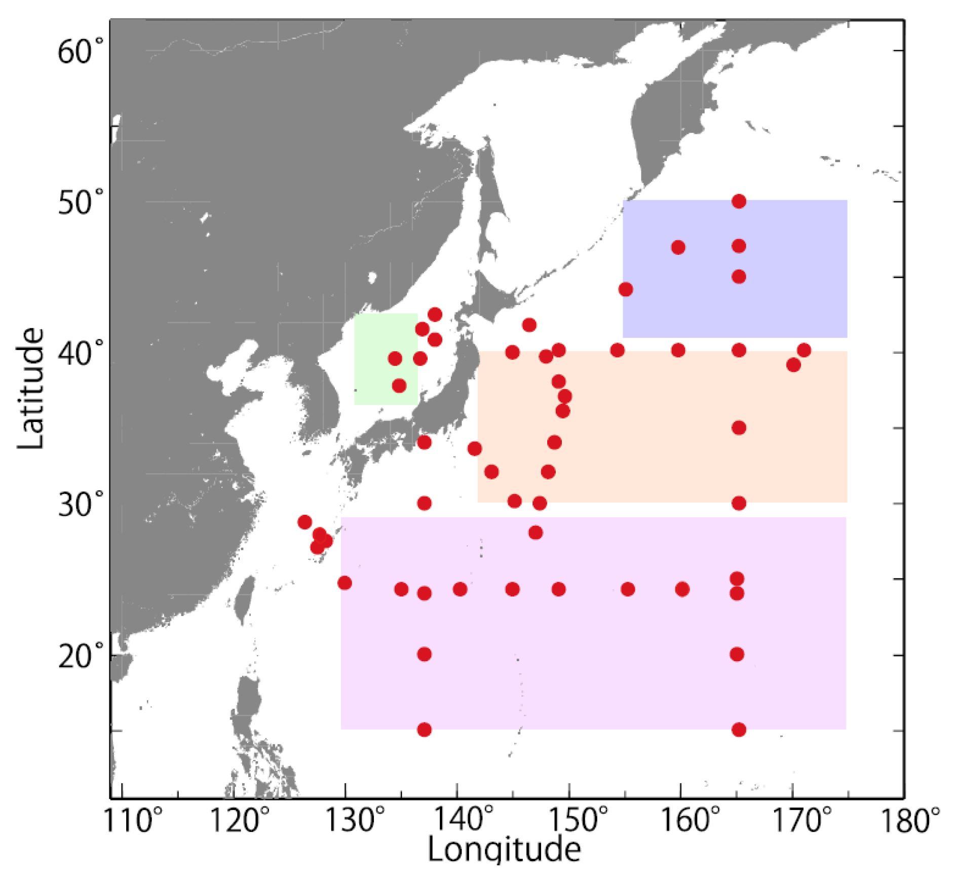
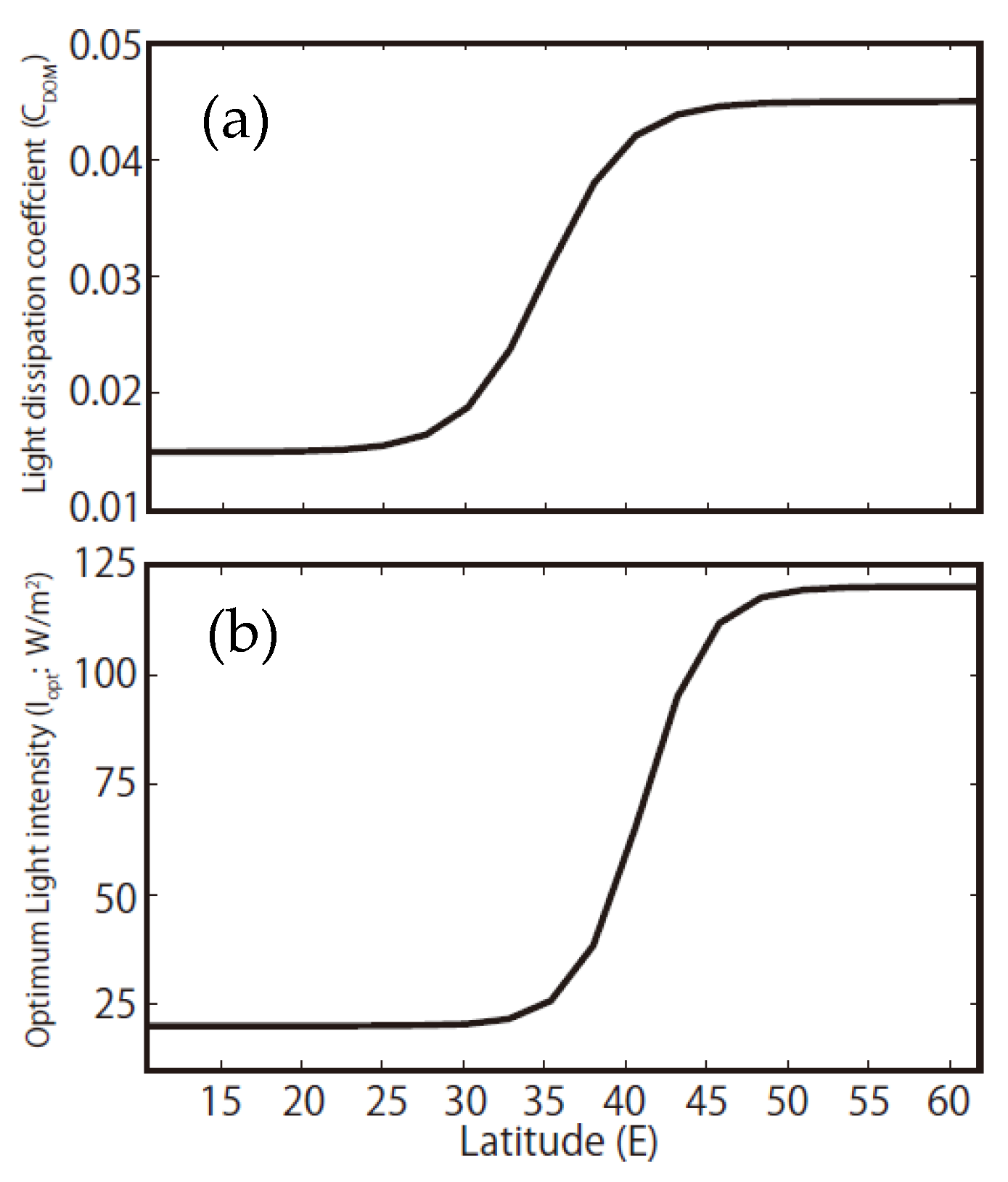
3.2. Biogeochemical Parameters and Observational Data for Validation

Table 1 shows the biogeochemical parameters used in our model, and the relevant reference values used by Onitsuka and Yanagi [26]. We adjusted the biogeochemical parameters by comparing the model outputs and the observed data in specific target regions (Figure 1, Table 2). The observed data were downloaded from the JMA website (Figure 1). The phytoplankton concentrations were also validated with chlorophyll-a data downloaded from an File Transfer Protocol (FTP) site for the Moderate Resolution Imaging Spectroradiometer (MODIS)-Aqua Ocean Color Data.
In previous studies, where biogeochemical models were applied to the North Pacific and the marginal seas of Japan, the target area was assumed to be occupied by the same type of water mass and/or the same water circulation gyres in the subarctic area [19,20,21,22,23,25], the subtropical area [21,25], and/or the marginal seas [27,60] (Figure 1). In contrast, our model included both subarctic and subtropical areas and adjoining marginal seas. As biogeochemical situations differ depending on oceanic conditions [61,62,63], in our model we applied latitudinal differences for Iopt and cdom, which were defined as follows:
I o p t = 0.5 I o p t 0 ( tanh ( ( L a t L a t b n d ) / L a t s l p ) + 1 ) + I o p t 1 ,
c d o m = 0.5 c d o m 0 ( tanh ( ( L a t L a t b n d ) / L a t s l p _ c d o m ) + 1 ) + c d o m 1 ,
where Iopt and cdom change latitudinally from 20 to 120 W/m−2 and from 0.015 to 0.045 m−1, respectively; I0opt, I1opt, c0dom, and c1dom are parameters for adjusting from subtropical to subarctic regions (Table 1 and Figure 3); and Latbnd and Latslp (Latslp_cdom) are the coefficients for latitudinal boundaries and the latitudinal slopes for these parameters, respectively (Table 1 and Figure 3). The effects of latitudinal differences on Iopt and cdom are described in Appendix A.
Using the Green’s function method [36], we optimized the biogeochemical parameters Vmax, R, Mp, Gz, Mz, VPN, and WD (Equations (6)–(16) and Table 1). Chlorophyll-a data for 2015 were used in these optimization operations, and we adopted the optimized operations for the subarctic and subtropical regions separately. All the estimated biogeochemical parameters were found to be similar to those for the subarctic and subtropical regions (Table 2), but we manually adjusted Vmax to 0.0492 day−1, after adopting the latitudinal differences for cdom and Iopt (Appendix A).

3.3. Initial and Boundary Conditions

We used a 1-year period, 2015, for all the experiments, which were driven by the forcing data for that year. In a preliminary experiment, the phytoplankton were represented by chlorophyll-a concentrations from the World Ocean Atlas 2001. There was undesirable noise in the model outputs for phytoplankton in the preliminary experiment, so, for the initial conditions, i.e., the beginning of the first month in the numerical experiments, constant values for phytoplankton of 0.05 and 0.0 μg/L were set for depths above 150 m and deeper depths, respectively, and the model was then run continuously. The initial zooplankton concentrations were set at 10% of the phytoplankton concentration. The initial detritus concentration was set at 0.0 mmol/kg.
As a first step towards developing reliable operational systems for biogeochemical parameters related to ocean acidification indices, we adopted a diagnostic approach to obtain realistic distributions for biogeochemical variables. The variables DIN, DIP and DIC were initialized using the climatology data for these parameters at the beginning of the 1-year simulation (January), and ALK was initialized using the annual climatology at the beginning. The climatology data for DIN, DIP, DIC and ALK were applied at all open lateral boundaries, and were included in the damping terms in Equations (15), (16), (19) and (20), with a 30-day time scale. The DIN, DIP and DIC climatology data used for the open lateral boundaries and the damping conditions (Equations (15), (16), (19) and (20)) were replaced by monthly data at the beginning of each month. Preliminary results showed that the damping condition was effective in representing smooth and realistic variations in the biogeochemical variables (not shown). Using this approach, we were able to predict biogeochemical variables over the short-term (within one month), driven by the forcing including the ocean and atmosphere reanalysis data with constraints on the climatology of DIN, DIP, DIC and ALK. All the experiments in this study were driven by the forcing created from the ocean (JCOPE2M) and atmospheric (NCEP/NCAR) reanalysis data.

4. Results

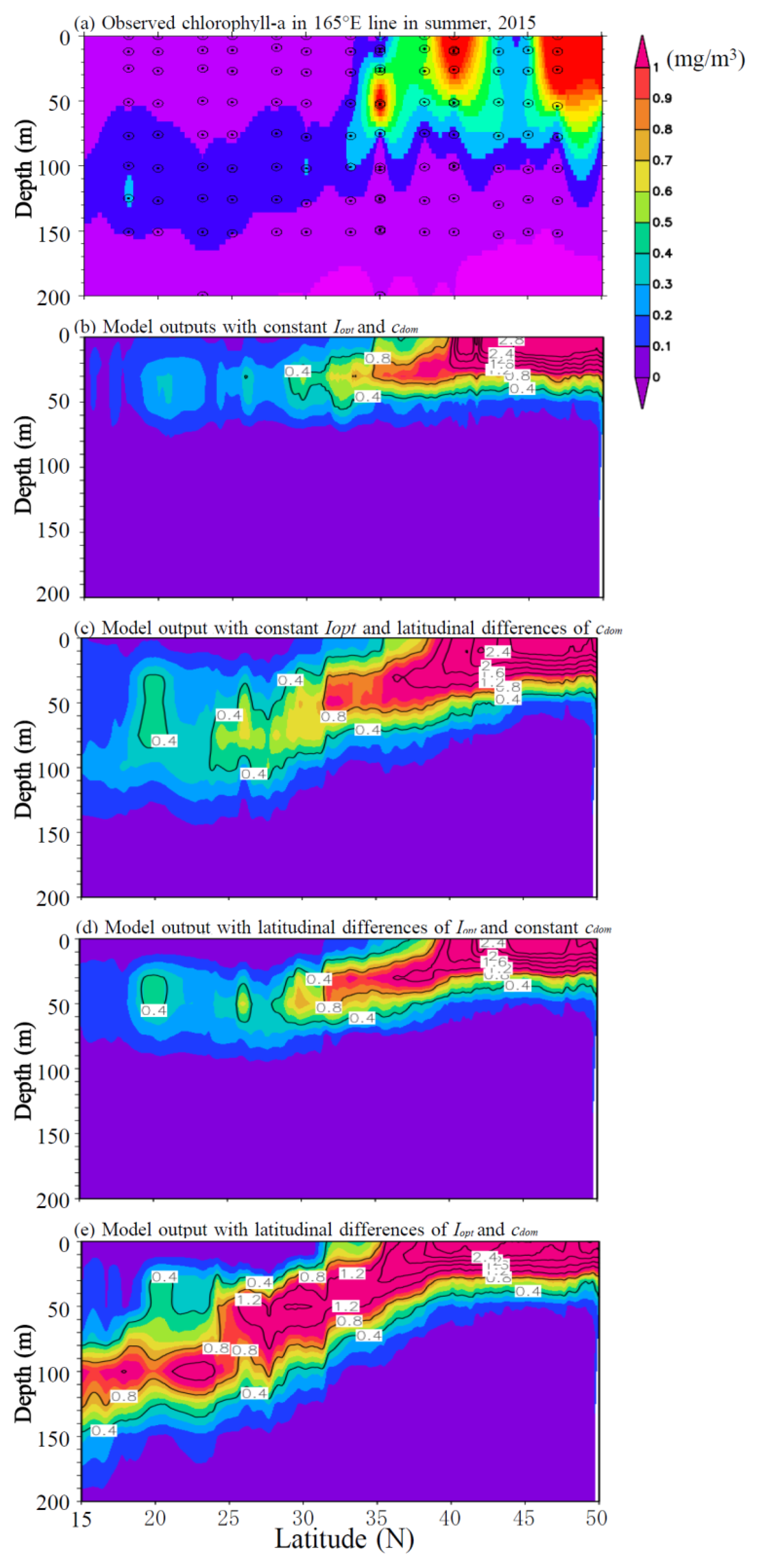
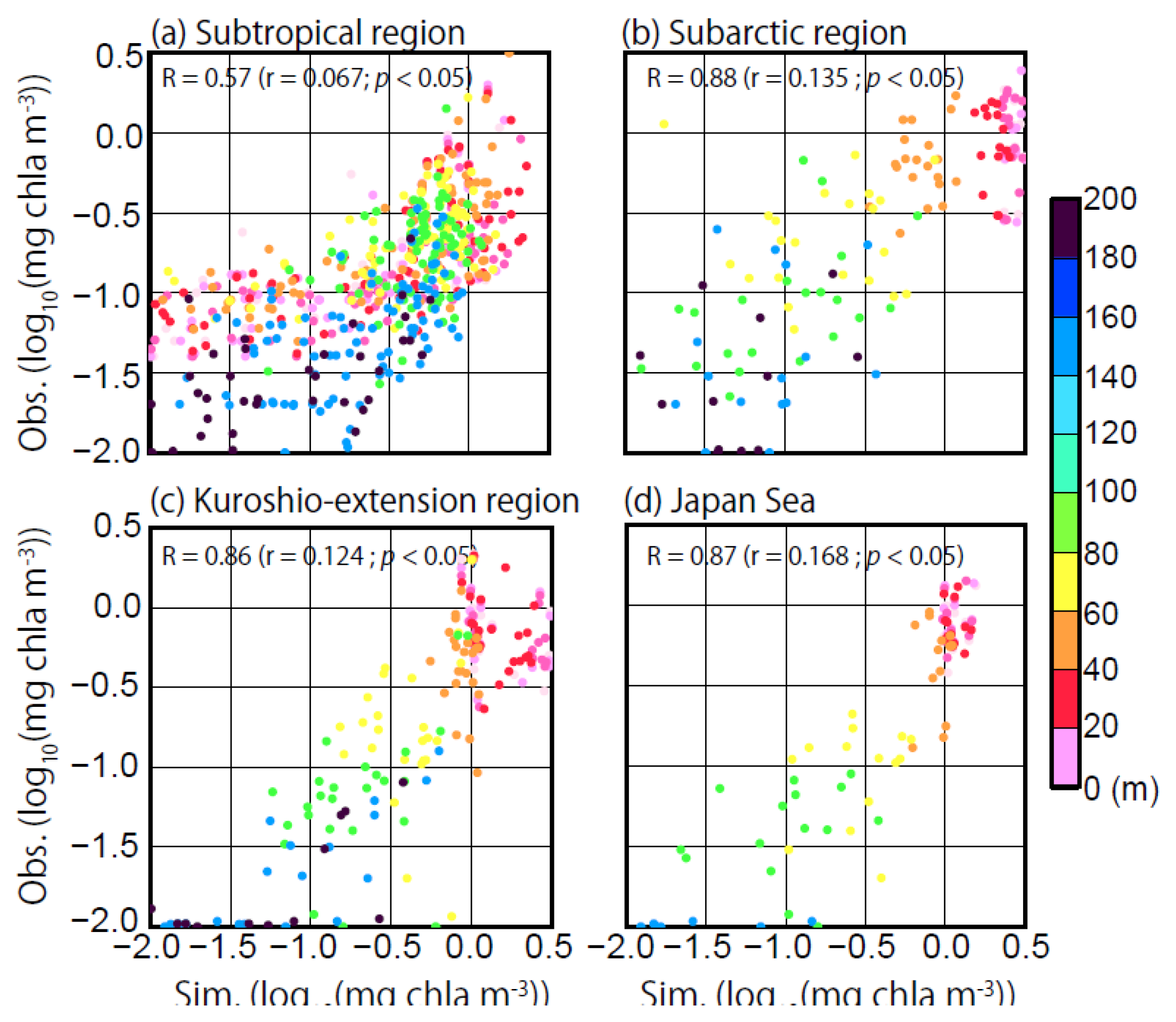
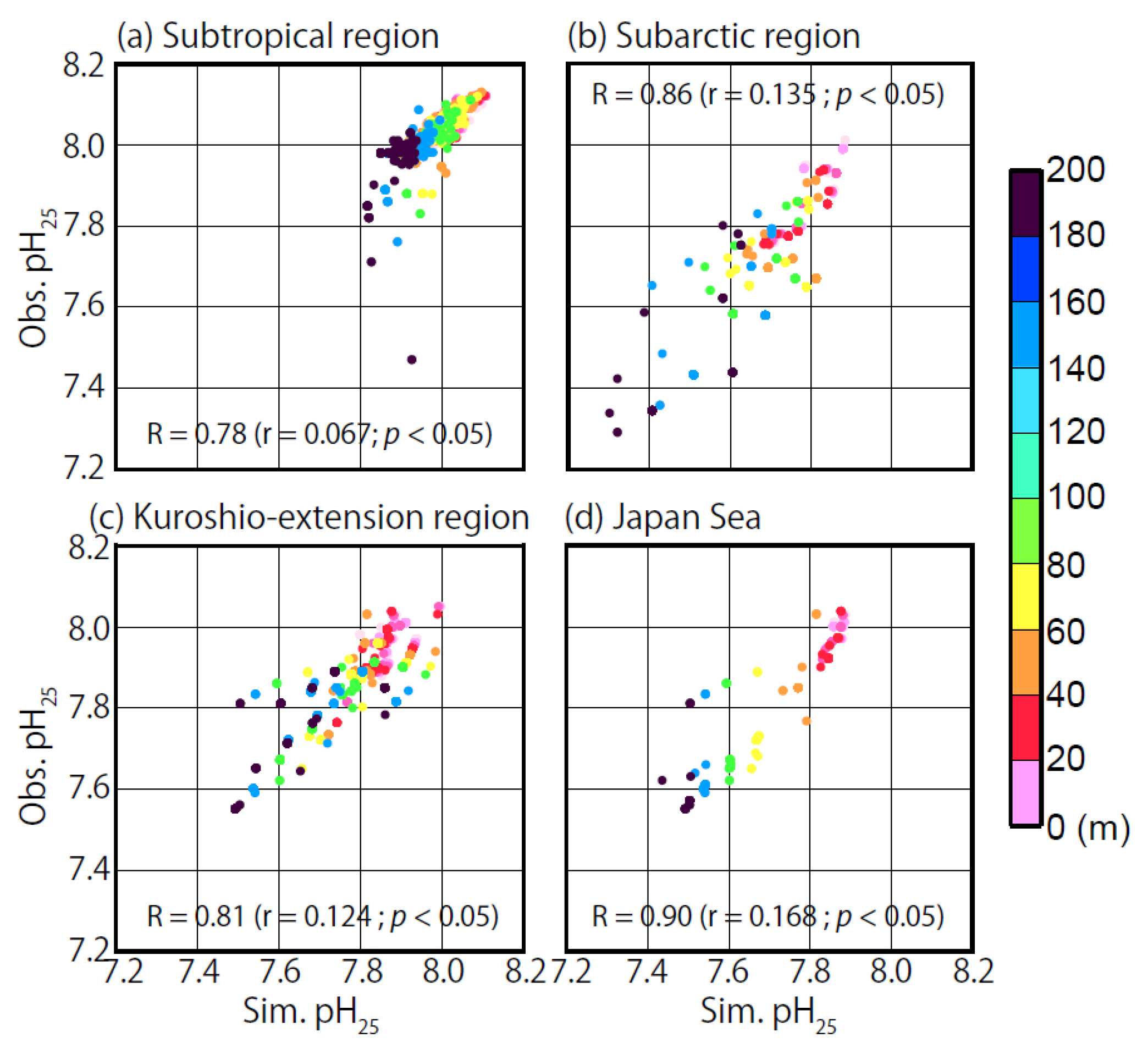
4.1. Comparison of the Observed Data with the Simulated Outputs

The monthly mean distributions of satellite and modeled chlorophyll-a values at the surface are shown in Figure 4. The satellite data show contrasting larger and smaller values in the subarctic and subtropical regions, respectively, throughout the year (Figure 4a–d and Figure 5a). The chlorophyll-a gradually increased to 2.0–3.0 milli mol/m3 at 50° N from March to May, and to 1.0–2.0 milli mol/m3 at 40° N, and remained high above 50° N during summer (June to July), with double peaks in spring and autumn around this latitude. There were also double peaks at 40° N in spring (March to May) and autumn (September to October) (Figure 5a). The model outputs basically reflected the observed chlorophyll-a distribution. The chlorophyll-a values were relatively large for areas above the region of 40° N, and were lower for areas at lower latitudes (Figure 4e–h). The model gave reasonable simulations of the chlorophyll-a variability, and the ranges were similar to the observed values (Figure 4e–h), but gave poor simulations of the seasonal patterns, particularly in the subarctic region (Figure 5a,b). The model reproduced only one notable peak in summer from May to August at 50° N (Figure 5b), and this peak lagged behind the observed data by 1–2 months (Figure 5a,b). Small and large double peaks were reproduced at 30° N and at 40° N, respectively. Consistent with the observed data (Figure 5a), the model reproduced small peaks for April and October at 20° N (Figure 5b).
The model gave adequate simulations of DIN and reproduced the basic features and seasonal variability, when the monthly climatology data were dampened (Figure 5c,d and Figure 6e–h). The climatology indicated large differences in the DIN concentrations between the subarctic and subtropical regions throughout the year (Figure 6a–d). The DIN values ranged from more than 4 μmol/kg above 45° N in the subarctic region to almost 0 μmol/kg in subtropical regions at various times of the year (Figure 6a–d). The modelled concentrations of DIN in the subtropical and subarctic regions were reasonably consistent with observed data. The seasonal variability in the climatology for the subarctic region above 40° N (Figure 5c and Figure 6a–d) was reproduced by the model (Figure 5d and Figure 6e–h). The modeled DIP distributions also reflected the observed data (not shown).
The concentrations of DIC (Figure 7a–d) were high (>2120 μmol/kg) in the Okhotsk Sea and the northwestern North Pacific along the Kamchatka Peninsula and the Kuril Islands in winter (January) and spring (April) (Figure 7a,b). The concentrations were less than 2040 μmol/kg in the Kuroshio Extension region and in the subtropical region below 35° N (Figure 7a–d). There was noticeable seasonal variation in the concentrations (Figure 7a–d). For the Okhotsk Sea and northwestern North Pacific area mentioned above, DIN was not detected in the summer (July) or autumn (October) (Figure 7a–d). The model simulations were similar (Figure 7e–h), with a minor difference in the continental area of the Okhotsk Sea in summer and autumn (Figure 7c,d,g,h). The model reproduced the observed temporal variability in the surface DIC values for the latitudes in subtropical and subarctic regions along longitude 165° E (Figure 5e,f). The time-series in simulated DIC for 40° N showed a relatively larger decrease in DIC in summer (from July to September; Figure 5f) compared with the observed data for 40° N (Figure 5e).
Due to a lack of observed data, we could not compare the seasonal variations in ALK [13,26,52,53]. Instead of using the ALK climatology, we plotted the JMA observed data (Figure 8a–c). These data showed that the ALK concentrations were relatively low (2200–2250 μmol/kg) in the subarctic region above 40° N and in the Okhotsk Sea, and were higher (2250–2300 μmol/kg) below 40° N from spring to autumn (Figure 8a–c). The model simulations of the patterns of ALK in the subarctic region above 45° N in winter, spring and autumn (Figure 8d–f), and in the subtropical region in summer (Figure 8f), were similar. However, unlike the observed data, there was a marked decrease (50 μmol/kg) for summer in the subarctic region and the Okhotsk Sea (Figure 8f). The low values in summer were followed by higher values in autumn (Figure 8g). The time series for ALK (Figure 5g) also showed a decrease in summer around 40° N and 50° N. The summer decrease arose from the modeled variations in CaCO3 (not shown), and indicates that the summer decrease in ALK may have been overestimated.

4.2. Ocean Acidification Indices pH and Ωarg

Figure 9 shows the surface pHinsitu (pH25) and Ωarg values calculated from the model outputs for temperature, salinity, DIC and ALK (Figure 9a–d). The pHinsitu ranged from 7.85 to 8.10 in the northwestern Pacific area (Figure 9a–d), except in winter and spring (January and April) for the East China Sea near the coast of China (Figure 9a,b). The values in the side of Pacific basically ranged from 8.00 to 8.05. The values were lower (7.85–7.90) in the Okhotsk Sea and the Japan Sea throughout the year, and on the Pacific Ocean side along the Kamchatka Peninsula and Kuril Islands from winter to spring (Figure 9a,b). In the Kuroshio Extension region (140°–180° E, 30° N), the pH values were low during July (summer). The values were highest (8.10–8.15) in winter (January) and spring (April) (Figure 9a) between the subtropical and subarctic regions in the area corresponding to the Kuroshio extension. The values varied with latitude along the 165° E line (Figure 10a). The highest and lowest values occurred in February or March and June or August, respectively, in lower latitude regions around 20° N and 30° N, but the opposite occurred at around 40° N and 50° N (Figure 10a).
The pH25 values were lower in the northern region and higher in the southern region (Figure 9e–h). The lowest values (7.5–7.6) occurred in the Okhotsk Sea and along the Kamchatka Peninsula on the Pacific Ocean side in winter (January) and spring (April) (Figure 9e,f). The highest values (8.10–8.15) were found in the subtropical region at latitudes below 20° N. The pH25 values increased in summer (Figure 9e–h, Figure 10b). The amplitudes were larger in the northern region than in the southern region. The lowest and highest values at each latitude occurred in April and August, respectively.
The surface Ωarg values (>3.5) were high in the subtropical region, and low (2.0–3.0) in the subarctic region (Figure 9i–l). The values were lowest (1.0–1.5) in the Okhotsk Sea and along the Kamchatka Peninsula and the Kuril Islands on the Pacific Ocean side in winter (January) and spring (April). The values increased in summer (July), with similar spatial variability in autumn (October). The time-series at longitude 165° E showed that the Ωarg values were highest in August–September and lowest in April (Figure 10c), and the seasonal variation was similar to that for pH25 (Figure 10b).
Takahashi et al. [59] and Jiang et al. [64] created a global map of the surface climatology for pHinsitu and Ωarg in spring/summer and autumn/winter, but not for the Okhotsk, Japan and East China Seas. Their climatology showed that the pHinsitu and the Ωarg varied seasonally from 0.06 to 0.08 and from 0.50 to 1.00, respectively, in the subtropical, Kuroshio Extension, and were similar to the modeled values (Figure 9a–d,i–l). Yara et al. [65] studied the Ωarg distributions in a marginal area around Japan (24°–48° N, 118°–157° E). Their isothermal contours (Ωarg = 2.3 and 3.0), which reproduced the conditions in the 2010s (their Figure 7b), were similar to our model outputs (Figure 9i–l).

4.3. Reproducibility of the Biogeochemical Variables

The correlation coefficients between the JMA observed data and the model outputs for each region for 2015 were calculated for chlorophyll-a, DIN, DIC, pH25 and ALK (Table 3). The observed data and model outputs could be compared as they overlapped in time and location. The natural logarithm values of chlorophyll-a were calculated, as the plankton concentrations were not normally distributed but followed a lognormal distribution [66].
The correlation values were 0.57, 0.88, 0.86 and 0.87 for chlorophyll-a; 0.72, 0.88, 0.87 and 0.95 for DIN; 0.74, 0.87, 0.78 and 0.92 for DIC; 0.48, 0.69, 0.48 and 0.35 for ALK; 0.74, 0.86, 0.81 and 0.90 for pH25; and 0.99, 0.98, 0.98 and 0.99 for Ωarg, in the subtropical region, the subarctic region, the Kuroshio Extension and the Japan Sea, respectively (Table 2). Scatter plots (Figure 11, Figure 12 and Figure 13) showed that the parameters were highly correlated with each other (not shown for DIP, DIC and ALK).

5. Discussion

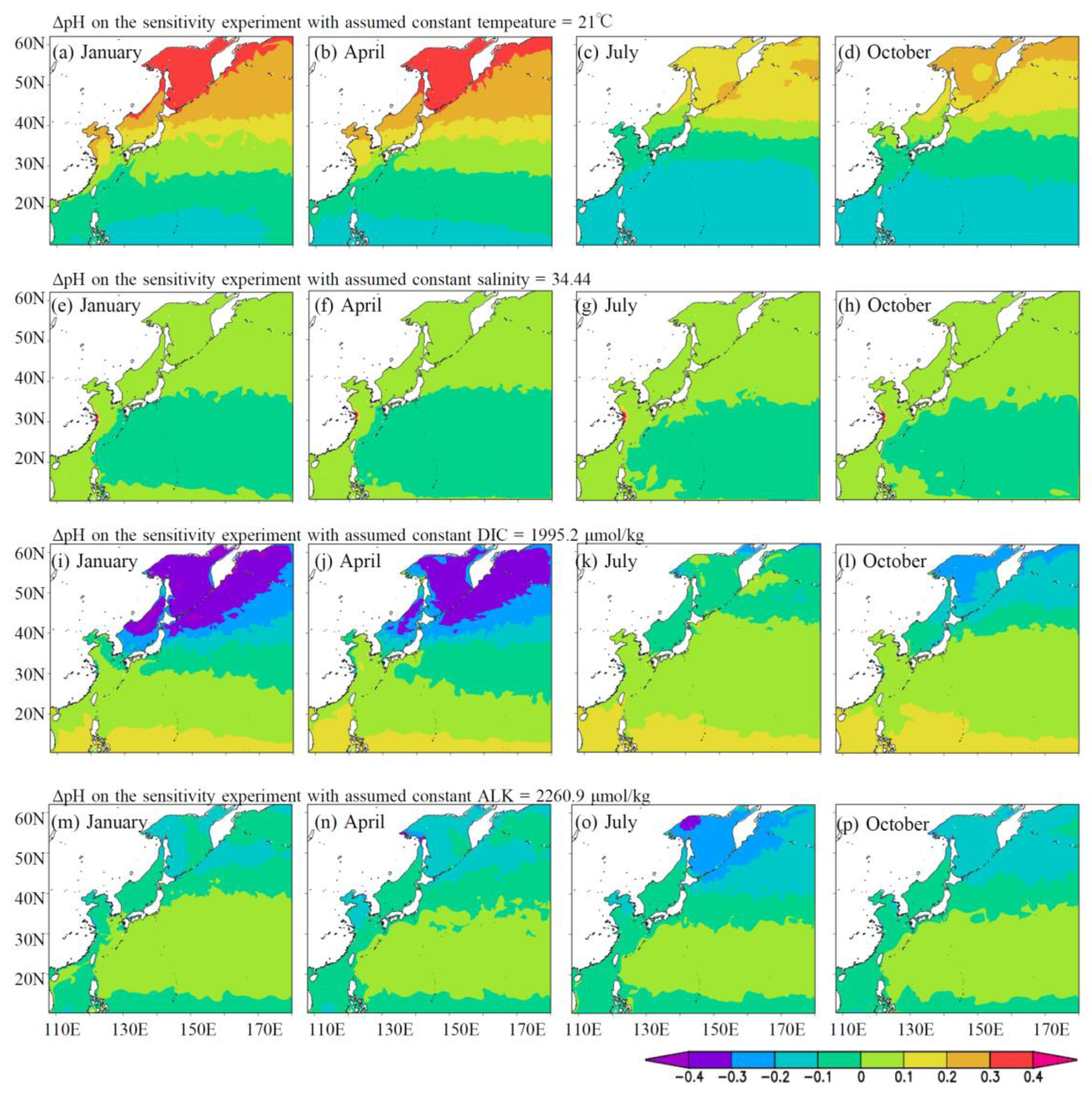
5.1. Sensitivity Experiment for pH and Ωarg Based on Constant Temperature, Salinity, DIC and ALK

To assess which variables were important in determining the ocean acidification indices pH and Ωarg, we performed a series of sensitivity experiments assuming a constant set of conditions for temperature (= 21 °C), salinity (= 34.44), DIC (= 1995.2 μmol/kg) and ALK (= 2260.9 μmol/kg). In the sensitivity experiments, pH and Ωarg were calculated with the assumed fixed variables of temperature, salinity, DIC and ALK, individually, in place of these original target variables of the model outputs. The other variables, except the assumed constant variables, were the same as those of the model outputs (Figure 4e–h, Figure 6e–h, Figure 7e–h and Figure 8; Section 4). The assumed constant variables were determined by the values corresponding to median values calculated from the model outputs in the region of 10.5°–62° N and 108°–180° E in the surface in January (e.g., Figure 6e and Figure 7e).
Figure 14 shows the horizontal distributions of the surface pH difference (ΔpH), which was calculated by subtracting the model output for each sensitivity experiment using each fixed temperature, salinity, DIC and ALK value from the basic model outputs shown in Figure 9a–d. Measuring the differences enabled the individual effects of each target variable to be assessed. The temperature and DIC had most influence on the pHinsitu in winter, spring and autumn, while ALK had a considerable influence in summer.
The variables that had most influence on Ωarg throughout the year were DIC and ALK (Figure 15). The sensitivity experiments using the fixed values for temperature, DIC and ALK (Figure 15) showed positive effects in the subarctic region and negative effects in the subtropical region. The effects of temperature and salinity, while detectable, were small compared with the effects of DIC and ALK (Figure 15e–h).

5.2. Effect of Seasonal Processes on pHinsitu

The sensitivity analysis of the effect of temperature on pH showed a clear positive and negative contrast between the northern and southern regions, respectively (Figure 14a–d). This was related to the dissociation equilibrium: H2O↔H++OH. A relatively low (high) temperature in the northern (southern) region resulted in an increase (decrease) in the pH by shifting the equilibrium in the direction: H2O←H++OH (H2O→H++OH). With the transition from winter to summer, the pH decreased throughout the entire region as a result of increasing temperature (Figure 14a–c), while the pH increased with cooling in autumn in some parts of the northern region (Figure 14d).
The horizontal distribution of surface DIC (Figure 7e–h) led to a significant negative and positive contrast between the northern and southern regions, respectively (Figure 14i–l). This was associated with the CO2 equilibrium in sea water, defined by: CO2+H2O↔H++HCO3. Relatively high (low) DIC concentrations in the northern (southern) region tended to result in lower (higher) pH values by shifting the equilibrium in the direction: CO2+H2O→H++HCO3 (CO2+H2O←H++HCO3). The decrease in DIC from winter to summer (Figure 7e–g) caused the pH to increase throughout the entire region (Figure 14j,k), by shifting the equilibrium in the direction: CO2+H2O←H++HCO3.
The relatively high concentration of ALK in the subtropical gyre (Figure 8a–d) resulted in a relatively high pH (Figure 14m–p). As the ALK decreased from winter to summer (Figure 8a–c) the pH decreased throughout the entire region (Figure 14m–o). This trend was more evident in the northern region than in the southern region (Figure 14o), reflecting the relatively enhanced decrease in ALK in the northern region (Figure 8c).
The sensitivity of salinity to pH was not significant compared with the other variables, and the seasonal variability in pH caused by the variation in salinity was also minor (Figure 14e–h). Lower salinity levels led to higher pH values, and was locally evident around the mouth of the Changjiang River.
From the sensitivity analyses, we inferred that overall seasonal variations in the pHinsitu (Figure 9a–d and Figure 10a) were largely governed by the balance between temperature and DIC, and to a lesser extent by ALK. In the southern region, the relationship with temperature was relatively important, and thus the pHinsitu decreased from winter to summer. In contrast, the pHinsitu increased slightly from winter to summer in the northern region, where the relationship with DIC and ALK was slightly stronger. The pH25 variation mainly reflected the effects of DIC and ALK variations (Figure 9e–h and Figure 10b). However, the model probably overestimated a decrease in ALK in summer, as shown in Figure 8b,f, and the variations in the pHinsitu may actually be mainly governed by temperature and DIC.

5.3. Seasonal Processes Affecting Ωarg Variations

The sensitivity of the target variables to Ωarg are shown in Figure 15. The temperature dependence of Ωarg can be explained by the characteristics of the aragonite solubility product, kargarg = ([Ca2+][CO32−])/karg). The value of karg decreases as the water temperature increases [34]. Latitudinal differences in the sensitivity of temperature resulted in higher and lower Ωarg values in the southern and northern regions (Figure 15a–d), respectively. Seasonal warming/cooling affected the seasonal variation in Ωarg throughout the entire region.
The reaction for the dissolution of marine carbonate [3,6], CO2+H2O+CO3↔2HCO3, was related to latitudinal differences in the sensitivity of DIC (Figure 15i–l). As the DIC concentration was relatively high in the northern region (Figure 7e–h), the concentration of carbonate ions (CO3) was relatively low, and consequently the Ωarg value was relatively low in this region (Figure 15i–l). The seasonal decrease in DIC from winter to summer caused the Ωarg values to increase throughout the entire region (Figure 15k). The sensitivity of ALK to Ωarg showed that higher ALK levels led to higher Ωarg values because the higher ALK levels were related to higher carbonate ion concentrations. With a decrease in ALK in the northern region from winter to summer (Figure 8a–c), the Ωarg values tended to decrease (Figure 15m–o). The sensitivity of salinity to Ωarg (Figure 15e–h) was low, and similar to that of the pHinsitu (Figure 14e–h).
From the sensitivity analysis, we inferred that DIC and ALK had most impact on the seasonal variability in Ωarg across the entire region throughout the year, with less of a temperature effect. However, the summer increase in Ωarg (Figure 10c) was mainly the result of the decrease in DIC in summer (Figure 9i–l and Figure 10c), because the model probably overestimated a decrease in ALK in summer and the decrease in ALK and the increase in temperature in summer together caused a decrease in Ωarg.

6. Conclusions

We developed a new biogeochemical model (JCOPE_EC) for carbon processes, based on the physical background of a numerical model product, JCOPE2M, which is a three-dimensional operational eddy-resolving model product. Comparison with observed data for 2015 showed that the JCOPE_EC model adequately reproduced the basic features of chlorophyll-a, DIN (DIP), DIC and ALK. The seasonal variability in these biogeochemical variables was similar to the observed (climatological) variability, although the modelled seasonal variability in chlorophyll-a and ALK deviated somewhat from the observed.
The overestimation of the increase in chlorophyll-a in the subarctic region (Figure 4 and Figure 5b) may be related to iron cycling, which was not included in JCOPE_EC [67]. Iron cycling may also explain the overestimates of biological production of CaCO3 and also ALK reduction (Figure 5g and Figure 8f). The present model will need to be improved to account for these processes.
The JCOPE_EC also represented the ocean acidification indices pH and Ωarg, based on the model outputs for temperature, salinity, DIC and ALK. The simulated values were consistent with observed data, although the pHinsitu and Ωarg values in some parts in the Okhotsk Sea and the Japan Sea from winter to spring were lower than expected (Figure 9a–d,i–l). This is probably a consequence of the uncertainty in the climatology data for these parameters, and should be investigated more fully.
Sensitivity experiments, aimed at assessing which variables had most effect on the ocean acidification indices, were performed using fixed values for temperature, salinity, DIC and ALK. The results showed that seasonal variations in pHinsitu were largely governed by the corresponding balances between temperature and DIC, although ALK had some influence in summer in model. DIC was the main driver of the increases in the Ωarg from winter to summer, with some lesser effects of ALK and temperature. Salinity had little effect on pH and Ωarg, except around the Changjiang River mouth.
At present, it is difficult to operationally acquire nowcast/forecast information on biogeochemical variables at the basin scale. However, the JCOPE_EC was designed to use operational physical data from the JCOPE2M. Thus, with further improvements in its design, the JCOPE_EC could become an effective tool for providing realistic information about biogeochemical variables in the studied marine area.
The daily snapshots of the distributions of chlorophyll-a, DIN, pH, DIC and ALK in spring 2015 in Figure 16 and Figure 17 show that the JCOPE_EC was able to represent the distribution of biogeochemical factors associated with the meandering of the Kuroshio Current and other eddy phenomena. The Kuroshio Current transports water that is low in nutrients, DIC and ALK to downstream regions. Prominent areas of enhanced chlorophyll-a concentrations were evident, and their occurrence depended on ocean currents and the distribution of nutrient-rich waters (Figure 16). These mesoscale phenomena involve complex factors affecting DIC and ALK, and so affect the associated pH and Ωarg (Figure 17). Therefore, the JCOPE_EC has the potential to provide current realistic information on ocean acidification indices, which vary in space and time because of various oceanic phenomena, although validation and improvements in the model will be necessary.
By using this operational model (JCOPE_EC), we have already launched a trial to perform a nowcast/forecast experiment targeting ocean acidification indices (pHinsitu and Ωarg), which are reproduced with the nowcast/forecast operational ocean model products [35,36,38]. A website (https://www.marinecrisiswatch.jp/mcwatch/prediction/jcope/index.html) experimentally shows up-to-date results of the nowcast/forecast system to demonstrate our studies effectively.
The current version of the JCOPE_EC system includes climatology damping conditions for some biogeochemical variables, which highlights that the present model is diagnostic. To investigate the mechanisms that drive the modeled ecosystem and the carbon cycle, we will develop a more prognostic model without climatology damping in future studies, based on the present model. We also note that there is an extreme lack of publicly available observed biogeochemical data for the Okhotsk Sea and the East China Sea. We hope that the availability of observed data will improve, as, with more data, we can reduce the uncertainty in future model outputs for these regions.

Author Contributions

Conceptualization, T.T. and Y.M.; Methodology, Y.M. and M.I; Validation, M.I.; Formal analysis, M.I.; Writing—Original Draft Preparation, M.I.; Writing—Review and Editing, M.I. and Y.M.; Visualization, M.I.; Supervision, Y.M. and X.G.; Project administration, T.T.; Funding Acquisition, T.T. and. Y.M.

Funding

This research was funded by the Sasakawa Peace Foundation of the Ocean Policy Research Institute (OPRI-SPF).

Acknowledgments

We acknowledge the consistent support from the Sasakawa Peace Foundation of the Ocean Policy Research Institute (OPRI-SPF). This study is part of the Japan Coastal Ocean Predictability Experiment (JCOPE) promoted by the Japan Agency for Marine-Earth Science and Technology (JAMSTEC). NCEP/NCAR reanalysis data were downloaded from the websites of National Centers for Atmospheric Research: https://climatedataguide.ucar.edu/climate-data/ncep-ncar-r1-overview. World Ocean Atlas 2001 (WOA01) and 2013 (WOA13) data were downloaded from websites of the US National Oceanographic Data Center (NODC): https://www.nodc.noaa.gov/OC5/WOA01/pr_woa01.html and https://www.nodc.noa.gov/OC5/woa13/, respectively. Monthly climatology data for DIN, DIP, and DIC from Yasunaka et al. [24,60] were downloaded from: http://soop.jp/index.html. In-situ observed data obtained from the Japan Meteorological Agency (JMA) were downloaded from https://www.data.jma.go.jp/kaiyou/db/vessel_obs/data-report/html/ship/ship.php. Partial pressure data for carbon dioxide obtained at the Ayasato observatory were downloaded from https://ds.data.jma.go.jp/ghg/kanshi/obs/co2_monthave_ryo.html. Moderate Resolution Imaging Spectroradiometer (MODIS) Aqua Ocean Color data for 2015 were downloaded from the Physical Oceanography Distributed Active Archive Center (PODAAC) at ftp://podaac-ftp.jpl.nasa.gov/allData/modis/L3/aqua/4um/v2014.0/4km/daily/2015/.

Conflicts of Interest

The authors declare no conflict of interest.

Appendix A

Preliminary results showed that the chlorophyll-a maximum depth (Figure A1b) reproduced using constant coefficients for cdom and Iopt were shallower than the observed depths (Figure A1a). The chlorophyll-a reached a maximum at 0–50 m deep in the subarctic region of the northwestern Pacific, and this gradually deepened with distance southwards, and reached a maximum at 100–150 m deep in the subtropical region in summer (Figure A1a). The depths estimated by the preliminary model at which chlorophyll-a reached a maximum in the subtropical region (10°–20° N) were much shallower (above 50 m) for all latitudes (Figure A1b).
To reduce the bias in the preliminary model results for the chlorophyll-a maximum depth, we adopted values for cdom and Iopt that varied by latitude (Equations (39) and (40)) (Figure 3a,b). Using this approach, the model reproduced the vertical distribution and maximum depth of chlorophyll-a very effectively for the subtropical region, although the chlorophyll-a values (Figure A1c–e) were higher than the observation values (Figure A1a,e). As the parameter dependences of cdom and Iopt were nonlinear, we manually adjusted the parameter values after comparing the modeled and observational results.
Previous NPZD models of the marginal seas of Japan have used various constant Iopt values. For example, Kawamiya et al. [19,20,21] used an Iopt value of 48.8 W/m2 for station Papa (50.1° N, 144.9° W) [19,20] and the North Pacific [21], Yamanaka et al. [48] used an Iopt value of 104.7 W/m2 for the North Western Pacific, Sasai et al. [25] used an Iopt value of 100 W/m2 for stations S1 and K2, Kishi et al. [22] used an Iopt value of 104.7 W/m2 for the subarctic region of the North Pacific, Guo and Yanagi et al. [27] used an Iopt value of 150.0 W/m2 for the East China Sea, and Onitsuka and Yanagi [26] used an Iopt value of 70.0 W/m2.
Edwards et al. [61] characterized growth-irradiance relationships from information about 308 growth-irradiance experiments performed on 119 species of marine phytoplankton sampled from all major functional groups, and reported that the Iopt values did not vary among taxonomic groups. However, all traits varied considerably within most groups, and optic-ocean isolates tended to have lower Iopt values than coastal isolates. This implies that phytoplankton may change their physiological characteristics depending on the light environment. Their study appears to be consistent with the latitudinal difference we found for Iopt.
Various studies have used constant values ranging from 0.035 to 0.04 m−1 for cdom in the North Pacific [19,20,21,22,25,48]. These cdom values represent light dissipation coefficients, which are linked to the distribution of chromophoric dissolved organic matter. Nelson and Sigel [63] showed that the absorption of surface chromophoric dissolved organic matter plus detrital particle at 443 nm was 0.005 m−1 in the subtropical region of the North Pacific but gradually increased to 0.05 m−1 in the subarctic region. This indicates that the distribution of chromophoric dissolved organic matter make more invisible the subsurface layer in the subarctic region than in the subtropical region. The latitudinal difference for cdom used in the present study represents a change from 0.015 m−1 in the subtropical region to 0.045 m−1 in the subarctic region (Figure 3a), which is consistent with observed distributions of chromophoric dissolved organic matter [63].
Figure A1. Vertical distribution of chlorophyll-a (mg/m3) along longitude 165° E from JMA observations in 2015 (a) and model outputs (be). The figure shows the sensitivity experiment results with (b) constant Iopt (= 70 W/m2) and cdom (= 0.04 m−1); (c) constant Iopt (= 70 W/m2) and latitudinal differences for cdom; (d) latitudinal differences for Iopt and constant cdom (= 0.04 m−1); and (e) latitudinal differences for Iopt and cdom (the results of the model outputs as shown in Figure 4e–h).
Sustainability 11 02677 g0a1

References

  1. Baur, J.F.; Cai, W.J.; Raymond, P.A.; Bianchi, T.S.; Hopkinson, C.H.; Pierre, A.; Regnier, P. The changing carbon cycle of the coastal ocean. Nature 2013, 504, 61–70. [Google Scholar] [CrossRef]
  2. Bednarsek, N.; Feely, A.R.; Reum, J.C.P.; Peterson, B.; Menkel, J.; Alin, R.S.; Hales, B. Limacina helicina shell disoolution as an indicator of declining habitat suitability owing to ocean acidification in the California Current Ecosystem. Proc. Biol. Sci. 2014, 281, 20140123. [Google Scholar] [CrossRef] [PubMed]
  3. Feely, A.R.; Sabine, L.C.; Barne, H.R.; Millero, J.F.; Dickson, G.A.; Wanninkhof, R.; Murata, A.; Miller, A.L.; Greeley, D. Decadal changes in the aragonite and calcite saturation state of the Pacific Ocean. Glob. Biogeochem. Cycles 2012, 26, GB3001. [Google Scholar] [CrossRef]
  4. Stocker, T.F.; Qin, D.; Plattner, G.-K.; Tignor, M.M.B.; Allen, S.K.; Boschung, J.; Nauels, A.; Zia, Y.B.; Midgley, P.M. (Eds.) Intergovernmental Panel on Climate Change (IPCC), Climate Change 2013: The Physical Science Basis. In Contribution of Working Group I to the Fifth Assessment Report of the Intergovernmental Panel on Climate Change; Cambridge University Press: Cambridge, UK; New York, NY, USA, 2013; pp. 1–1535. [Google Scholar]
  5. Kroeker, J.K.; Kordas, L.R.; Crim, R.; Hendrik, E.I.; Ramajo, L.; Singh, S.G.; Duarte, M.C.; Gattuso, P.J. Impacts of ocean acidification on marine organisms: Qualitifying sensitivities and interaction with warming. Chang. Biol. 2013, 19, 1884–1896. [Google Scholar] [CrossRef] [PubMed]
  6. Feely, A.R.; Alin, R.S.; Carter, B.; Bednarsek, N.; Hales, B.; Chan, F.; Hill, M.T.; Gaylord, B.; Sanford, E.; Byrne, H.R.; et al. Chemical and biological impacts of ocean acidification along the west coast of North America. Estuar. Coast. Shelf Sci. 2016, 183, 260–270. [Google Scholar] [CrossRef]
  7. Wittmann, C.A.; Portner, H. Sensitivities of extant animal taxa to ocean acidification. Nat. Clim. Chang. 2013, 3, 995–1001. [Google Scholar] [CrossRef]
  8. IGBP; IOC; SCOR. Ocean Acidification Summary for Policymakers. In Proceedings of the Third symposium on the Ocean in a High-CO2 World International Geoshpere-Bioshere Programme, Stockholm, Sweden, 14 November 2013. [Google Scholar]
  9. Bender, M.; Doney, S.; Feely, R.A.; Fung, I.; Gruber, N.; Harrison, D.E.; Keeling, R.; Moore, J.K.; Sarmiento, J.; Sarachik, E.; et al. A Large–Scale CO2 Observation Plan: In Situ Oceans and Atmosphere (LSCOP); NOAA OAR Special Report; National Oceanic and Atmospheric Administration: Silver Spring, MD, USA, 2002; pp. 1–201.
  10. Johnson, S.K.; Plant, N.J.; Coletti, J.L.; Jannasch, W.W.; Sakamoto, M.C.; Rise, C.S.; Swift, D.D.; Williams, L.N.; Boss, E.; Haentjens, N.; et al. Biogeochemical sensor performance in the SOCCOM profiling float array. J. Geophys. Res. Ocean 2017, 122, 6416–6436. [Google Scholar] [CrossRef]
  11. Doney, S.C.; Lima, I.; Feely, R.A.; Glover, D.M.; Lindsay, K.; Mahowald, N.; Moore, J.K.; Wanninkhof, R. Mechanisms governing interannual variability in upper-ocean inorganic carbon system and air-sea CO2 fluxes: Physical climate and atmosphere dust. Deep-Sea Res. II 2009, 56, 640–655. [Google Scholar] [CrossRef]
  12. Metz, N.; Tilbrook, B.; Bakker, D.; Quere, L.; Doney, C.; Feely, R.; Hood, M.; Dargaville, R. Global changes in ocean carbon: Variability and vulnerability. EOS Trans. 2007, 88, 287. [Google Scholar]
  13. Le Quere, C.; Orr, J.C.; Monfray, P.; Aumont, O. Interannual variability of the oceanic sink of CO2 from 1979 through 1997. Glob. Biogeochem. Cycles 2000, 14, 1247–1265. [Google Scholar] [CrossRef]
  14. McKinley, G.A.; Follows, M.J.; Marshall, J. Mechanisms of air–Sea CO2 flux variability in the equatorial Pacific and the North Atlantic. Glob. Biogeochem. Cycles 2004, 18, GB2011. [Google Scholar] [CrossRef]
  15. McKinley, G.A.; Takahashi, T.; Butenhuis, E.; Chai, F.; Christian, J.R.; Doney, S.C.; Jiang, M.S.; Lindsay, K.; Moore, J.K.; LeQuere, C.; et al. North Pacific carbon cycle response to climate variability on seasonal to decadal timescales. J. Geophys. Res. Oceans 2006, 111, C07S06. [Google Scholar] [CrossRef]
  16. Obata, A.; Kitamura, Y. Interannual variability of the sea-air exchange of CO2 from 1961 to 1998 simulated with a global ocean circulation-biogeochemistry model. J. Geophys. Res. 2003, 108, 3337. [Google Scholar] [CrossRef]
  17. Wetzel, P.; Winguth, A.; Maier-Reimer, E. Sea–to–air CO2 flux from 1948 to 2003: A model study. Glob. Biogeochem. Cycles 2005, 19. [Google Scholar] [CrossRef]
  18. Schmittner, A.; Oschiles, A.; Matthews, H.D.; Galbraith, E.D. Future changes in climate, ocean circulation, ecosystems, and biogeochemical cycling simulated for a business-as-usual CO2 emission scenario until year 4000 AD. Glob. Biogeochem. Cycles 2008, 22, GB1013. [Google Scholar] [CrossRef]
  19. Kawamiya, M.; Kishi, M.; Yamanaka, Y.; Suginohara, N. An ecological-physical coupled model applied to station Papa. J. Oceanogr. 1995, 51, 635–664. [Google Scholar] [CrossRef]
  20. Kawamiya, M.; Kishi, M.J.; Yamanaka, Y.; Suginohara, N. Obtaining reasonable results in different oceanic regimes with the same ecological-physical coupled model. J. Oceanogr. 1997, 53, 397–402. [Google Scholar]
  21. Kawamiya, M.; Kishi, M.; Suginohara, N. An ecosystem model for the North Pacific embedded in a general circulation model Part I: Model description and characteristics of spatial distributions of biological variables. J. Mar. Syst. 2000, 25, 129–157. [Google Scholar] [CrossRef]
  22. Kishi, M.J.; Kashiwai, M.; Ware, D.M.; Megrey, B.A.; Eslinger, D.L.; Werner, F.E.; Noguchi-Aita, M.; Azumaya, T.; Fujii, M.; Hashimot, S.; et al. NEMURO—A lower trophic level model for the North Pacific marine ecosystem. Ecol. Model. 2007, 202, 12–25. [Google Scholar] [CrossRef]
  23. Fujii, M.; Yamanak, Y.; Nojiri, Y.; Kishi, J.M.; Chai, F. Comparison of seasonal characteristics in biogeochemistry among the subarctic North Pacific stations described with a NEMURO-based marine ecosystem model. Ecol. Model. 2007, 202, 52–67. [Google Scholar] [CrossRef]
  24. Yoshie, N.; Yamanaka, Y.; Rose, K.A.; Eslinger, D.L.; Ware, D.M.; Kishi, M.J. Parameter sensitivity study of the NEMURO lower trophic level marine ecosystem model. Ecol. Model. 2007, 202, 26–37. [Google Scholar] [CrossRef]
  25. Sasai, Y.; Yoshikawa, C.; Smith, L.S.; Hashioka, T.; Matsumoto, K.; Wakita, M.; Sasaoka, K.; Honda, C.M. Coupled 1-D physical-biological model study of phytoplankton production at two contrasting time-series stations in the western North Pacific. J. Oceanogr. 2016, 72, 509–526. [Google Scholar] [CrossRef]
  26. Onitsuka, G.; Yanagi, T. Difference in ecosystem dynamics between the northern and southern parts of the Japan Sea: Analyses with two ecosystem models. J. Oceanogr. 2005, 61, 415–433. [Google Scholar] [CrossRef]
  27. Guo, X.; Yangai, T. The role of the Taiwan Strait in an ecological model in the east china sea. Acta Oceanogr. Taiwanica 1998, 37, 139–162. [Google Scholar]
  28. Zhao, L.; Gao, X. Influence of cross-shelf water transport on nutrients and phytoplankton in the East China Sea: A model study. Ocean Sci. 2011, 7, 27–43. [Google Scholar] [CrossRef]
  29. Luo, X.; Wei, H.; Liu, Z.; Zhao, L. Seasonal variability of air-sea CO2 fluxes in the Yellow and East China Seas: A case study of continental shelf sea carbon cycle model. Cont. Shelf Res. 2015, 107, 69–78. [Google Scholar] [CrossRef]
  30. Bopp, L.; Resplandy, L.; Doney, S.C.; Dunner, J.P.; Gehlen, M.; Halloran, P.; Heinze, C.; Ilyinas, T.; Seferian, R.; Tjiputra, J.; et al. Multiple stressors of ocean ecosystems in the 21th century: Projections with CMIP5 models. Biogeosciences 2013, 10, 6225–6245. [Google Scholar] [CrossRef]
  31. Moss, R.H.; Nakicenovic, N.; O’Neill, B.C. Towards New Scenarios for Analysis of Emissions, Climate Change, Impacts, and Response Strategies. In Proceedings of the Intergovernmental Panel on Climate Change, Geneva, Switzerland, 2 September 2008; p. 132. [Google Scholar]
  32. Taylor, E.K.; Stouffer, J.R.; Meehl, A.G. A Summary of the CMIP5 Experiment Design. Available online: https://pcmdi.llnl.gov/mips/cmip5/experiment_design.html (accessed on 1 February 2019).
  33. Taylor, E.K.; Stouffer, J.; Meehl, A.G. An overview of CMIP5 and the experiment design. Bull. Am. Meteorol. Soc. 2012, 93, 485–498. [Google Scholar] [CrossRef]
  34. Watanabe, S.; Hajime, T.; Sudo, K.; Nagashima, T.; Takemura, T.; Okajima, H.; Nozawa, T.; Kawase, H.; Abe, M.; Yokohata, T.; et al. MIROC-ESM 2010: Model description and basic results of CMIP5-20c3m experiments. Geosci. Model. Dev. 2011, 4, 845–872. [Google Scholar] [CrossRef]
  35. Miyazawa, Y.; Zhang, R.; Guo, X.; Tamura, H.; Ambe, D.; Lee, J.S.; Yoshinari, H.; Setou, T. Water mass variability in the western north Pacific detected in a 15-year eddy resolving ocean reanalysis. J. Oceanogr. 2009, 65, 737–756. [Google Scholar] [CrossRef]
  36. Miyazawa, Y.; Yamashita, N.; Taniyasu, S.; Yamazaki, E.; Guo, X.; Varlamov, M.S.; Miyama, T. Ocean dispersion simulation of perfluoroalkyl substances in the Western North Pacific associated with the Great East Japan Earthquake of 2011. J. Oceanogr. 2014, 70, 535–547. [Google Scholar] [CrossRef]
  37. Ishizu, M.; Miyazawa, Y.; Tsunoda, T.; Guo, X. Development of a marine carbon model coupled with an operational ocean model product for ocean acidification studies. Kaiyo Mon. 2018, 50, 217–225. [Google Scholar]
  38. Miyazawa, Y.; Varlamov, M.S.; Miyama, T.; Guo, X.; Hihara, T.; Kiyomatsu, K.; Kachi, M.; Kurihara, Y.; Murakami, H. Assimilation of high-resolution sea surface temperature data into an operational nowcast/forecast system around Japan using a multi-scale three-dimensional variational scheme. Ocean Dyn. 2017, 67, 713–728. [Google Scholar] [CrossRef]
  39. Heuven, V.S.; Pierrot, D.; Rae, J.W.B.; Lewis, E.; Wallance, D.W.R. Matlab program developed for CO2 system calculation, ORNL/CDIAC-105b. In Carbon Dioxide Information Analysis Center, Oak Ridge National Laboratory; U.S. Department of Energy: Oak Ridge, TN, USA, 2011. [Google Scholar] [CrossRef]
  40. Lewis, E.; Wallace, D.W.R. Program Developed for CO2 System Calculations. ORNL/CDIAC-105. In Carbon Dioxide Information Analysis Center, Oak Ridge National Laboratory; U.S. Department of Energy: Oak Ridge, TN, USA, 1998. [Google Scholar]
  41. Orr, J.C.; Najjar, R.; Sabine, C.L.; Joos, F. Abiodic-HOWTO; Internal OCMIP Report; LSCE/CEA Saclay: Gif-sur-Yvette, France, 1999; 25p. [Google Scholar]
  42. Ewen, T.L.; Weaver, A.J.; Eby, M. Sensitivity of the inorganic ocean carbon cycle to future climate warming in the UVic coupled model. Atmos. Ocean 2004, 42, 23–42. [Google Scholar] [CrossRef]
  43. Smith, L.S.; Yamanaka, Y.; Pahlow, M.; Oschlies, A. Optimal uptake kinetics: Physiological acclimation explains the pattern of nitrate uptake by phytoplankton in the ocean. Mar. Ecol. Prog. Ser. 2009, 384, 1–12. [Google Scholar] [CrossRef]
  44. Ishizu, M.; Richards, J.K. Relationship between oxygen, nitrate and phosphate in the world ocean based on potential temperature. J. Geophys. Res. 2013, 118, 3586–3594. [Google Scholar] [CrossRef]
  45. Redfield, A.C.; Ketchum, B.H.; Richards, A.F. The influence of organisusm on the Composition of Sea–Water. In The Sea; Hill, M.N., Ed.; Interscience: New York, NY, USA, 1963; Volume 2, pp. 26–27. [Google Scholar]
  46. Takatani, Y.; Enyo, K.; Iida, Y.; Kojima, A.; Sasano, D.; Kosugi, N.; Midorikawa, T.; Suzuki, T.; Ishii, M. Relationships between total alkalinity in surface water and seas surface dynamic height in the Pacific Ocean. J. Geophys. Res. Oceans 2014, 119, 2806–2814. [Google Scholar] [CrossRef]
  47. Kantha, L.H. A general ecosystem model for applications to primary productivity and carbon cycle studies in the global oceans. Ocean Model. 2004, 6, 285–334. [Google Scholar] [CrossRef]
  48. Yamanaka, Y.; Yoshie, N.; Fujii, M.; Aita, N.M.; Kishi, M. An ecosystem model coupled with nitrogen-silicon-carbon cycles applied to Station A7 in the Northwestern Pacific. J. Oceanogr. 2004, 60, 227–241. [Google Scholar] [CrossRef]
  49. Mussi, A. The solubility of calcite and argonate in seawater at various salinities, temperature and one atmosphere total pressure. Am. J. Sci. 1983, 283, 780–799. [Google Scholar]
  50. Zeebe, R.E.; Wolf-Gladrow, D. CO2 in Seawater: Equilibrium, Kinetics, Isotopes, 1st ed.; Elsevier: New York, NY, USA, 2001; Volume 65, p. 360. [Google Scholar]
  51. Mackenzie, F.T.; Lerman, A.; Anderson, A.J. Past and present of sediment and carbon biogeochemical cycling models. Biogeosciences 2004, 1, 11–32. [Google Scholar] [CrossRef]
  52. Brocker, W.S.; Peng, T.H. The role of CaCO3 compensation in the glacial to interglacial atmospheric CO2 change. Glob. Biogeochem. Cycles 1987, 1, 5–29. [Google Scholar]
  53. Wanninkhof, R. Relationship between wind speed and gas exchange over the ocean. J. Geophys. Res. Oceans 1992, 97, 7373–7382. [Google Scholar] [CrossRef]
  54. Weiss, R. The Provisions of Social Relationships. In Doing unto Others; Rubin, Z., Ed.; Prentice Hall: Englewood Cliffs, UK, 1974; pp. 17–26. [Google Scholar]
  55. Yasunaka, S.; Nojiri, Y.; Nakaoka, S.; Ono, T.; Whitney, F.; Telszewski, M. Mapping of sea surface nutrients in the North Pacific: Basinwide distribution and seasonal to interannual variability. J. Geophys. Res. Oceans 2014, 119, 7756–7771. [Google Scholar] [CrossRef]
  56. Goyet, C.; Healy, R.; Ryan, J. Global distribution of total inorganic carbon and total alkalinity below the deepest winter mixed layer depths, ORNL/CDIAC-127, NDP-076. In Carbon Dioxide Information Analysis Center, Oak Ridge National Laboratory; U.S. Department of Energy: Oak Ridge, TN, USA, 2000; pp. 1–40. [Google Scholar] [CrossRef]
  57. Key, M.R.; Kozyer, A.; Sabine, L.C.; Lee, K.; Wanninkhof, R.; Bullister, L.J.; Feely, A.R.; Millero, J.F.; Mordy, C.; Peng, T.H. A global ocean carbon climatology: Results from global data analysis project (GLODAP). Glob. Biogeochem. Cycles 2004, 18, GB4031. [Google Scholar] [CrossRef]
  58. Yasunaka, S.; Nojiri, Y.; Nakaoka, S.; Ono, T.; Mukai, H.; Usui, N. Monthly maps of sea surface dissolved inorganic carbon in the North Pacific: Basin-wide distribution and seasonal variation. J. Geophys. Res. Oceans 2013, 118, 3843–3850. [Google Scholar] [CrossRef]
  59. Takahashi, T.; Sutherland, C.S.; Chipman, W.D.; Goddard, G.J.; Cheng, H.; Newberger, T.; Sweeney, C.; Munro, R.D. Climatological distributions of pH, pCO2, total CO2, alkalinity, and CaCO3 saturation in the global surface ocean, and temporal changes at selected locations. Mar. Chem. 2014, 164, 95–125. [Google Scholar] [CrossRef]
  60. Yoshie, N.; Guo, X.; Fujii, N.; Komorita, T. Ecosystem and nutrient dynamics in the Seto Inland Sea, Japan, Interdisciplinary Studies on environmental Chemistry—Marine Environmental modeling and analysis. Model. Anal. Mar. Environ. Probl. 2011, 5, 39–49. [Google Scholar]
  61. Edward, F.K.; Thomas, K.M.; Klausmeier, A.C.; Litchman, E. Light and growth in marine phytoplankton: Allometric, taxonomic, and environmental variation. Limnol. Oceanogr. 2015, 60, 540–552. [Google Scholar] [CrossRef]
  62. Lalli, M.C.; Parsons, R.T. Biological Oceanography: An Introduction, 2nd ed.; Butterworth-Heinemann: Oxford, UK, 1997; 320p. [Google Scholar]
  63. Nelson, B.N.; Sigel, A.D. The global distribution and dynamics of chromophoric dissolved organic matter. Annu. Rev. Mar. Sci. 2013, 5, 447–476. [Google Scholar] [CrossRef] [PubMed]
  64. Jiang, L.Q.; Feely, A.R.; Carter, R.B.; Greeley, J.D.; Gledhill, K.D.; Arzayus, M.K. Climatological distribution of aragonite saturation state in the global oceans. Biogeochem. Cycles 2015, 29, 1656–1673. [Google Scholar] [CrossRef]
  65. Yara, Y.; Vogt, M.; Fujii, M.; Yamano, H.; Hauri, C.; Steinacher, M.; Gruber, N.; Yamanaka, Y. Ocean acidification limits temperature-induced poleward expansion of coral habitats around Japan. Biogeosciences 2012, 9, 4955–4968. [Google Scholar] [CrossRef]
  66. Campbell, W.J. The lognormal distribution as a model for bio-optical variability in the sea. J. Geophys. Res. 1995, 100, 13237–13254. [Google Scholar] [CrossRef]
  67. Tsuda, A.; Takeda, S.; Saito, H.; Nishioka, J.; Nojiri, Y.; Kudo, I.; Kiyosawa, H.; Imai, I.; Ono, T.; Shimamoto, A.; et al. A mesoscale iron enrichment in the western subarctic Pacific induces large centric diatom bloom. Science 2003, 300, 958–961. [Google Scholar] [CrossRef] [PubMed]
Figure 1. Model target area and Japan Meteorological Agency (JMA) observation sites in 2015. The colored red points indicate the JMA observation points. The red points in the shaded blue, orange, pink and green regions were used in the calculation of optimized operations and of correlation coefficients between observation and model outputs for the subarctic region, the Kuroshio extension, the subtropical region and the Japan Sea, respectively (Tables 2 and 3).
Sustainability 11 02677 g001
Figure 2. Schematic view of the basic components of the current biogeochemical model: (a) model of biogeochemical and carbon cycling; and (b) the ocean carbon cycle model.
Sustainability 11 02677 g002
Figure 3. Latitudinal differences in the biogeochemical parameters, (a) the light dissipation coefficient (cdom) and (b) the optimum light intensity (Iopt).
Sustainability 11 02677 g003
Figure 4. Surface distributions of the monthly mean chlorophyll-a concentrations from MODIS_Aqua data, and from model outputs for January (a,e), April (b,f), July (c,g) and October (d,h).
Sustainability 11 02677 g004
Figure 5. Time series for surface chlorophyll-a, dissolved inorganic nitrate (DIN), dissolved inorganic carbon (DIC) and total alkalinity (ALK) data for longitude 165° E from observed data and model outputs. The purple, blue, green and red colors show the data for 20° N, 30° N, 40° N and 50° N, respectively.
Sustainability 11 02677 g005
Figure 6. Surface monthly distributions of dissolved inorganic nitrate (DIN: μmol/kg) in January (a,e), March (b,f), July (c,g), and October (d,h) in the climatology created by World Ocean Atlas 2013 (WOA13) and Yasunaka et al. [55], and from the model outputs, respectively.
Sustainability 11 02677 g006
Figure 7. Surface monthly distributions of dissolved inorganic carbon (DIC: μmol/kg) in January (a,e), April (b,f), July (c,g), and October (d,h) from climatology (combined datasets from Goyet et al. [56], Key et al. [57] and Yasunaka et al. [58]; see Section 3.1 for details) and model outputs, respectively.
Sustainability 11 02677 g007
Figure 8. Plots of the JMA observed values for total alkalinity averaged above a depth of 20 m in spring (a; March to May), summer (b; June to August) and autumn (c; September to November), and surface monthly distributions of total alkalinity (ALK: μmol/kg) in January (d), April (e), July (f) and October (g) from model outputs. The color bar indicates the alkalinity concentration.
Sustainability 11 02677 g008
Figure 9. Horizontal surface distributions of pHinsitu (ad), pH25 (eh), and aragonite saturation (Ωarg; il) in January, April, July, and October from the model outputs.
Sustainability 11 02677 g009
Figure 10. Time series of surface pHinsitu (a), pH25 (b) and Ωarg (c) at longitude 165° E from the model outputs. The purple, blue, green and red colors show the data for 20° N, 30° N, 40° N and 50° N, respectively.
Sustainability 11 02677 g010
Figure 11. Scatter plots showing the chlorophyll-a concentrations for the subtropical (a) and subarctic (b) regions, the Kuroshio-extension (c), and the Japan Sea (d). The horizontal and vertical axes denote the simulated and JMA observed values, respectively. The colors indicate the observed and/or simulated depths.
Sustainability 11 02677 g011
Figure 12. Scatter plots showing the pH25 values for the subtropical (a) and subarctic (b) regions, the Kuroshio-extension (c) and the Japan Sea (d). The horizontal and vertical axes denote simulated and JMA observed values, respectively. The colors indicate the observed and/or simulated depths.
Sustainability 11 02677 g012
Figure 13. Scatter plots showing Ωarg values for the subtropical (a) and subarctic (b) regions, the Kuroshio-extension (c) and the Japan Sea (d). The horizontal and vertical axes denote the simulated and JMA observed values, respectively. The colors indicate the observed and/or simulated depths. As the observed values for Ωarg were not provided in the downloaded JMA data, we calculated the values for Ωarg from the observed JMA values for temperature, salinity, DIC and ALK.
Sustainability 11 02677 g013
Figure 14. Surface distributions of the pH differences (ΔpH) in January, April, July, and October from sensitivity experiments using fixed values for temperature (ad), salinity (eh), DIC (il), and ALK (mp). When calculating the pH in the sensitivity experiments, the values of variables other than the fixed variables were the same as those in the model outputs shown in Figure 4e–h, Figure 6e–h, Figure 7e–h and Figure 8d–g. ΔpH is the remainder after subtracting the model outputs from the sensitivity experiment from the basic model outputs for each month.
Sustainability 11 02677 g014
Figure 15. Surface distributions of differences in the aragonite saturation (ΔΩarg) in January, April, July, and October from sensitivity experiments using fixed values for temperature (ad), salinity (eh), DIC (il), and ALK (mp). When calculating the Ωarg in the sensitivity experiments, the values of variables other than the fixed variables were the same as those in the model outputs shown in Figure 4e–h, Figure 6e–h, Figure 7e–h and Figure 8. ΔΩarg is the remainder after subtracting the model outputs from the sensitivity experiment from the basic model outputs for each month.
Sustainability 11 02677 g015
Figure 16. Reproduced snapshots of chlorophyll-a concentrations with current velocity (a) and DIN (b) on 1 April.
Sustainability 11 02677 g016
Figure 17. Surface distributions of DIC (μmol/kg) (a), ALK (μmol/kg) (b), pHinsitu (c) and aragonite saturation Ωarg;; (d) on 1 April.
Sustainability 11 02677 g017
Table 1. Biogeochemical parameters used in the JCOPE_EC. The biogeochemical values used by Onitsuka and Yanagi [26] are also provided as a reference.
SymbolDefinitionValueUnitsReference Values Onitsuka and Yanagi [26]
Ecosystem Model
For phytoplankton
VmaxGrowth rate for phytoplankton0.0492 day−10.6
AAffinity coefficient of basic cellular physiology6.75 mmolN−1m−1day−1
KDINHalf saturation constant for DIN1.50 mmolN m−11.5
KDIPHalf saturation constant for DIP0.0940 mmolN m−10.09
MPPhytoplankton mortality rate at 0 °C 0.0400 (mmolNm−1) m−3 day−10.07
PminThreshold of phytoplankton mortality0.0587 (mmolNm−1) m−3
RPhytoplankton respiration rate at 0 °C 0.0317 day−10.3
CPTTemperature coefficient for photosynthesis0.0392 °C−10.0693
CRPTTemperature coefficient for phytoplankton respiration0.0519 °C−10.0519
CMPTTemperature coefficient for phytoplankton mortality0.0693 °C−10.0693
IoptOptimum light intensity for phytoplankton* 20–120W m−270
Iopt0 100.0
Iopt1 70.0
latbndBoundary for latitudinal differences45.0
latslpSlope for latitudinal differences4.0
cdomLight dissipation coefficient of seawater* 0.015–0.045m−10.04
cdom0 0.0275 m−1
cdom1 0.0250 m−1
Latslp_domSlope for latitudinal differences for cdom1.5
For zooplankton
GZMaximum grazing rate of zooplankton at 0 °C 0.05 day−10.3
ΛIvlev constant1.4 (mmolN m−3)−1 1.4
MZZooplankton mortality rate at 0 °C 0.05 °C−10.07
βzGrowth efficiency of zooplankton0.3 0.3
αzAssimilation efficiency of zooplankton0.7 0.7
P*Zooplankton threshold value for grazing on phytoplankton0.0430 (mmolNm−1) m−30.043
CGZTTemperature coefficient for zooplankton grazing0.0390 °C−10.0693
CMPTTemperature coefficient for zooplankton mortality0.0693 °C−10.0693
For diatoms
WDSinging velocity of detritus6.7 m day−110
VPNDecomposition rate at 0 °C (DET→DIN)0.050 day−10.05
CλDTTemperature coefficient for decomposition0.0693 °C−10.0693
Carbon Cycle Model
RP:NStoichiometry of nitrogen to phosphorus [46]16.0
RC:PMolar elemental ratios 112.0
RCaCO3/POCCaCO3 over nonphotosynthetical POC production ratio0.035
RALK:NAlkalinity over non-photosynthetic N production ratio0.001
DCaCO3CaCO3 remineralization e-folding depth3500.0 m
* indicates that latitudinal differences are the biogeochemical parameters adopted latitudinal differences. The underlines indicate the model types used the setting parameters.
Table 2. Biogeochemical parameters obtained from optimized parameterization using chlorophyll-a, for subarctic and subtropical regions.
Chlorophyll-a
Subarctic RegionSubtropical Region
Vmax0.692 0.692
R0.020.04
MP0.0450.3
GZ0.050.05
MZ0.050.05
VPN0.050.05
WD6.796.78
Table 3. Correlation coefficients for chlorophyll-a (Chl-a), DIN, DIC, ALK, pH25 and Ωarg between JMA observed data and the model outputs for each region in 2015 (Figure 1). The observed data and model outputs that matched in time and place were compared. Values in brackets indicate p-values the significance level of 0.05 and the significant level of p < 0.05. Only for Chl-a, log10 (Chl-a) values were evaluated.
ParameterSubtropical RegionSubarctic RegionKuroshio ExtensionJapan Sea
Chl-a0.57 (0.07)0.88 (0.07)0.86 (0.12)0.87 (0.15)
DIN0.72 (0.04)0.88 (0.12)0.87 (0.10)0.95 (0.11)
DIC0.74 (0.09)0.87 (0.20)0.78 (0.17)0.92 (0.26)
ALK0.48 (0.09)0.69 (0.20)0.48 (0.17)0.35 (0.26)
pH250.78 (0.09)0.86 (0.20)0.81 (0.17)0.90 (0.26)
Ωarg0.99 (0.09)0.98 (0.20)0.98 (0.17)0.99 (0.26)

