The Effects of a Revenue-Neutral Child Subsidy Tax Mechanism on Growth and GHG Emissions

Abstract

Growing population, greenhouse gas emissions, and the pressure to improve economic growth are conflicting and controversial issues at the core of political economy. In this paper, using a theoretical model, we show that by shifting relative costs of child-rearing and costs for education, we can achieve a slowdown in population growth and greenhouse emissions, and an enhancement of economic growth. These goals are based on two fundamental considerations—the quantity–quality tradeoff with respect to the choice of the number, and the educational level of children. An analysis is presented using a standard overlapping generation (OLG) framework that is extended with human capital, endogenous fertility, and changing life expectancy. The environmental impact of economic activities is modeled using a modified IPAT framework. Our results show that it is possible to reduce the level of carbon emissions of the whole economy and to generate a Pareto improvement. Subsequently, an economic strategy is presented that is costless, has various advantages, and particularly useful for countries experiencing high fertility rate that are not sustainable.

1. Introduction

On 5th October 2016, 197 nations’ representatives met in Paris [1] and agreed to keep the average world temperature rise to at most 2 degrees Celsius by 2050. However, with growing population, enormous efforts will be required to lower the average level of CO₂ (carbon dioxide) emissions per capita from 4.97 metric tons in 2014 to the required level of around 1.5–1.8 tons per capita [2]. According to the United Nations Environmental Program, the current agreed national policy goals regarding greenhouse gas (GHG) emissions are not sufficient to keep the average world temperature increase below the targeted 1.5–2 degree Celsius. If the policy goals remain unchanged, the temperature is expected to rise from 2.9 to 3.4 degree Celsius, or in terms of emissions, the worldwide yearly GHG emissions will be between 57.9 and 63.1 giga tons (Gt) per year by 2030.

The odds of attaining the desired target is low because according the United Nations’ estimates, the world population will increase from the current figure of 7.7 billion people to 11.2 billion people in 2100, an increase of about 45%. Astonishingly population growth was not an issue at the Paris meeting [3]. Additionally, Gerlagh et al. [4] decomposed the 58.5% increase in total CO₂ emissions between 1990 and 2017 into population growth and the growth of per capita emissions. They conclude that 41.5 percentage points were caused by population growth, whereas only 11.9 percentage points were caused by increased per capita emissions. Based on such predictions, it will be very difficult to reach sustainability goals.

Inevitably, projections of enormous growth in population will create additional demands for agricultural land and water resources to produce a sufficient amount of food. The FAO [5] predict the world food production will need to be increased by 70% until 2050. Despite the assumption that only 20% of the additional food demand should be satisfied by extending agricultural land. The environmental consequences of such a land use change in terms of biodiversity and climate change are enormous. It should be noted that 30% of the GHG emissions can be traced back to food production [6].

Population growth is a crucial factor influencing food security, climate change, and the overall sustainability path. The estimated economic consequences of global warming indicate that the countries with the highest fertility rates (see

Table 1. Fertility rate, emissions, GDP per capita for selected countries ¹.

Country	Fertility Rate, Total (Births Per Woman)	CO2 Emissions (Metric Tons Per Capita)	GDP Per Capita, PPP $	CO2 Emissions Produced by Children Per Female (Metric Tons)	Growth Rate of GHG Emissions in %	Human Development Index Value and Rank out of 189 in Brackets	Hital Index Value and Rank out of 157 in Brackets	Expected Loss of In-Come Per Capita 2
	2014	2014	2014	2014	1990–2012	2014	2017	2100
Niger	7.34	0.11	953	0.815057	190	0.345 (189)	0.316 (155)	−80%
Somalia	6.46	0.05	547 3	0.291182	−17	na	na	Na
Congo, D.R.	6.29	0.06	827	0.398339	15	0.436 (176)	0.369 (145)	−88%
Mali	6.23	0.08	1965	0.518598	235	0.414 (182)	0.317 (155)	−83%
Chad	6.16	0.05	2188	0.331002	410	0.403 (186)	0.293 (157)	−86%
Burundi	5.87	0.04	846	0.261085	110	0.421 (185)	0.380 (138)	−79%
Angola	5.84	1.29	6592	7.542649	579	0.564 (147)	0.361 (147)	−85%
Uganda	5.78	0.13	1725	0.777638	588	0.500 (162)	0.382 (137)	−83%
Timor-Leste	5.74	0.39	6598	2.220299	Na	0.610 (132)	na	Na
Nigeria	5.65	0.55	5975	3.084402	145	0.524 (157)	0.342 (152)	−91%
Gambia, The	5.54	0.27	1633	1.484045	191	0.454 (174)	0.397 (130)	Na
Burkina Faso	5.52	0.16	1667	0.894506	388	0.405 (183)	0.369 (144)	−87%
Mozambique	5.37	0.31	1138	1.661361	723	0.427 (180)	0.361 (148)	−89%
Tanzania	5.15	0.22	2525	1.139054	410	0.515 (154)	0.400 (128)	−84%
Benin	5.12	0.61	2108	3.142932	792	0.505 (163)	0.406 (126)	−91%
Zambia	5.10	0.29	3827	1.471336	84	0.580 (144)	0.396 (131)	−87%

¹ All data is taken from the World Bank database and [7] (last column). ² The information means relative loss compared to the situation without climate change [7]. ³ Taken for the year 2010.

) are those mainly located close to the equator [7] and thus, are most vulnerable to increases in temperature [8]. From Table 1, we note further that these countries, are less-and least-developed countries, have a very low level of human capital [9], and have experienced an extremely strong increase of GHG emissions since 1990. Moreover, if we consider the emissions of children per couple, the emissions become even more. Thus, if these countries do not experience a strong increase in per capita incomes, it will be difficult for them to finance investments related to mitigation measures. As a consequence of existing poverty in these countries, and the additional danger of reducing the currently low living standards, it becomes difficult for policy-makers to apply conventional policy measures like the environmental taxes or the emission trading systems.

In this study, we propose a revenue neutral child subsidy tax mechanism (CSTM henceforth) as a mean to reduce the fertility rate, to increase the human capital stock, and to enhance the per capita incomes. The advantage of the CSTM is that it contributes to the reduction of poverty, overpopulation, and GHG emissions, simultaneously.

The impact of population growth on the economy and environment has been at the center of scientific discussion for some time. The recognition of negative impact of population growth on economic wellbeing goes way back to Herodotus (484–425 BC) and the negative impact of population growth on the environment to Seneca, the younger (4 BC–AD 65) [10]. In modern times, Malthus [11] was the first to analyze the relationship between population, economic well-being, and the natural environment. Malthus [11] predicted that continued population growth in a world with limited resources would lead itself to poverty and famine. Malthus’ general considerations regained popularity through Ehrlich’s [12] book “The Population Bomb”. Ehrlich [12] emphasized that overpopulation will lead to an unavoidable catastrophe including famines. Although his predictions failed to materialize at the rate that was foreseen at that time, they can become true if humankind fails to manage the climate change problem.

In a meta-analysis by van den Bergh and Rietveld [13] which included 51 studies and 11 restricting factors, an important conclusion was that an upper limit of population could be 7.7 billion.

In contrast, Dasgupta and Dasgupta [3] validated the estimation of Daily et al. [14] of 3.5 billion people under the assumption that the average yearly per capita income is PPP $20,000 per capita worldwide. According to these outcomes, there is a strong need to limit population growth.

In a recent study, Wynes and Nicholas [15] investigate the most effective individual actions to reduce the human impact on the global warming. Additionally, they examined the effectiveness of measures and actions recommended and promoted by the governments of Australia, USA, Canada and the European Union. Wynes and Nicholas [15] show that, one child less has the strongest impact compared to other individual actions on reducing GHG emissions (between 23.7 and 117.7 tons of CO₂ per year), but this action is not recommended by governments.

Several studies [10,16,17,18,19,20,21,22,23] take only the environment-related actions of humans into consideration and not the environmental damages caused by their descendants. Hence, such environmental impact analysis is adequate only for the short-run.

In contrast, studies by Murtaugh and Schlax [24] and later Wynes and Nicholas [15] take the full carbon legacy of humans into account. Their argument is that an individual does not only pollute directly but indirectly via reproduction. This is because the children, like other individuals, can only negatively influence the environment if they are born. Similarly, the grandchildren will also contribute to emissions, if they and their parents were born. Consequently, Murtaugh and Schlax [24] argue that parents are responsible for their emission-generating actions and part of the emissions caused by all dynastic successors. As such, the weighting of emissions is related to the fractional genetic units. Thus, 50% of the emissions of children are related to the mother, an additional 25% of the emissions of the grandchildren are related to the same mother, and so on. In other words, the fraction of genetic units or the weight of a member of the nth succeeding generation is given as ${\left(\frac{1}{2}\right)}^n$. According to the calculation of Murtaugh and Schax [24], taking the United Nations’ medium variant of population projection as given, and assuming three scenarios-optimistic, constant and pessimistic—the GHG emission reduction per unborn child for the USA (in 2005) was 562 tons, 9441 tons, and 12,730 tons, respectively. However, the same calculations for Nigeria noted that the GHG emission reduction per unborn child was only 73 tons, 110 tons, and 157 tons for the same three scenarios, respectively. Although such calculation may not be precise due to the changing consumption patterns and the changing life expectancy, it provides some indications regarding the enormous environmental effects caused by a new born child. A more detailed analysis considering the average American is done by Nolt [25]. In this regard, a reduction of population (growth) can have a significant positive impact on GHG emission reduction.

The idea of the CSTM is to internalize these externalities by applying a revenue-neutral incentive system to reduce fertility and to increase human capital accumulation. Particularly, the CSTM changes the relative price ratio between the price for the quality of a child and the price of raising a child. As such, the CSTM is a morally permissible fertility reduction effort without any coercion. The issue of morality and ethics of different family planning measures is well discussed in [26,27]. They discuss the moral and ethical dimensions of family size at the individual level. The underlying idea is derived from Becker’s quality–quantity trade-off [28,29]. According to Becker’s theory the quantity of children can be substituted by the quality of children and vice versa. The quality of a child generally refers to proper child development to improve human capital. Hence, if quantity is substituted by quality the result is an increased investment in education and an increased human capital, which is an important driver of economic growth [30]. This is also confirmed empirically by others [31,32,33,34,35,36,37,38,39,40].

To this end, we analyze the impact of the CSTM to enhance growth, and to reduce population growth and environmental degradation. A similar mechanism was proposed by Peters [41] to reach an efficient intertemporal allocation given a pay-as-you-go pension system without accounting for the environment. First, we develop a theoretical model of an economy in order to derive the economic and environmental effects of the CSTM. Second, we show that CSTM is generally a measure to accelerate economic growth without interfering with the global climate objectives, and that this policy is useful for countries which exhibit a high fertility rate.

We apply an extended Diamond [42] overlapping generation (OLG) model [43,44,45,46]. The OLG model has the advantage that it does not rely on the strong assumption of perfect altruism as assumed by Shi and Zhang’s [47] model. Assuming perfect altruism requires that parents are fully informed about the children’s preferences and that the parents consider these preferences while making their decisions. To include GHG emissions in the production function, we use a new approach which differs from previous studies [48,49,50,51,52]. In general, the earlier studies consider emissions and pollution where the resulting negative externalities are internalized by the national government. However, considering the collective efforts required viz. the climate change effect, this approach may not adequate since a single country’s government on its own cannot influence significantly the factors causing the climate change. Therefore, the resulting environmental consequences of climate change should be taken as exogenously given for a single economy, particularly noting that the own GHG emissions have only negligible direct effects on the local environment in developing countries.

We apply the IPAT approach to model the relationship between the economy and its GHG emissions [10,20,53,54,55,56]. The IPAT model was originally introduced by Ehrlich and Holdren [54], where the variable I refers to the environmental impact, P the population, A affluence, and T the technology. The rest of the paper is organized as follows. In the following section, we discuss the background literature supporting the assumptions made in our theoretical model. In Section 3, we introduce the model and derive the respective equilibrium. In Section 4 we calibrate the model to generate the outcomes for the transition path; and in Section 5, we conclude.

2. Background Literature

The idea that the birth of a child is creating a negative externality is not new in the economic literature. For example, Shah [57] argues in a static framework an additional child may lower the welfare of an economy due to a higher population density and due to a lower marginal product of labor, where these effects are not considered by the parents. Also, Cronshaw and Requate [58] investigate the relationship of population size and environmental damages and their consequences for environmental quality and consumption possibilities. Dasgupta [59,60,61,62], Nerlove [63], and Nerlove and Meyer [64] come to similar outcomes like Shah [57] in the context of regional environmental problems in rural areas and developing countries. Kelly and Kolstad [65] consider the slowdown of labor productivity and population growth assumed by the IPCC. They invoked the Malthusian theory to explain this and concluded that either a decrease in population growth will lead to fewer emissions or the consequences of climate change will reduce population at some point of time. This means individuals have a choice between reducing fertility and population or the reduction of population will be enforced upon through the climate change effects. Harford [66,67,68] shows in a dynamic setting that two policy instruments are necessary to reach a social optimum in the sense of Pareto: a Pigouvian tax to reduce the per capita emissions, and a tax to reduce the number of children. Using the approach of Becker and Barro [69,70], Harford proposes a parental tax per child which should be equal to the discounted value of all environmental taxes that the child and her descendants would pay. This line of argument supporting parental tax coincides with the studies of Murtaugh and Schlax [24] and Wynes and Nicholas [15]. However, Harford’s proposal [66,67,68] raises some controversies in terms of how to operationalize such a tax in countries with high poverty rates and where parents have to pay for education at all levels [71]. A similar proposal was put forward by Jost and Quaas [72], who propose to tax the family size in the case of dynastic families with altruism, and to levy a tax on births in the case of microhouseholds. to reach optimality. They define a microhousehold as a household consisting of only a parent, and children leave the household directly after birth. Bohn and Stuart [73] develop an alternative approach on population growth and climate change. Instead of proposing a tax, they propose a cap and trade mechanism, although the outcome was the same as with a tax on children.

Another important assumption of our model is that production is negatively influenced by GHG emissions. This causes negative environmental effects like increasing world average temperature, a rising sea level or increasing the number of natural disasters. Stern [74] and more recently Burke et al. [7] investigate the economic consequences of an increasing average temperature. Their study notes that a few countries located relatively close to the northern pole will benefit from higher temperatures while all other countries will suffer dramatically. Burke et al. [7] conclude that countries lying beyond a temperature threshold of 20 °C to 30 °C will experience a very strong decrease in labor productivity, and crop yields [75,76] in 2100, provided no dramatic actions regarding GHG emissions take place. Especially, they [7] compare the economic performance in 2100 with and without temperature increase. Particularly, their outcomes [7] for poor countries located close to the equator are extreme. For example, the reduction of GDP per capita caused by a temperature increase will be 98%, with a probability of more than 50% for Sudan, 99% for Congo, D.R, 99% for Angola, 98% for Brazil, 99% for Venezuela, 99% for Pakistan, 100% for India, 99% for Bangladesh, 99% for Indonesia, 98% for Egypt, 95% for Fiji and Papua New Guinea, 99% for Thailand and Philippines.

Forzieri et al. [77] estimate additional costs caused by extreme weather events which are induced by climate change. They calculate that expected annual damage in the European Union will be EUR 38 billion (constant 2010) per year from 2080. Hsiang [78] consider Caribbean and Central American countries. They derive that temperature increases by 1 °C led to 2.4% losses of GDP through increased cyclone activities in the past, whereas only 0.1% of the losses occurred in the agricultural sector. Hsiang et al. [79] calculate that the GDP of the US will decrease by 1.2% if the temperature increases by 1 °C. Additionally, they note that the distribution of losses is geographically unequally distributed and the poorest 30% of US countries have to assume a loss of GDP between 2% and 20% with a probability of 90% under the business as usual (BAU) scenario in the 21st century. Hsiang and Jina [80] investigate the long-run growth effects caused by the occurrence of cyclones. They estimate that the standard deviation, a 90th percentile and a 99th percentile of cyclone occurrences lower the income 20 years after the occurrence of the event in the order of 3.6%, 7.4%, and 14.9%, respectively.

Arnell and Lloyd-Hughes [81] investigate the consequences of increasing water resources stress and river flood risk worldwide. They argue that in the worst case, 920–4300 million people will suffer more from water scarcity and 100–580 million people will be more exposed to the risk of river flooding. Under a slightly less bad scenario, the numbers are 24% and 16% lower, respectively. Schewe et al. [82] estimate that an increase of the average world temperature of 3 °C will lead to absolute water scarcity (less than 500 $m^3$ blue water per capita and year) for 12% of the world population and to chronic water scarcity (less than 1000 $m^3$ blue water per capita and year) for 24% of the world population. Obviously, these numbers depend strongly on population growth.

Hinkel et al. [83] estimate the damages caused by a rising sea level will increase from 0.3% to 12.9% of the World GDP in the period 2000–2100. Pycroft et al. [84] consider the period 2010–2015 and estimated that the resulting damages ranged between 0.15% and 0.5% of the world GDP. The different results reported in these two studies are due to the differences in scenarios. Asuncion and Lee [85] examine the impact caused by the sea level rise in developing Asian and Pacific countries. They conclude that the economic consequences will be between 1.7% (Nauru) and 7.6% (Marshall Islands) of the GDP in 2050.

Ciscar et al. [86] estimate that in Europe 276,000 people will be affected by river flooding, 775,000 people living in coastal areas due to rise in the average temperature to 2.5 °C, and between 396,000 and 5,552,000 if the temperature increases to 5.4 °C.

It is clear, at least from the above studies, that climate change as a result of increasing temperature is influencing economic performance [87,88,89,90]. These studies also indicate that temperatures beyond some threshold level impact negatively the economic outcome of not only the agricultural sector, but also other economic sectors.

3. The Model

We model the effects of global warming somewhat differently than the earlier studies. We treat the impact of climate change like a global public good that cannot be influenced by a single country and hence it is exogenous. To formulate this, we note that the aggregate amount of GHG emissions $E_t$ accumulated in the atmosphere has a positive impact on temperature, and the latter also influences the productivity. However, the relationship between the local average temperature and local productivity is not monotonic [7]. According to Burke et al. [7], the optimal annual average temperature on overall productivity is around 13 degrees Celsius, and that both lower and higher temperatures lead to a lower economic productivity. Not surprisingly, they [7] derive the outcome that some countries located in the northern hemisphere will gain from an increase of the average world temperature (Russia, Mongolia, Kazakhstan, Kyrgyzstan, Canada, and European countries except Italy, Spain, and Greece) In contrast, all other countries where the majority of humans have settled will suffer from an increase of the temperature. If the average temperature exceeds 50 degrees Celsius, it will be impossible for humans to survive for a longer period.

However, Burke et al. [7] only consider the effects caused by a temperature increase, and ignore factors like the negative impacts caused by increased number of extreme weather events, the rising sea level and the increasing water scarcity. If these impacts are considered, then it can be justified to assume a monotonic negative relationship between productivity and increase of GHG concentration in the atmosphere and average temperature. Two additional characteristics of climate change should be taken into account. First, it takes some time until GHG emissions take effect on climate [91]. Second, the effects of GHGs are long-lasting, probably for more than a century [92,93,94]. Therefore, the GHG emissions accumulate in the atmosphere.

To make an assumption that the negative impact of climate change can be treated in a simple economic model, we introduce a variable D which depends on the carbon dioxide level (measured in parts per million). Thus, D is an efficiency parameter influencing the productivity [73] and differs from region to region depending on the location and its usual average regional climate, represented by $T_i$. Hence, for a country like Germany with a moderate climate, we can expect a higher value of D than for example a country like Nigeria which has a tropical climate. Mathematically, we define D in the following way:

$$D_{i,t}=D\left(T_i,E_t\right)$$

(1)

where,

$$\frac{\partial D}{T_i}\{\begin{array}{c}\le 0, \mathrm{if} T_i\ge 13 °\mathrm{C}\\ >0, \mathrm{if} T_i<13 °\mathrm{C}\end{array},$$

and

$$E_t={\sum }_{i=1}^m{\sum }_{k=t-z}^{t-1}{I}_{i,k},$$

where i is an index for country, m the number of countries, and t the period. The variable z is the number of periods an emitted unit of GHG remains active or influences the climate. Also, for simplicity, we assume that $I_{i,k}$ are the net emissions, that is, the emissions which cannot be absorbed by the natural environment. The derivative of D is positive if the current average temperature $T_i$ is below 13 °C and negative otherwise. Thus, of greater importance is to consider the effects for countries with an average temperature above 13 °C. The second factor is $E_t$, the amount of climate-influencing GHG emissions in the atmosphere which can approximated by the CO₂ emissions of the past. We assume that emissions are climate-influencing for z periods and that it takes only one period for emissions to be climate-influencing for all countries.

To keep the dynamics simple, we assume that $D_{i,t}$ evolves as follows:

$$D=D_0{\left(1-d\right)}^t,$$

(2)

where $D_0>0$ is a starting value depending on the regional climate and temperature $T_i$, while $0<d<1$, represents relative loss of productivity caused by the aggregate stock of GHG emissions. Implicitly Equation (2) is a worst-case scenario where it assumed that all other countries do not reduce CO₂ emissions. We will show that the CSTM is an efficient policy measure even in the worst scenario. Obviously, the variable d depends on emissions of all countries and the many physical and geological characteristics of a specific region. From the view of a single economy, d cannot influence climate change effects significantly and thus is treated as an exogenous variable.

3.1. The Economy

Regarding the production function, we use a modified standard neoclassical framework as follows:

$$Y_t=D_{t}F\left(K_t,N_t{h}_t\right).$$

(3)

where $Y_t$ represents the aggregate production, $K_t$ is the aggregate physical capital stock, and $H_t=h_t{N}_t$, which is the product of individual human capital stock $h_t$ times the number of workers $N_t$, is the aggregate stock of human capital. Further, it is assumed that all individuals are identical in all respects. The production function exhibits the usual diminishing marginal productivities in each input factor, fulfills the Inada conditions and is linear homogenous. Additionally, Equation (3) is in line with Nordhaus and Sztorc [95], except that we do not consider abatement efforts of developing countries since they are negligible.

Hence, we can rewrite Equation (3) in terms of human capital units as:

$$y_t=D_{t}f\left(k_t\right),$$

(4)

where $y_t=\frac{Y_t}{h_t{N}_t}$ and $k_t=\frac{K_t}{h_t{N}_t}$. Additionally the Inada conditions have to hold: $f\left(0\right)=0;f(\infty )=\infty ;f^{\prime }(\infty )=0$ and $f^{\prime }\left(0\right)=\infty$. Without loss of generality, we assume a depreciation rate of physical capital of 100 percent per period. Assuming perfectly competitive good and factor markets, the wage rate per human capital unit and the interest factor are:

$$W_t=D_t{w}_t=D_t\left(f\left(k_t\right)-f^{\prime }\left(k_t\right)k_t\right),$$

(5)

$$R_t=D_t{f}^{\prime }\left(k_t\right).$$

(6)

Accordingly, the labor income of a worker is given by $D_t{w}_t{h}_t$.

We use a three generations OLG model of Diamond [42], where we make the simplifying assumption that a representative individual has a neutral gender and can give birth to children. This assumption avoids the problems of matching. Further, the parent takes all decisions for her children in her first period of life. In the second period of life, the children are adults, who supply labor inelastically, give birth to a number of children $n_t$, pay the fraction $q_t$ of the wage income for the education of each child, consume $c_t^1$ units, and save a part of their income $s_t$. The utility function follows from de la Croix and Doepke [96,97,98] and Stauvermann and Kumar [43,45].

$$U_t\left(c_t^1,c_{t+1}^2,n_t,q_t\right)=ln\left(c_t^1\right)+\rho \chi ln\left(c_{t+1}^2\right)+\varphi \left(ln\left(\frac{n_t}{{\overline{n}}_t}\right)+\psi ln\left(h_{t+1}\right)\right)$$

(7)

where $\left\{\chi ,\varphi ,\psi \right\}ϵ\left]0,1\right[$. The variable $\chi$ is the subjective discount factor, $\varphi$ represents the preference for the quantity of children and $\varphi \psi$ represents the preference for the quality or education of children.

The representative agent derives her utility from the consumption in the second $c_t^1$ and third period $c_{t+1}^2$, the relative number of children (their quantity) $n_t/{\overline{n}}_t$, and the level of the children’s human capital stock (their quality) $h_{t+1}$. The number of own children $n_t$ relative to the average number of children per female ${\overline{n}}_t$ is creating utility. Such conformist behavior, as noted by Dasgupta and Dasgupta [3], leads to the high number of children per female in South Asia and Africa. Behavior is conformist when the family size that each household desires is positively related to the average family size in the community [60].

We have used the simplest approach to consider conformist behavior, by taking the own number of children divided by the average number of children. A more sophisticated approach to explain the opportunistic behavior regarding fertility can be found in Bhattacharya and Chakraborty [99]. The assumption of opportunistic behavior can also easily explain why the fertility rate in China did not change significantly after the abolition of the one child policy in 2015.

Similar to Cipriani [100] and Ehrlich and Lui [101], we assume that the children will be alive in the third period of life with probability $\rho$. Assuming a perfectly competitive financial market, the risk-free return on savings is given by $\frac{R_{t+1}}{\rho }$. Considering the results of Cutler et al. [102], we assume that the survival probability depends positively on the existing average human capital per capita $\overline{h_t}$ which is taken as given by the individuals. As in the literature, we assume a maximum length of life [100,103,104]. Hence,

$$\rho =\rho \left(\overline{h_t}\right).$$

(8)

where we assume the following properties:

(i)

$0<\underset{\_}{\rho }\le \rho \left(\overline{h_t}\right)\le 1,$

(ii)

${\rho }^{\prime }\left(\overline{h_t}\right)>0$,

(iii)

${\rho }^{″}\left(\overline{h_t}\right)<0$,

(iv)

$\underset{\overline{h_t}\to \infty }{\lim }{\rho }^{\prime }\left(\overline{h_t}\right)=0,$

(v)

$\underset{\overline{h_t}\to \infty }{\lim }\rho \left(\overline{h_t}\right)=1.$

(vi)

${ϵ}_{\rho ,h}=\frac{\partial \rho \left(\overline{h_t}\right)}{\partial \overline{h_t}}\frac{\overline{h_t}}{\rho \left(\overline{h_t}\right)}\le 1$.

This means the life expectancy is a strictly concave function in human capital and the last condition guarantees that the utility increases with human capital.

The human capital production function is a special case of the one used by de la Croix and Doepke [96,97] or Shi and Zhang [47]:

$$h_{t+1}=\mathsf{\Omega }{h}_t{q}_t^m$$

(9)

where $\mathsf{\Omega }>0$ and $m\in \left]0,1\right[$. We discard the possibility of no investment in education because the focus is on the effects of human capital. Human capital serves two purposes in our analysis. First, human capital is the driver of growth [105,106,107], and second, human capital is considered synonymous to the quality of a child [28,29]. However, unlike Shi and Zhang [47] or Lucas [106], we do not consider intragenerational positive externalities. The latter assumption makes our results stronger.

The government can govern the fertility behavior by taxing the number of children or the expenditures for children to increase the child rearing costs, and it can provide subsidies for education to increase the human capital accumulation. If the aggregate subsidies and the tax revenue of the child tax differ, the government realizes either a budget deficit or surplus. The budget surplus per capita $B{S}_t$ of the government is given by:

$$B{S}_t=n_t\left(s_h{q}_t-{\tau }_c\right)w_t{h}_t{D}_t⋛0$$

(10)

where the variable $s_h$ represents the subsidy rate offered per unit of parental investment in human capital, and ${\tau }_c$ is the tax rate. We assume that the government either redistributes a budget surplus, or taxes income to avoid a budget deficit. The budget constraint of a representative adult in the second period of life is given as:

$${\mathrm{c}}_t^1=w_t{h}_t{D}_t\left(1-B{S}_t-n_t\left(e+{\tau }_c+q_t\left(1-s_h\right)\right)\right)-s_t$$

(11)

In other words, the expenditures $\left(e+{\tau }_c\right)n_t{D}_t{w}_t{h}_t$ represent the pure child-rearing costs, where parents have to spend a constant fraction e of the wage income to raise a child, and the educational costs per child become $q_t\left(1-s_h\right)D_t{w}_t{h}_t$. The budget constraint of an individual in the third period of life is:

$${\mathrm{c}}_{t+1}^2=\frac{R_t{s}_t}{\rho \left(\overline{h_t}\right)}$$

(12)

Then the individual utility maximization problem can be expressed in the following way:

$$\begin{array}{l}\underset{\left\{s_t,n_t,q_t\right\}}{\max }{U}_t\left(s_t,n_t,q_t\right)\\ =ln\left(w_t{h}_t{D}_t\left(1-B{S}_t-n_t\left(e+{\tau }_c+q_t\left(1-s_h\right)\right)\right)-s_t\right)\\ +\rho \left(\overline{h_t}\right)\chi ln\left(\frac{R_t{s}_t}{\rho \left(\overline{h_t}\right)}\right)+\varphi \left(ln\left(\frac{n_t}{{\overline{n}}_t}\right)+\mu ln\left(\Omega h_t{q}_t^m\right)\right)\end{array}$$

(13)

From the maximization problem Equation (13), three optimality conditions are obtained:

$$\frac{1}{w_t{h}_t{D}_t\left(1-B{S}_t-n_t\left(e+{\tau }_c+q_t\left(1-s_h\right)\right)\right)-s_t}=\frac{\chi \rho \left(h_t\right)}{s_t}$$

(14)

$$\frac{w_t{h}_t\left(e+q_t\left(1-s_h\right)+{\tau }^c\right)}{w_t{h}_t{D}_t\left(1-B{S}_t-n_t\left(e+{\tau }_c+q_t\left(1-s_h\right)\right)\right)-s_t}=\frac{\varphi }{n_t}$$

(15)

$$\frac{w_t{h}_t\left(1-s_h\right)n_t}{w_t{h}_t{D}_t\left(1-B{S}_t-n_t\left(e+{\tau }_c+q_t\left(1-s_h\right)\right)\right)-s_t}=\frac{\psi \varphi m}{q_t}$$

(16)

To solve Equations (14)–(16), we set $\overline{h_t}$ equal to $h_t$, because of the fact that all individuals are identical. First, the optimal investments in education per child are:

$$q^{*}=\frac{\psi m\left(e+{\tau }^c\right)}{\left(1-s_h\right)\left(1-\psi m\right)}$$

(17)

Then, inserting Equation (17) into the human capital production function (9) delivers:

$$h_{t+1}=\mathsf{\Omega }{h}_t{\left(\frac{\psi m\left(e+{\tau }^c\right)}{\left(1-s_h\right)\left(1-\psi m\right)}\right)}^m$$

(18)

And the growth factor of human capital is:

$$G^h=\frac{h_{t+1}}{h_t}=\Omega {\left(\frac{\psi m\left(e+{\tau }^c\right)}{\left(1-s_h\right)\left(1-\psi m\right)}\right)}^m$$

(19)

To avoid pathological cases, we assume $\Omega >1/{\left(\frac{\psi m\left(e+{\tau }^c\right)}{\left(1-s_h\right)\left(1-\psi m\right)}\right)}^m$ is fulfilled. From Equations (17) and (19), the following proposition is derived.

Proposition 1.1.

The introduction or increase of a child tax and educational subsidy mechanism will increase the investments of parents in education.

Proposition 1.2.

The introduction or increase of a child tax and educational subsidy mechanism will increase the human capital growth factor.

Proof. 

$$\frac{\partial q^{*}}{\partial {\tau }^c}=\frac{\psi m}{\left(1-s_h\right)\left(1-\psi m\right)}>0;\frac{\partial q^{*}}{\partial s_h}=\frac{\psi m\left(e+{\tau }^c\right)}{{\left(1-s_h\right)}^2\left(1-\psi m\right)}>0$$

and

$$\frac{\partial G^h}{\partial {\tau }^c}=\frac{m\Omega {\left(\frac{\psi m\left(e+{\tau }^c\right)}{\left(1-s_h\right)\left(1-\psi m\right)}\right)}^m}{\left(e+{\tau }^c\right)}=\frac{m}{\left(e+{\tau }^c\right)}{G}^h>0;\frac{\partial G^h}{\partial s_h}=\frac{m\Omega {\left(\frac{\psi m\left(e+{\tau }^c\right)}{\left(1-s_h\right)\left(1-\psi m\right)}\right)}^m}{\left(1-s_h\right)}=\frac{m}{\left(1-s_h\right)}{G}^h>0$$

□

Propositions 1.1 and 1.2 are consistent with the outcomes of Shi and Zhang [37], who assume perfectly altruistic parents and the existence of positive intragenerational externalities in the human capital accumulation process.

To ensure a balanced government budget, we make CSTM revenue neutral by setting the government budget Equation (10) to zero $\left(B{S}_t=0\right)$, and then solving for the subsidy rate, whilst taking account of the human capital investments in Equation (17). Thus, the relationship between the subsidy rate and tax rate is given by:

$${s_h|}_{B{S}_t=0}=\frac{{\tau }^c\left(1-\psi m\right)}{{\tau }^c+e\psi m}$$

(20)

Inserting Equation (20) in the first order conditions Equations (14)–(16), we determine the optimal savings $\left(s_t^{*}\right)$ and optimal number of children $\left(n_t^{*}\right)$ as:

$$s_t^{*}=\frac{\rho \left(h_t\right)\chi w_t{h}_t{D}_t}{1+\chi \rho \left(h_t\right)+\varphi }$$

(21)

$$n_t^{*}=\frac{\varphi \left(1-\psi m\right)}{\left(e+{\tau }^c\right)\left(1+\chi \rho \left(h_t\right)+\varphi \right)}$$

(22)

Proposition 2.1.

In the short-run, an introduction or extension of the CSTM has no effect on the savings rate.

Proposition 2.2.

An introduction or extension of the CSTM leads to a reduction of the number of children in the short run.

Proof. 

$$\frac{\partial s_t^{*}}{\partial {\tau }^c}=0$$

and

$$\frac{\partial n_t^{*}}{\partial {\tau }^c}=-\frac{\varphi \left(1-\psi m\right)}{{\left(e+{\tau }^c\right)}^2\left(1+\chi \rho \left(h_t\right)+\varphi \right)}<0,\mathrm{q}.\mathrm{e}.\mathrm{d}$$

□

The reasoning underlying the above propositions is as follows. An increase of the child tax raises the child-rearing costs and lowers the costs of education, which means that education becomes relatively less expensive. Both effects lead to a decline of the number of children and an increase of the investments in education. The effect will be amplified because the generated tax revenue is used to finance an educational subsidy, which again lowers the cost of education and increases the relative costs of child rearing. Both effects and the overall effect will increase the growth rate of human capital (Propositions 1.1 and 1.2) and lower fertility rate (Propositions 2.2 and 3.2). In the short-run, the savings remain unaffected because the human capital stock of parents remains unchanged (Proposition 2.1). However, the increased growth rate of human capital leads to an increase of the human capital which has a positive impact on savings in the future (Proposition 3.1).

Considering a small open economy setting, which can also characterize some developing countries, it is clear that the interest factor $R_t=R$ and the wage rate per effective human capital unit $w_t=w$ are exogenously given by the world capital market. Thus, the savings and the fertility becomes:

$$s_t^{*}=\frac{\rho \left(h_1{\left(G^h\right)}^{t-1}\right)\chi w{h}_1{\left(G^h\right)}^{t-1}{D}_0{\left(1-d\right)}^t}{1+\chi \rho \left(h_1{\left(G^h\right)}^{t-1}\right)+\varphi }$$

(23)

$$n_t^{*}=\frac{\varphi \left(1-\psi m\right)}{\left(e+{\tau }^c\right)\left(1+\chi \rho \left(h_1{\left(G^h\right)}^{t-1}\right)+\varphi \right)}$$

(24)

$$G^{h*}=\Omega {\left(\frac{\psi me{\tau }^c}{\left(1-\psi m\right)}\right)}^m$$

(25)

Proposition 3.1.

An introduction or extension of the CSTM will result in increased savings in the long run.

Proposition 3.2.

An introduction or extension of the CSTM will result in a lower fertility rate in the long run.

Proof. 

$$\frac{\partial s_t^{*}}{\partial {\tau }^c}=\frac{\left(D_0{\left(1-d\right)}^t\chi w\right)\left[\left(t-1\right)h_1{\left(G^h\right)}^{t-2}\left(\frac{\partial G^h}{\partial {\tau }^c}\right)\rho \left(h_t\right)\left(1+\rho \left(h_t\right)+\varphi \right)+\left(1+\varphi \right)\left({\rho }^{\prime }\left(h_t\right)\left(t-1\right){\left(h_1\right)}^2{\left(G^h\right)}^{2t-3}\frac{\partial G^h}{\partial {\tau }^c}\right)\right]}{{\left(1+\chi \rho \left(h_t\right)+\varphi \right)}^2}>0$$

$$\frac{\partial n_t^{*}}{\partial {\tau }^c}=-\frac{\varphi \left(1-\psi m\right)\left(1+\chi \rho \left(h_t\right)+\varphi +\left(e+{\tau }^c\right){\rho }^{\prime }\left(h_t\right)\left(t-1\right)h_1{\left(G^h\right)}^{t-2}\left(\frac{\partial G^h}{\partial {\tau }^c}\right)\right)}{{\left(\left(e+{\tau }^c\right)\left(1+\chi \rho \left(h_1{\left(G^h\right)}^{t-1}\right)+\varphi \right)\right)}^2}<0$$

□

Obviously, the effects induced by the CSTM are stronger in the long run than in the short run. This is the case because the increased human capital increases the life expectancy, and a longer life time induces the individuals to increase the propensity to save and to reduce the number of children. However, the main reason for the increase of per capita savings is the increased wage income caused by the increased human capital per capita. Accordingly, the per capita income will increase.

Proposition 4.

The introduction or extension of the CSTM will lead to a Pareto improvement (In principle, we have in mind an A-Pareto improvement in terms of Golosov et al. [108], because we consider only the utility of individuals who are actually born).

Proof. 

Inserting the individual optimal values for savings, number of children and investments in education from Equations (17), (23), and (24), respectively, in the utility function delivers:

$$\begin{array}{l}{U}_t=\ln \left(\frac{w{h}_1{\left(G^h\right)}^{t-1}}{1+\chi \rho \left(h_1{\left(G^h\right)}^{t-1}\right)+\varphi }\right)+\chi \rho \left(h_1{\left(G^h\right)}^{t-1}\right)\ln \left(\frac{R\chi w{h}_1{\left(G^h\right)}^{t-1}}{1+\chi \rho \left(h_1{\left(G^h\right)}^{t-1}\right)+\varphi }\right)\\ +\varphi \psi \ln \left(h_1{\left(G^h\right)}^t\right)\end{array}$$

(26)

□

The term $ln\left(\frac{n_t}{{\overline{n}}_t}\right)$ in Equation (13) vanishes because $n_t^{*}={\overline{n}}_t^{*}$ in the equilibrium. The latter outcome results from of our assumption of opportunistic behavior regarding the choice of the optimal number children and the assumption that all individuals are identical.

Next, we analyze the introduction of CSTM in period 1. Differentiating the utility of all individuals born in period zero or later with respect to ${\tau }^c$ gives:

$$\begin{array}{c}\frac{\partial U_t}{\partial {\tau }^c}=\left(\frac{m}{{\tau }^c+em\psi }\right)\left(\frac{\left(t-1\right)w{h}_t\rho \left(h_t\right)\left(\frac{\left(1+\chi \rho \left(h_t\right)+\varphi \right)}{\rho \left(h_t\right)}-{ϵ}_{\rho ,h}\right)}{{\left(1+\chi \rho \left(h_t\right)+\varphi \right)}^2}\left(\frac{1}{c_t^{1*}}+\frac{R\chi }{c_{t+1}^{2*}}\right)+t\frac{\varphi \psi }{G^h}\right)\\ +\left(t-1\right)\chi \rho \left(h_t\right)\ln \left(c_{t+1}^{2*}\right){ϵ}_{\rho ,h}>0\end{array}$$

(27)

The utility of all generations affected by the CSTM increases after its introduction. In summary, we can state that the CSTM will lead to an increase of per capita income, a lower number of children and more investments in education per child. The outcomes created by tax and subsidy are consistent with the Shi and Zhang [47], who derived these results under the assumption that parents are perfectly altruistic regarding their children and that investments in education create intragenerational positive externalities.

Although Equation (27) indicates that the utility is strictly increasing in the tax rate, it is recommended to set the tax rate carefully. This is because in reality, we are confronted with the problem that the number of children at the household level has to be a positive integer while the number of children in this model is close to zero if a high tax rate is applied. Additionally, other market imperfections may make it desirable to determine an upper limit for the tax rate.

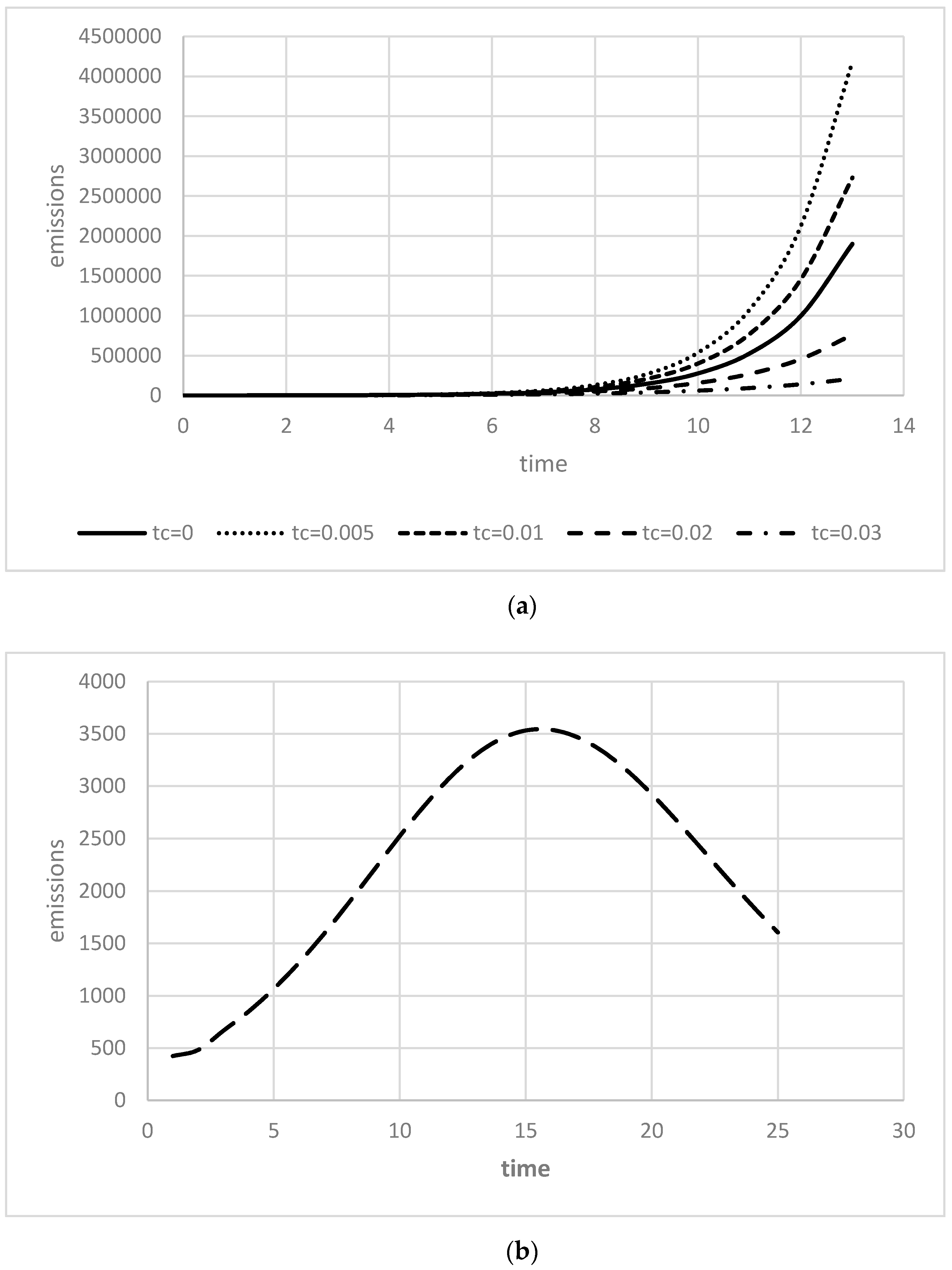
3.2. Effects of the CSTM on GHG Emissions

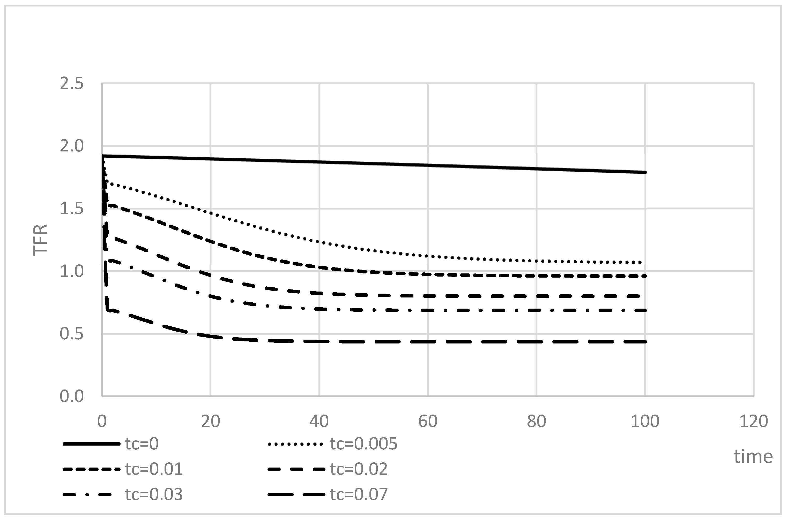
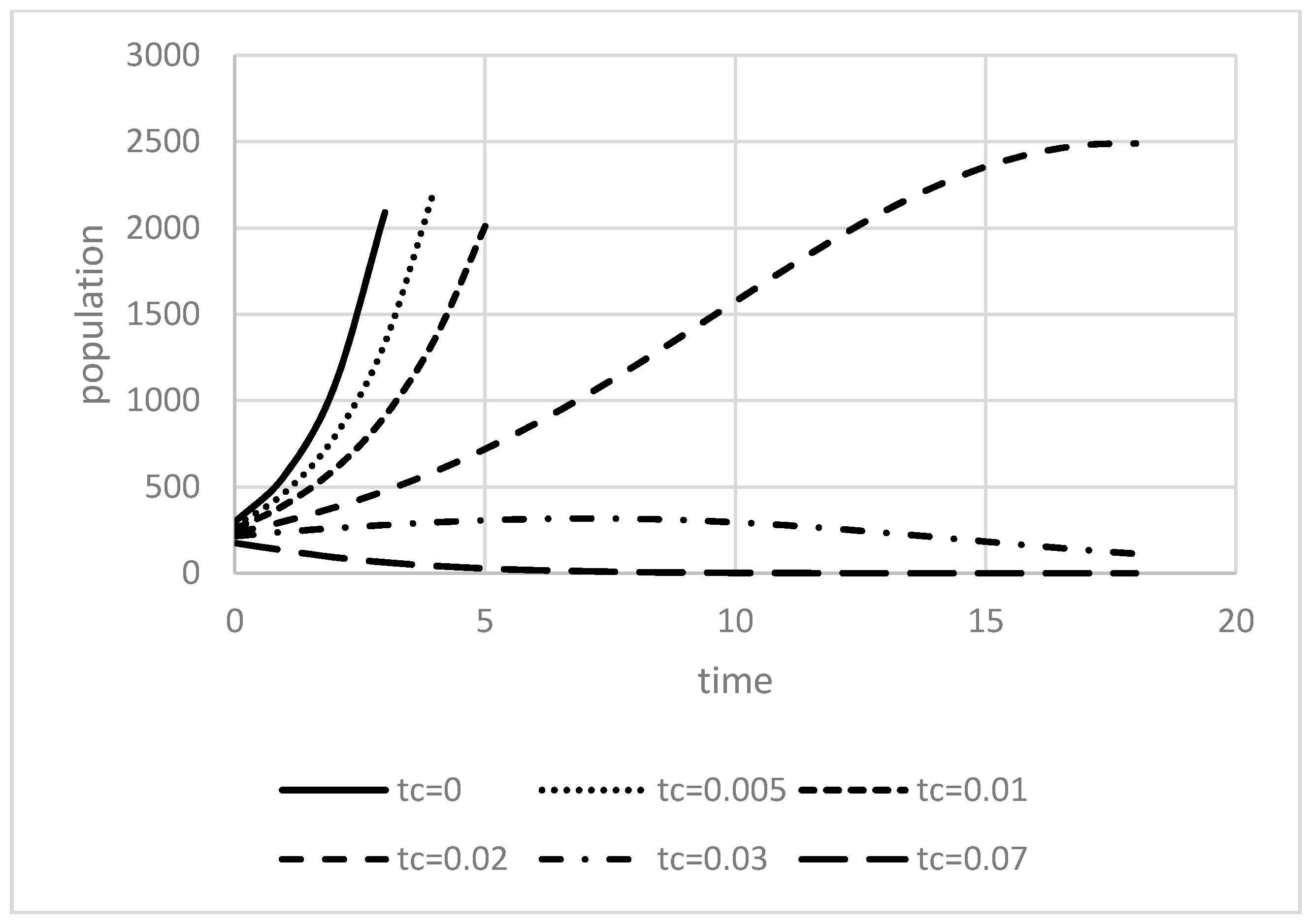
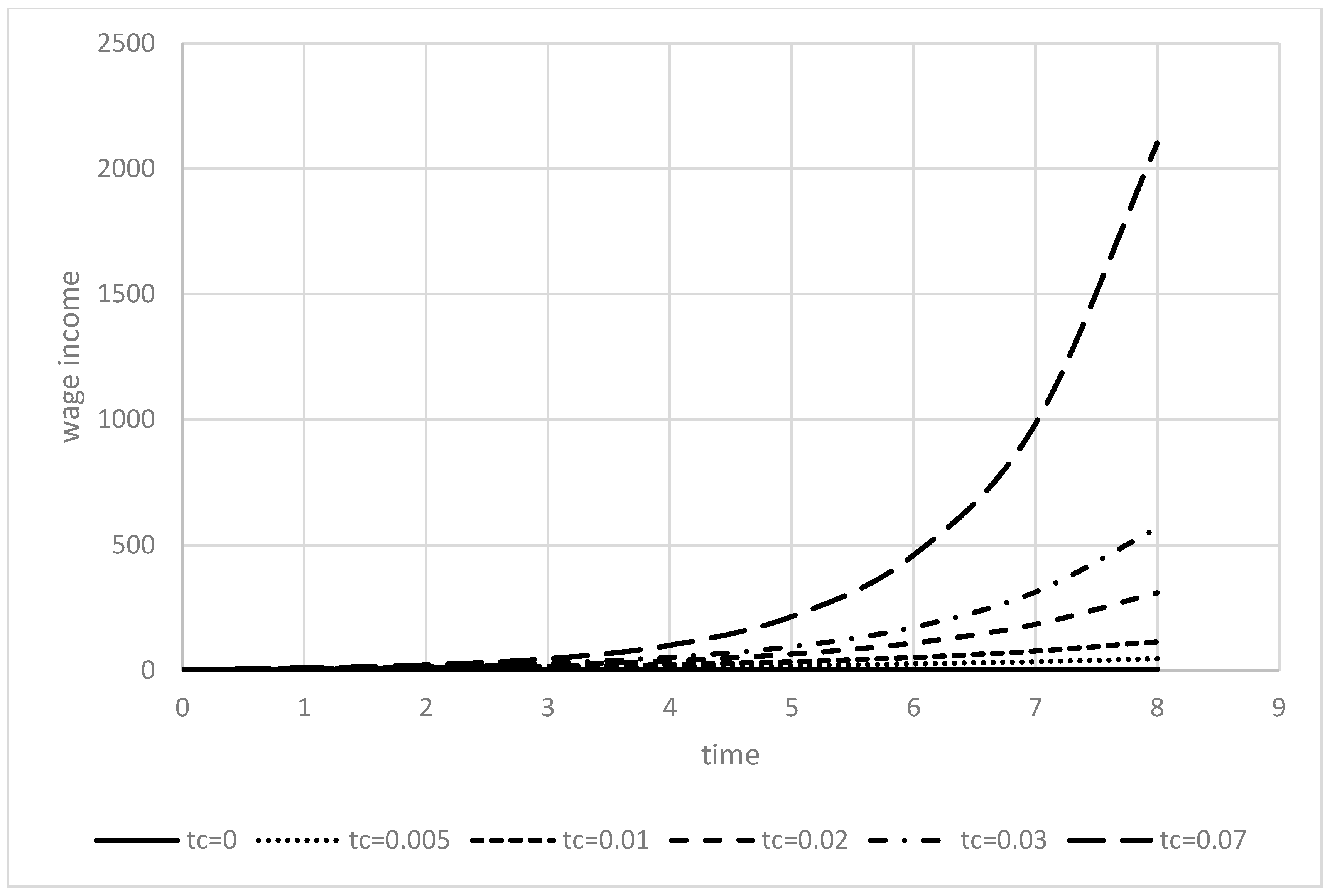
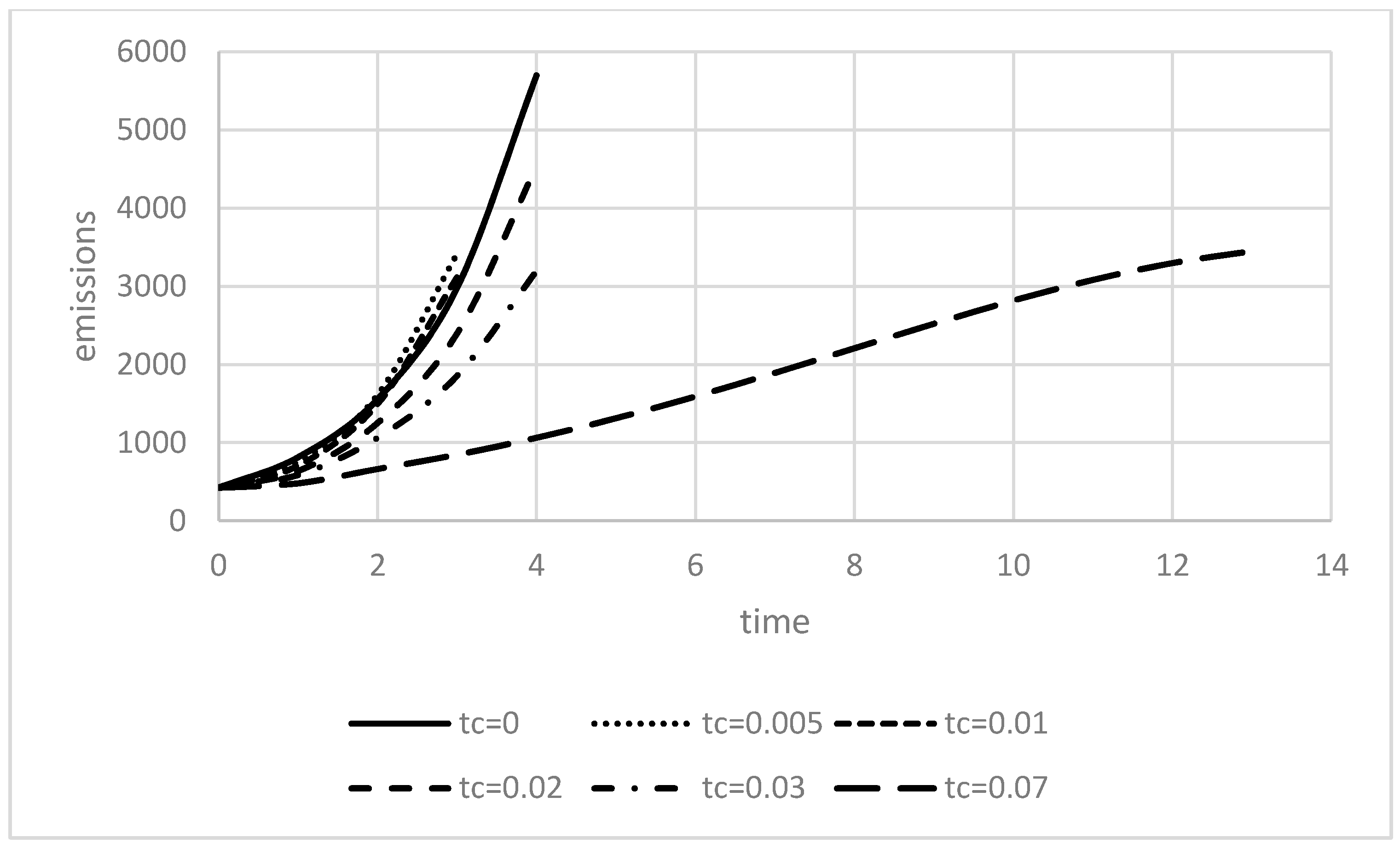
Regarding the GHG emissions $I_t$ of the economy, we refer to a modified IPAT model. The model was originally introduced by Ehrlich and Holdren [44], where I represents the environmental impact, P the population, A per capita activity and T the technology, that can be interpreted as impact per unit of activity. The argument is that, GHG emissions depend both on production and consumption decisions of individuals, which include, inter alia, the space used for living (land-use change), the household size, the treatment of waste materials, the awareness level of environmental problems, or willingness to buy environmentally friendly products. According to Dietz and Rosa [10], the per capita production can be interpreted as the affluence or activity per capita but the definition of technology is somewhat difficult. In the literature [17,18,21,109,110,111], technology is measured through the CO₂ intensity (CO₂ emissions per monetary unit of GDP) or energy intensity (energy consumption per unit of GDP), which is negatively affected by human capital. On average the CO₂ intensity (kg of CO₂ per PPP-$2011) declined by 3.5% pa and in total by 57% between 1990 and 2014. The world average energy intensity (mega joule per PPP-$2011) decreased by 1.5% pa and in total by 30% in the same period. On one hand, human capital is responsible for developing new production technologies, which increase the labor productivity and hence production. On the other hand, human capital is also responsible for an improving awareness of environmental issues and for the development of environmentally friendly technologies, which increase the environmental efficiency of production. To illustrate the effect caused by human capital, we consider as an example a new central processing unit (CPU), which requires less energy but works faster than older CPUs. We assume that a 1% increase of the per capita human capital increases the GHG emissions by $\eta$%, caused by an increasing per capita output (effect of affluence) and simultaneously decreases the GHG emissions by $\xi$%, caused by a more environmental friendly production method (effect of technology). In total the GHG emissions will change by $\left(\eta -\xi \right)$% if the per capita human capital stock increases by 1%. The GHG emissions are represented by $I_t$, and these are determined by the following function:

$$I_t=\Psi {\left(y_t{h}_t{D}_t\right)}^{\eta }{\left(P_t\right)}^{\delta }{\left(h_t\right)}^{-\xi }=\Psi {\left(y_t{D}_t\right)}^{\eta }{\left(P_t\right)}^{\delta }{\left(h_t\right)}^{\gamma }$$

(28)

where $\Psi ,\eta ,\delta ,\xi >0$, $\eta -\xi =\gamma$ and $P_t$ is the total population alive in period t

$$P_t=N_t+N_{t+1}+\rho \left(h_{t-1}\right)N_{t-1}=N_t\left(1+n_t+\frac{\rho \left(h_{t-1}\right)}{n_{t-1}}\right)$$

(29)

Obviously, the effect on emissions caused by a change of one of the variables depends strongly on the parameter values of $\eta , \delta ,$ and $\xi$. Several studies attempt to estimate these parameters. Liddle [109] considered the outcomes of 18 other studies and concluded that the parameter measuring the elasticity of emissions with respect to population size $\delta$ is not robust over time and not significantly different from unity. However, he [109] states that the elasticity of emissions with respect to per capita income is highly robust over time for OECD countries and at most unity.

Most studies [17,18,19,55,111,112,113] find that the impact of population exceeds the impact of output per capita. Shi [19] concluded from different approaches that the impact of a 1% increase of population results in increase of CO₂ emissions in the range of 1.4–1.6%. All studies agree that population growth has the strongest effect on CO₂ emissions. Casey and Galor [114] recently derived that a move from the medium to the low variant of UN fertility projections will be associated with a 35% decline in the yearly GHG emissions and 15% higher income per capita.

Therefore, we assume conservatively that $\eta \le 1$ and $\delta =1$. For simplicity, we assume that the life expectancy is fixed and hence the fertility rate remains constant in time, ceteris paribus. Thus, the population size can be written as:

$$P_t=N_t+N_{t+1}+\rho \left(h_{t-1}\right)N_{t-1}=N_1\left(n^{t-1}+n^t+\rho n^{t-2}\right)$$

(30)

with $n=\frac{\varphi \left(1-\psi m\right)}{\left(e+{\tau }^c\right)\left(1+\chi \rho +\varphi \right)}$.

The impact of the CSTM is analyzed by differentiating the total emissions with respect to ${\tau }^c$, where we assume that the CSTM is introduced in t = 1 and remains unchanged. According to the assumptions made above, the GHG emissions per period of this economy is given by:

$$I_t=\Psi {\left(y{\left(1-d\right)}^t{D}_0\right)}^{\eta }{N}_1\left(\left(n^{t-1}+n^t+\rho n^{t-2}\right)\right){\left(h_1{\left(\Omega {\left(\frac{\psi m\left(e+{\tau }^c\right)}{\left(1-s_h\right)\left(1-\psi m\right)}\right)}^m\right)}^{t-1}\right)}^{\gamma }$$

(31)

Differentiating Equation (30) with respect to the tax rate delivers:

$$\frac{\partial I_t}{\partial {\tau }^c}=\frac{I_t}{{\tau }^c}\left(\gamma \left(t-1\right)\underset{{\epsilon }_{G^h,{\tau }^c}}{\underbrace{\left(\frac{m{\tau }^c}{em\psi +{\tau }^c}\right)}}\underset{{\epsilon }_{n,{\tau }^c}}{\underbrace{-\left(\frac{{\tau }^c}{e+{\tau }^c}\right)}}\left(t-\frac{n^{t-1}+2\rho n^{t-2}}{n^{t-1}+n^t+\rho n^{t-2}}\right)\right)$$

(32)

where ${\epsilon }_{G^h,{\tau }^c}$ represents the elasticity of human capital with respect to the CSTM, and ${\epsilon }_{n,{\tau }^c}$ represents the elasticity of the number of children with respect to the CSTM. Obviously, the emissions will decline if the following holds:

$$\gamma <\frac{em\psi +{\tau }^c}{m}\left(\frac{\left(t-\frac{n^{t-1}+2\rho n^{t-2}}{n^{t-1}+n^t+\rho n^{t-2}}\right)}{\left(t-1\right)}\right)$$

(33)

Because of the fact that the CSTM is recommended for countries with fertility rates above the sustainable level (in this model, the sustainable quantity is one child), the second multiplier on the right-hand side is always at least one. By choosing an appropriate tax rate, the first multiplier also exceeds one. On the other hand, as noted earlier, it is reasonable to assume that $\gamma$ lies in the range of zero and one. This condition is usually fulfilled.

Proposition 5.

The introduction or extension of the CSTM will lead to a reduction of emissions, if the child-tax rate and the child-subsidy rate are sufficiently high.

We can conclude that the above proposed mechanism is able to increase the growth of income, reduce population and reduce emissions. In the next section, we calibrate the consequences of the mechanism with reference to an aging economy.

4. Calibration

As described in Equation (8), the life expectancy depends on the human capital that a person acquires at a young age. This means that the effect of the child-subsidy child-tax mechanism on the population size in Equation (28) will be alleviated, but it is unclear if the characteristics of the CSTM will remain unchanged.

To examine this, we calibrate the model so that the outcomes are clear in the case of no CSTM in the first period under consideration. The precise values are presented in the Appendix A. For the human capital growth rate, we get a value of 0.01–0.012% pa (The value depends on the assumed number of years per life period. We have used 25 and 30 years per period), and this range of values coincides with the growth rates of human capital for developing countries calculated from the data provided by Lee and Lee [115]. The total fertility rate is 1.92 children per individual. This coincides with just 3.84 children per female in reality. The initial value of the life expectancy is assumed to be 0.16, which results in an expected life time between 54 and 65 years. The loss of labor productivity caused by climate change is assumed to be 0.03% per period. The remaining initial values for emissions, number of workers, and wage rate are taken arbitrarily. Taking these assumptions, we consider six tax rates for the CSTM, 0 (representing the BAU scenario), 0.5%, 1%, 2%, 3%, and 7%. Taking these assumptions, we get the following diagrams for the fertility rate, the population, the emissions and the wage income, where the latter can be taken as an indicator for the per capita income or economic development.

In Figure 1, the development of the fertility rate is represented. In the BAU scenario (the solid line), the fertility rate decreases slightly and this decline is caused by the increasing life expectancy. The application of the CSTM from period one onwards leads to a discrete and abrupt decline of the fertility rate, and the fertility declines continuously because of the increasing life expectancy.

The higher the tax rate and subsidy rate, the stronger the decline of the fertility rate. The decline of the fertility rate has consequences on the population size (Figure 2).

From Figure 2, it is clear that the population size will decline given that the tax of the CSTM rate is sufficiently high—particularly in this scenario where the tax rate is at least 2%. If the tax rate is lower, the population size will still increase but at a lower rate than in the BAU scenario.

The plots in Figure 3 confirm that more human capital leads to higher incomes. The higher the tax rate, the higher is the income. However, the income in the BAU scenario is rising only at a very modest rate close to zero.

Up to this point, the outcomes are unique. The CSTM reduces the fertility rate and population size, and increases the per capita incomes. However, with respect to emissions, a reduction will only occur if the tax rate is beyond certain threshold value (see Equation (33)) (see Figure 4a,b). In Figure 5, all 6 scenarios are presented, and it is clear that the emissions are growing relatively strongly, and that the CSMT applied with low tax rates (0.5% and 1%) leads to more emissions than in the BAU scenario. Therefore, we can derive that higher tax rates are necessary to reduce emissions.

The problem that arises with low tax rates is that the declining effect on population growth is relatively small compared to the increasing effect on growth of production. This can happen because the decline of the fertility rate is counteracted by an increase of the life expectancy rate. Even if the life expectancy remains constant, the problem can occur as indicated by the inequality Equation (33).

In contrast, in Figure 4b, which is only presenting the emission path of the scenario with a tax rate of 7%, it is noted that the emissions will decrease after some periods. In the first periods, the emissions are increasing but then they reach a maximum and thereafter strive to zero.

In summary, the CSTM will have positive economic, social, and environmental consequences. If the tax rate of the CSTM is sufficiently high, the emissions can be reduced to a sustainable level without incurring additional costs because the CSTM is tax-neutral. Moreover, considering a closed economy in which the capital stock is determined endogenously or using a production function depending on land and labor input, the outcomes changes only marginally.

5. Conclusions

In this paper, we have developed a revenue-neutral CTSM to reduce the fertility rate, to increase investments in education, to increase the per capita incomes, and reduce the emissions of less developed countries. The outcomes are at least necessary if less developed countries want to prepare for climate change and its impacts. As noted from the literature, these countries will be most affected by the consequences of climate change. At a minimum, they should have appropriate mitigation measures in place. This requires that the per capita income must increase and the population growth must decline. Given the financial restrictions that less developed countries face, it will be difficult for them to purchase advanced environmentally-friendly technologies that are used in developed countries. Therefore, much more human capital is necessary to manage the challenges caused by the consequences of climate change. The advantage of our proposal is that it is costless. Casey and Galor [114] consider Nigeria as a case and compare different population development scenarios of the United Nations. They note that a 1% slower population growth could be accompanied by an increase in income per capita of nearly 7% while still lowering carbon emissions.

Moreover, it is easy to adjust the CSTM in such a way that the first child is tax free, and that only the second and further children are taxed. Also, it is clear that a resource limited planet cannot be inhabited by an infinite number of people and there are many indications that the present world population size is beyond the sustainable level. In our view, the general underlying problem is that the negative externalities due to increase in the number of children are not well considered. Therefore, a discussion about how to internalize these externalities rarely takes place. However, we are cautious that to tax the number of children is an ethical and contentious matter.

On a more promising note, we argue that an increase in the quality of children is far more important than the quantity to achieve decent growth and avoid environmental catastrophes.

A limitation of the IPAT model that we present is the assumption we make on the parameters. Particularly, the model can be extended to address the possibility of increasing per capita incomes that can lead to an overproportional increase in consumption and/or production patterns which could be potentially harmful for the environment. Although, the case study of Casey and Galor [114] indicates that such behavioral changes are not expected, but we cannot exclude this.

Another problem is the determination of a sufficiently high tax rate, where each case has to be considered carefully by doing additionally research on reproductive and consumption behavior in the respective country.

References

1. The Paris Agreement. Available online: http://unfccc.int/paris_agreement/items/9485.php (accessed on 20 March 2019).
2. Bertoldi, P.; Ricci, A.; de Almeida, A. Energy Efficiency in Household Appliances and Lighting; Springer Science & Business Media: Berlin, Germany, 2001. [Google Scholar]
3. Dasgupta, P.; Dasgupta, A. Socially Embedded, Preferences, Environmental Externalities, and Reproductive Rights. Popul. Dev. Rev. 2017, 43, 405–441. [Google Scholar] [CrossRef]
4. Gerlagh, R.; Lupi, V.; Galeotti, M. Family Planning and Climate Change. Available online: https://www.dropbox.com/s/3djwfexr9zaexuh/GLG_2018.pdf?dl=0 (accessed on 6 March 2019).
5. Food and Agriculture Organization (FAO). How to Feed the World in 2050. Report, Geneva. Available online: http://www.fao.org/fileadmin/templates/wsfs/docs/expert_paper/How_to_Feed_the_World_in_2050.pdf (accessed on 14 February 2019).
6. Ehrlich, P.R.; Harte, J. Opinion: To feed the world in 2050 will require a global revolution. Proc. Natl. Acad. Sci. USA 2015, 112, 14743–14744. [Google Scholar] [CrossRef] [Green Version]
7. Burke, M.; Hsiang, S.M.; Miguel, E. Global non-linear effect of temperature on economic production. Nature 2015, 527, 235–239. [Google Scholar] [CrossRef]
8. Hsiang, S.M.; Sobel, A.H. Potentially Extreme Population Displacement and Concentration in the Tropics Under Non-Extreme Warming. Nat. Sci. Rep. 2015, 6, 25697. [Google Scholar] [CrossRef]
9. World Bank. Available online: https://datacatalog.worldbank.org/dataset/human-capital-index (accessed on 20 March 2019).
10. Dietz, T.; Rosa, E.A. Rethinking the environmental impacts of population, affluence and technology. Hum. Ecol. Rev. 1994, 1, 277–300. [Google Scholar]
11. Malthus, T. Essay on the Principle of Population as It Affects the Future Improvement of Society. J. Johnson in St Paul’s Church-Yard, London. Available online: https://ia802701.us.archive.org/14/items/essayonprincipl00malt/essayonprincipl00malt.pdf (accessed on 5 May 2019).
12. Ehrlich, P.R. The Population Bomb; Ballantine Books: New York, NY, USA, 1968. [Google Scholar]
13. Van Den Bergh, J.C.J.M.; Rietveld, P. Reconsidering the limits to world population: Meta-analysis and meta-prediction. Bioscience 2004, 54, 195–204. [Google Scholar] [CrossRef]
14. Daily, G.C.; Ehrlich, A.H.; Ehrlich, P.R. Optimum population size. Popul. Environ. 1994, 15, 469–475. [Google Scholar] [CrossRef]
15. Wynes, S.; Nicholas, K.A. The climate mitigation gap: Education and government recommendations miss the most effective individual actions. Environ. Res. Lett. 2017, 12, 074024. [Google Scholar] [CrossRef]
16. Zhou, Y.; Liu, Y. Does population have a larger impact on carbon dioxide emissions and income? Evidence from a cross-regional panel analysis in China. Appl. Energy 2016, 180, 800–809. [Google Scholar] [CrossRef]
17. Liddle, B.; Lung, S. Age-structure, urbanization, and climate change in developed countries: Revisiting STIRPAT for disaggregated population and consumption-related environmental impacts. Popul. Environ. 2010, 31, 317–343. [Google Scholar] [CrossRef]
18. Cole, M.A.; Neumayer, E. Examining the impact of demographic factors on air pollution. Popul. Environ. 2004, 26, 5–21. [Google Scholar] [CrossRef]
19. Shi, A. The impact of population pressure on global carbon dioxide emissions, 1975–1996: Evidence from pooled cross-country data. Ecol. Econ. 2003, 44, 29–42. [Google Scholar] [CrossRef]
20. York, R.; Rosa, E.A.; Dietz, T. STIRPAT, IPAT and ImPACT: Analytic tools for unpacking the driving forces of environmental impacts. Ecol. Econ. 2003, 46, 351–365. [Google Scholar] [CrossRef]
21. Poumanyvong, P.; Kaneko, S. Does urbanization lead to less energy use and lower CO2 emissions? A cross-country analysis. Ecol. Econ. 2010, 70, 434–444. [Google Scholar] [CrossRef]
22. Fan, Y.; Liu, L.C.; Wu, G.; Wei, Y.M. Analyzing impact factors of CO2 emissions using the STIRPAT model. Environ. Impact Assess. Rev. 2006, 26, 377–395. [Google Scholar] [CrossRef]
23. Martínez-Zarzoso, I.; Maruotti, A. The impact of urbanization on CO2 emissions: Evidence from developing countries. Ecol. Econ. 2011, 70, 1344–1353. [Google Scholar] [CrossRef]
24. Murtaugh, P.A.; Schlax, M.G. Reproduction and the carbon legacies of individuals. Glob. Environ. Chang. 2009, 19, 14–20. [Google Scholar] [CrossRef] [Green Version]
25. Nolt, J. How Harmful are the Average American’s Greenhouse Gas Emissions? Ethics Policy Environ. 2011, 14, 3–10. [Google Scholar] [CrossRef]
26. Rieder, T.N. Toward a Small Family Ethic: How Overpopulation and Climate Change Are Affecting the Morality of Procreation; Springer: New York, NY, USA, 2016. [Google Scholar]
27. Hickey, C.; Rieder, T.N.; Earl, J. Population Engineering and the Fight against Climate Change. Soc. Theory Pract. 2016, 42, 845–870. [Google Scholar] [CrossRef]
28. Becker, G.S. An economic analysis of fertility. In Demographic and Economic Change in Developed Countries; Columbia University Press: New York, NY, USA, 1960; pp. 209–240. [Google Scholar]
29. Becker, G.S.; Lewis, H.G. On the Interaction between the Quantity and Quality of Children. J. Political Econ. 1973, 81, S279–S288. [Google Scholar] [CrossRef]
30. Barro, R.J. Education and economic growth. Ann. Econ. Financ. 2013, 14, 301–328. [Google Scholar]
31. Hanushek, E. The Trade-off between Child Quantity and Quality. J. Political Econ. 1992, 100, 84–117. [Google Scholar] [CrossRef]
32. Angrist, J.; Evans, W. Children and Their Parents’ Labor Supply: Evidence from Exogenous Variation in Family Size. Am. Econ. Rev. 1998, 88, 450–477. [Google Scholar] [CrossRef]
33. Angrist, J.D.; Lavy, V.; Schlosser, A. Multiple Experiments for the Causal Link between the Quantity and Quality of Children. J. Labor Econ. 2010, 28, 773–824. [Google Scholar] [CrossRef] [Green Version]
34. Kugler, A.D.; Kumar, S. Preference for Boys, Family Size, and Educational Attainment in India. Demography 2017, 54, 835–859. [Google Scholar] [CrossRef] [PubMed] [Green Version]
35. Conley, D.; Glauber, R. Parental Educational Investment and Children’s Academic Risk Estimates of the Impact of Sibship Size and Birth Order from Exogenous Variation in Fertility. J. Hum. Resour. 2006, 41, 722–737. [Google Scholar] [CrossRef]
36. Li, H.; Zhang, J.; Zhu, Y. The quantity-quality trade-off of children in a developing country: Identification using Chinese twins. Demography 2008, 45, 223–243. [Google Scholar] [CrossRef]
37. Millimet, D.L.; Wang, L. Is the Quantity-Quality Trade-Off a Trade-Off for All, None, or Some? Econ. Dev. Cult. Chang. 2011, 60, 155–195. [Google Scholar] [CrossRef] [Green Version]
38. Rosenzweig, M.R.; Zhang, J. Do population control policies induce more human capital investment? Twins, birth weight and China’s “one-child” policy. Rev. Econ. Stud. 2009, 76, 1149–1174. [Google Scholar] [CrossRef]
39. Lee, R.; Mason, A. Fertility, human capital, and economic growth over the demographic transition. Eur. J. Popul. Rev. 2010, 26, 159–182. [Google Scholar] [CrossRef] [PubMed]
40. Huang, Y. Does A Child Quantity-Quality Trade-Off Exist? Evidence from the One-Child Policy in China. In Annual Conference 2015 (Muenster): Economic Development-Theory and Policy; (No. 113215); Socialpolitik/German Economic Association: Muenster, Germany, 2015. [Google Scholar]
41. Peters, W. Public pensions, family allowances and endogenous demographic change. J. Popul. Econ. 1995, 8, 161–183. [Google Scholar] [CrossRef]
42. Diamond, P.A. National debt in a neoclassical growth model. Am. Econ. Rev. 1965, 55, 1126–1150. [Google Scholar]
43. Stauvermann, P.J.; Kumar, R.R. Sustainability of a Pay-as-you-Go Pension System in a Small Open Economy with Ageing, Human Capital and Endogenous Fertility. Metroeconomica 2016, 67, 2–20. [Google Scholar] [CrossRef]
44. Stauvermann, P.J.; Hu, J. What can China expect from an increase of the mandatory retirement age? Ann. Econ. Financ. 2018, 19, 229–246. [Google Scholar]
45. Stauvermann, P.J.; Kumar, R.R. Demographic change, PAYG pensions and child policies. J. Pension Econ. Financ. 2017, 17, 469–487. [Google Scholar] [CrossRef]
46. Stauvermann, P.J.; Kumar, R.R. Enhancing growth and welfare through debt-financed education. Econ. Res. 2017, 30, 207–222. [Google Scholar] [CrossRef] [Green Version]
47. Shi, Y.; Zhang, J. On high fertility rates in developing countries: Birth limits, birth taxes, or education subsidies. J. Popul. Econ. 2009, 22, 603–640. [Google Scholar] [CrossRef]
48. Brock, W.A.; Taylor, M.S. Economic growth and the environment: A review of theory and empirics. In Handbook of Economic Growth; Aghion, P., Durlauf, S., Eds.; Elsevier: Amsterdam, The Netherlands, 2015; Volume 1, pp. 1749–1821. [Google Scholar]
49. Smulders, S.; Gradus, R. Pollution abatement and long-term growth. Eur. J. Political Econ. 1996, 12, 505–532. [Google Scholar] [CrossRef] [Green Version]
50. Tsur, Y.; Zemel, A. Scarcity, growth and R&D. J. Environ. Econ. Manag. 2005, 49, 484–499. [Google Scholar] [CrossRef]
51. Chu, H.; Lai, C.-C. Abatement R&D, market imperfections, and environmental policy in an endogenous growth model. J. Econ. Dyn. Control 2014, 41, 20–37. [Google Scholar] [CrossRef] [Green Version]
52. Kollenbach, G. Abatement, R&D and growth with a pollution ceiling. J. Econ. Dyn. Control 2015, 54, 1–16. [Google Scholar] [CrossRef]
53. Hirazawa, M.; Saito, K.; Yakita, A. Effects of international sharing of pollution abatement burdens on income inequality among countries. J. Econ. Dyn. Control 2011, 35, 1615–1625. [Google Scholar] [CrossRef]
54. Ehrlich, P.R.; Holdren, J.P. Impact of population growth. Science 1971, 171, 1212–1217. [Google Scholar] [CrossRef] [PubMed]
55. Dietz, T.; Rosa, E.A. Effects of population and affluence on CO2 emissions. Proc. Natl. Acad. Sci. USA 1997, 94, 175–179. [Google Scholar] [CrossRef]
56. Wei, T. What STIRPAT tells about effects of population and affluence on the environment? Ecol. Econ. 2011, 72, 70–74. [Google Scholar] [CrossRef]
57. Ecology and the Crisis of Overpopulation—Future Prospects for Global Sustainablility; Shah, A. (Ed.) Edward Elgar: Cheltenham, UK, 1998. [Google Scholar]
58. Cronshaw, M.B.; Requate, T. Population Size and Environmental Quality. J. Popul. Econ. 1997, 10, 229–316. [Google Scholar] [CrossRef]
59. Dasgupta, P. Population, Resources and Poverty. Ambio 1992, 21, 95–101. [Google Scholar]
60. Dasgupta, P. An Inquiry into Well-Being and Destitution; Clarendon Press: Oxford, UK, 1993. [Google Scholar]
61. Dasgupta, P. The Population Problem: Theory and Evidence. J. Econ. Lit. 1995, 33, 1879–1902. [Google Scholar]
62. Dasgupta, P. Population, Resources, and Welfare: An Exploration into Reproductive and Environmental Externalities. In Handbook of Environmental Economics: Environmental Degradation and Institutional Responses; Maler, K.-G., Vincent, J., Eds.; Elsevier: Amsterdam, The Netherlands, 2003; Volume 1, pp. 191–247. [Google Scholar]
63. Nerlove, M. Population and the Environment: A Parable of Firewood and Other Tales. Am. J. Agric. Econ. 1991, 73, 1334–1347. [Google Scholar] [CrossRef]
64. Nerlove, M.; Meyer, A. Endogenous Fertility and the Environment: A Parable of Firewood. In The Environment and Emerging Development Issues; Dasgupta, P., Maler, K.-G., Eds.; Clarendon Press: Oxford, UK, 1997; pp. 259–282. [Google Scholar]
65. Kelly, D.L.; Kolstad, C.D. Malthus and Climate Change: Betting on a Stable Population. J. Environ. Econ. Manag. 2001, 41, 135–161. [Google Scholar] [CrossRef] [Green Version]
66. Harford, J.D. Stock Pollution, Child-Bearing Externalities, and the Social Discount Rate. J. Environ. Econ. Manag. 1997, 33, 94–105. [Google Scholar] [CrossRef]
67. Harford, J.D. The Ultimate Externality. Am. Econ. Rev. 1998, 88, 260–265. [Google Scholar]
68. Harford, J.D. Methods of Pricing Common Property Use and Some Implications for Optimal Child-Bearing and the Social Discount Rate. Resour. Energy Econ. 2000, 22, 103–124. [Google Scholar] [CrossRef]
69. Becker, G.S.; Barro, R.J. A reformulation of the economic theory of fertility. Q. J. Econ. 1988, 103, 1–25. [Google Scholar] [CrossRef]
70. Barro, R.J.; Becker, G.S. Fertility choice in a model of economic growth. Econometrica 1989, 57, 481–501. [Google Scholar] [CrossRef]
71. Tomasevski, K. The State of Right to Education Worldwide: Free or Fee: Global Report 2006. Available online: http://www.katarinatomasevski.com/images/Global_Report.pdf (accessed on 6 March 2019).
72. Jost, F.; Quaas, M. Environmental and population externalities. Environ. Dev. Econ. 2010, 15, 1–19. [Google Scholar] [CrossRef]
73. Bohn, H.; Stuart, C. Calculation of a Population Externality. Am. Econ. J. Econ. Policy 2015, 7, 61–87. [Google Scholar] [CrossRef] [Green Version]
74. Stern, N. The Economics of Climate Change: The Stern Review; Cambridge University Press: Cambridge, MA, USA, 2006. [Google Scholar]
75. Graff Zivin, J.; Neidell, M. Temperature and the allocation of time: Implications for climate change. J. Labor Econ. 2014, 13, 1–26. [Google Scholar] [CrossRef]
76. Schlenker, W.; Roberts, M.J. Non-linear temperature effects indicate severe damages to U.S. crop yields under climate change. Proc. Natl. Acad. Sci. USA 2009, 106, 15594–15598. [Google Scholar] [CrossRef] [PubMed]
77. Forzierie, G.; Bianchi, A.; Batista e Silva, F.; Herrerad, M.A.M.; Lebloise, A.; Lavallec, C.; Aerts, J.C.J.H.; Feyen, L. Escalating impacts of climate extremes on critical infrastructures in Europe. Glob. Environ. Chang. 2018, 48, 97–107. [Google Scholar] [CrossRef] [PubMed]
78. Hsiang, S.M. Temperatures and cyclones strongly associated with economic production in the Caribbean and Central America. Proc. Natl. Acad. Sci. USA 2010, 107, 15367–15372. [Google Scholar] [CrossRef] [Green Version]
79. Hsiang, S.M.; Kopp, R.; Jina, A.; Rising, J.; Delgado, M.; Mohan, S.; Rasmussen, D.J.; Muir-Wood, R.; Wilson, P.; Oppenheimer, M.; et al. Estimating economic damage from climate change in the United States. Science 2017, 356, 1362–1369. [Google Scholar] [CrossRef] [Green Version]
80. Hsiang, S.M.; Jina, A.S. The Causal Effect of Environmental Catastrophe on Long-Run Economic Growth: Evidence from 6700 Cyclones; NBER Working Paper No. 20352; National Bureau of Economic Research: Cambridge, MA, USA, 2014. [Google Scholar]
81. Arnell, N.; Lloyd-Hughes, B. The global scale impacts of climate change on water resources and flooding under new climate and socioeconomic scenarios. Clim. Chang. 2013, 122, 127–140. [Google Scholar] [CrossRef]
82. Schewe, J.; Heinke, J.; Gertena, D.; Haddelandc, I.; Arnell, N.W.; Clarke, D.B.; Dankers, R.; Eisner, S.; Feketeh, B.M.; Colón-González, F.J.; et al. Multimodel assessment of water scarcity under climate change. Proc. Natl. Acad. Sci. USA 2014, 111, 3245–3250. [Google Scholar] [CrossRef]
83. Hinkel, J.; Lincke, D.; Vafeidis, A.T.; Perrette, M.; Nicholls, R.J.; Tol, R.S.J.; Marzeion, B.; Fettweis, X.; Ionescu, C.; Levermann, A. Coastal Flood Damage and Adaptation Costs under 21st Century Sea Level Rise. Proc. Natl. Acad. Sci. USA 2014, 111, 3292–3297. [Google Scholar] [CrossRef] [PubMed]
84. Pycroft, J.; Abrell, J.; Ciscar, J.C. The Global Impacts of Extreme Sea Level Rise: A Comprehensive Economic Assessment. Environ. Resour. Econ. 2015, 64, 225–253. [Google Scholar] [CrossRef]
85. Asuncion, R.C.; Lee, M. Impacts of Sea Level Rise on Economic Growth in Developing Asia; ADB Economics Working Paper Series No. 507; Asian Development Bank: Manila, Philippines, 2017. [Google Scholar]
86. Ciscar, J.C.; Iglesias, A.; Feyen, L.; Szabóa, L.; Van Regemortera, D.; Bas Amelung, B.; Nicholls, R.; Watkiss, P.; Christensen, O.B.; Dankers, R.; et al. Physical and economic consequences of climate change in Europe. Proc. Natl. Acad. Sci. USA 2011, 108, 2678–2683. [Google Scholar] [CrossRef] [PubMed] [Green Version]
87. Carlton, T.A.; Hsiang, S.M. Social and economic impacts on climate. Science 2016, 353. [Google Scholar] [CrossRef]
88. Dell, M.; Jones, B.F.; Olken, B.A. Temperature Shocks and Economic Growth: Evidence from the Last Half Century. Am. Econ. J. Macroecon. 2012, 4, 66–95. [Google Scholar] [CrossRef] [Green Version]
89. Deryugina, T.; Hsiang, S.M. Does the Environment Still Matter? Daily Temperature and Income in the United States; National Bureau of Economic Research Working Paper 20750; National Bureau of Economic Resesearch: Cambridge, MA, USA, 2014. [Google Scholar]
90. Colacito, R.; Hoffmann, B.; Phan, T.; Sablik, T. The Impact of Higher Temperatures on Economic Growth; Economic Brief 18-08; Federal Reserve Bank of Richmond: Richmond, VA, USA, 2018. [Google Scholar]
91. Ricke, K.L.; Caldeira, K. Maximum warming occurs about one decade after a carbon dioxide emission. Environ. Res. Lett. 2014, 9, 1–8. [Google Scholar] [CrossRef]
92. Matthews, H.D.; Caldeira, K. Stabilizing climate requires near-zero emissions. Geophys. Res. Lett. 2008, 35, 1–5. [Google Scholar] [CrossRef]
93. Solomon, S.; Plattner, G.-K.; Knutti, R.; Friedlingstein, P. Irreversible climate change due to carbon dioxide emissions. Proc. Natl. Acad. Sci. USA 2009, 106, 1704–1709. [Google Scholar] [CrossRef] [Green Version]
94. Matthews, H.D.; Solomon, S. Irreversible does not mean unavoidable. Science 2013, 340, 438–439. [Google Scholar] [CrossRef]
95. Nordhaus, W.D.; Sztorc, P. Dice 2013r: Introduction and User’s Manual. Technical Report, Yale. Available online: http://www.econ.yale.edu/~nordhaus/homepage/homepage/documents/DICE_Manual_100413r1.pdf (accessed on 6 March 2019).
96. De la Croix, D.; Doepke, M. Inequality and growth: Why differential fertility matters. Am. Econ. Rev. 2003, 93, 1091–1113. [Google Scholar] [CrossRef]
97. De la Croix, D.; Doepke, M. Public versus private education when differential fertility matters. J. Dev. Econ. 2004, 73, 607–629. [Google Scholar] [CrossRef] [Green Version]
98. De la Croix, D.; Doepke, M. To segregate or to integrate: Education politics and democracy. Rev. Econ. Stud. 2009, 76, 597–628. [Google Scholar] [CrossRef]
99. Bhattacharya, J.; Chakraborty, S. Fertility choice under child mortality and social norms. Econ. Lett. 2012, 115, 338–341. [Google Scholar] [CrossRef] [Green Version]
100. Cipriani, G.P. Population ageing and PAYG pensions in the OLG model. J. Popul. Econ. 2014, 27, 251–256. [Google Scholar] [CrossRef]
101. Ehrlich, I.; Lui, F.T. Intergenerational trade, longevity, and economic growth. J. Political Econ. 1991, 99, 1029–1059. [Google Scholar] [CrossRef]
102. Cutler, D.; Deaton, A.; Lleras-Muney, A. The determinants of mortality. J. Econ. Persp. 2006, 20, 97–120. [Google Scholar] [CrossRef]
103. Blackburn, K.; Cipriani, G.P. A model of longevity, fertility and growth. J. Econ. Dyn. Control 2002, 26, 187–204. [Google Scholar] [CrossRef]
104. Cipriani, G.P.; Makris, M. PAYG pensions and human capital accumulation: Some unpleasant arithmetic. Manch. Sch. 2012, 80, 429–446. [Google Scholar] [CrossRef]
105. Uzawa, H. Optimum technical change in an aggregative model of economic growth. Int. Econ. Rev. 1965, 6, 18–31. [Google Scholar] [CrossRef]
106. Lucas, R.E. On the mechanics of economic development. J. Monet. Econ. 1988, 22, 3–42. [Google Scholar] [CrossRef]
107. Azariadis, C.; Drazen, A. Threshold externalities in economic development. Q. J. Econ. 1990, 105, 501–526. [Google Scholar] [CrossRef]
108. Golosov, M.; Jones, L.E.; Tertilt, M. Efficiency with endogenous population growth. Econometrica 2007, 75, 1039–1071. [Google Scholar] [CrossRef]
109. Liddle, B. What are the carbon emissions elasticities for income and population? Bridging STIRPAT and EKC via robust heterogeneous panel estimates. Glob. Environ. Chang. 2015, 31, 62–73. [Google Scholar] [CrossRef] [Green Version]
110. Sadorsky, P. The effect of urbanization on CO2 emissions in emerging countries. Energy Econ. 2014, 41, 147–153. [Google Scholar] [CrossRef]
111. Martinez-Zarzoso, I.; Bengochea-Morancho, A.; Morales-Lage, R. The impact of population on CO2 emissions: Evidence from European countries. Environ. Resour. Econ. 2007, 38, 497–512. [Google Scholar] [CrossRef]
112. Lin, S.; Zhao, D.; Marinova, D. Analysis of the environmental impact of China based on STIRPAT model. Environ. Impact Assess. Rev. 2009, 29, 341–347. [Google Scholar] [CrossRef]
113. Harte, J. Human population as a dynamic factor in environmental degradation. Popul. Environ. 2007, 28, 223–236. [Google Scholar] [CrossRef]
114. Casey, G.; Galor, O. Is faster economic growth compatible with reductions in carbon emissions? The role of diminished population growth. Environ. Res. Lett. 2017, 12, 014003. [Google Scholar] [CrossRef] [Green Version]
115. Lee, J.-W.; Lee, H. Human Capital in the Long Run. J. Dev. Econ. 2016, 122, 147–169. [Google Scholar] [CrossRef]
Figure 1. Total fertility rate.
Sustainability 11 02585 g001
Figure 2. Population.
Sustainability 11 02585 g002
Figure 3. Wage income.
Sustainability 11 02585 g003
Figure 4. (a) Emissions with different tax rates; (b) Emissions with tax rate of 7%.
Sustainability 11 02585 g004
Figure 5. Emissions.
Sustainability 11 02585 g005