Restrictive Effects of Water Scarcity on Urban Economic Development in the Beijing-Tianjin-Hebei City Region

Abstract

This study provides a scientific assessment of water scarcity in the Beijing-Tianjin-Hebei (BTH) city region and investigates its restrictive effects on urban economic development by quantifying economic loss caused by water scarcity based on an input–output optimization model. The results show that the water scarcity reflected by shadow prices has significant sectoral and regional heterogeneities. Southern Hebei faces the most severe water scarcity in the BTH city region and the situation is worsening. Water scarcity is shown to have a negative impact on the economy of the BTH city region that amounts to CNY 270.02 billion. Hebei has the largest potential economic loss caused by water scarcity, especially in southern Hebei, the potential GDP (gross domestic product) of which is decreased by 6.2%. This study also points out that the water scarcity in the BTH city region is underestimated in terms of actual water prices, and the scarcity of agricultural water use is mostly underestimated. The results contribute to a deeper understanding of the restrictive impact of water scarcity on regional economic development, and thus provide a scientific reference for policymaking in the BTH city region.

1. Introduction

Given the tremendous increase in water demand, also accompanied by population expansion, rapid urbanization, as well as economic booms, the issue of water scarcity has intensified and is now jeopardizing food security, regional stability, and sustainable development in many areas [1,2,3,4]. Currently, an estimated 3.6 billion people (almost half of the global population) live in areas that may face water scarcity for at least one month each year, and this number may increase to around 4.8–5.7 billion by 2050 [5]. In this context, a major challenge for governments is to enable the supply of water for domestic consumption in urban communities located in semi-arid environments, such as California, Brazil, the Middle East, and northern China [6], where the economic impacts of water scarcity are increasing [7,8]. China is, thus, a country under great pressure from water shortages, with its per capita occupancy of water resources being 2074.5 m³ in 2017 [9], less than a quarter of the world average level. The Beijing-Tianjin-Hebei (BTH) city region in northern China faces the most severe water shortages [10].

An assessment of water scarcity is fundamental for water management, since it allows policymakers to become aware of the severity of the problem [11,12]. Amber [13] and Pedro-Monzonís [14] provided basic reviews of water scarcity and drought from different perspectives to assess the state of the water recovery system to better manage water resources under water scarcity conditions and to help decision makers and stakeholders select the most appropriate indicators. Kummu [15] analyzed the temporal development of physical, population-driven water scarcity using population data derived from the History Database of the Global Environment (HYDE) dataset. Hoekstra [16] assessed freshwater scarcity using the blue footprints of 405 river basins over the period of 1996–2005, showing that for 201 basins with 2.67 billion inhabitants there was severe water scarcity during at least one month of the year. Gain [17] provided a comprehensive dynamic assessment of the water scarcity risks for the Lower Brahmaputra river basin, with the results indicating that the risk of water shortage was expected to increase slightly and fluctuate significantly with the change of the danger signal.

Water price is an effective indicator of water scarcity. Theoretically, water price should be determined based on both the supply and demand of water resources under perfect market conditions, and thus measure the real value of water resources. However, in reality, water price usually deviates from its real value, since it is top-down administratively determined, rather than on the market [18]. As such, the water shadow price is defined as the marginal contribution of unit water resources to social and economic development after the optimized allocation, which makes it a scientific and reasonable measure of the real value and scarcity of water resources [19]. The water shadow price is typically calculated using linear programming techniques [20,21]. Liu [22] calculated the shadow prices of industrial and productive water in nine river basins using input–output tables for water conservancy in combination with linear programming techniques, pointing out that the shadow price was a valuable tool for setting reasonable water prices and establishing a water market in China. Input–output models can, thus, fully consider the relationships between the various sectors but cannot calculate shadow prices in consecutive years due to data limitations.

As such, if we want to examine the shadow prices of consecutive years, Data Envelopment Analysis (DEA) is a better choice [23]. For example, Shen [24] estimated the shadow price and technical efficiency of agricultural water by a stochastic nonparametric envelopment of a data model (StoNED), which combined DEA with the Stochastic Frontier Approach (SFA). Wang [25] used the Global Non-radial Distance Function (GNDF) to measure the shadow price of industrial water during 2004–2012. Recently, the distance production function has become widely used in shadow price calculations. Zhang [26] and Wang [27], respectively, derived the shadow prices of China’s carbon emissions at provincial levels and industrial levels by using the directional output distance function. Tang [28] and Färe [29] used the directional output distance function to calculate the shadow price of agricultural sectors in China and the United States. This method allows the production modeling of a multi-input and multi-output technology when the prices of some outputs or inputs are not available, or alternatively when the prices are available but cost, profit, or revenue representations are precluded because of the possibility of violations of the required behavioral assumptions of cost minimization or profit maximization [30]. However, existing studies on shadow price for production water at the city level and the shadow price of water for the service sector are still rare. In addition, it is also hard to calculate the shadow price of water for the three major industries (i.e., agriculture, industry, and service sector) in a region simultaneously.

Given the conflict between limited water endowment and the rising water demand driven by socio-economic development, the restrictive impact of water resources has attracted increasing attention. Liu [31] analyzed the impact of water resources on regional economic growth based on the Cobb-Douglas production function, and found that the loss of economic growth caused by water scarcity was mainly due to industrial structure, technological progress, water saving, and scarcity of water resources. To measure the constraint effect of water scarcity on economic growth, some scholars calculated the “drag effect” of water use on economic growth by embedding water as a production resource into the Cobb-Douglas production function. The Cobb-Douglas production function, including natural resources and land, constructed by Romer [32] revealed the differences between unlimited and limited economic growth due to water scarcity [33,34,35]. Romer [32] argued that the growth drag caused by resources and land limitations was the difference between the growth in a hypothetical case of equilibrium development and that in the case of these limitations.

Similar analytical thinking is often used in examining the effects of specific policies and actions on society and the economy by comparing various scenarios under specific policies and actions with baseline scenarios [36]. The computable general equilibrium (CGE) model, combined with scenario analysis, is one of the most commonly used methods [8,37,38,39,40,41]. Bruvoll [42] applied a dynamic CGE model to measure the environmental constraints of economic growth by comparing the outcomes of the feedback model with the baseline model. Qin [40] used a multi-region CGE model to analyze the effectiveness of the measures and policies used for mitigating North China’s water scarcity with respect to three different groups of scenarios. The findings suggested that a reduction in groundwater use would negatively affect economic growth and household incomes. Based on a CGE model, Berrittella [36] investigated the role of water scarcity in the context of international trade, and the results proved that restrictions in water supply would change the trade patterns of agriculture and virtual water. Additionally, Li [43] combined the dynamic CGE model with the bio-economic model (BEM) to study the economic impact of a total water use control policy in the Heihe river basin, which was proven to have a limited negative impact on regional economic growth. Moreover, there are also studies reflecting the idea of equilibrium and investigating the economic impact of water resources using systematic methods [44,45].

The existing studies have deepened our understanding of the impacts of water resources on regional economic development, but some gaps should be noted. In most studies applying statistical methods to measure the impact of water constraint, the inter-sectoral linkages in the economic system are not fully considered. Although the CGE and social accounting matrix (SAM) can incorporate inter-sectoral linkage, they are merely applicable to analysis at large scales, such as the national or provincial levels, while the input–output model fully embodies the interconnections across all sectors in the economic system and it is applicable to city-level analyses. Considering the significant discrepancies between the 13 cities of the BTH city region in terms of economic levels and water resource endowments, it is necessary to conduct a city-level analysis on how water scarcity impacts urban economic growth.

Therefore, this study aims to address the above literature gaps using a directional output distance function and the input–output model. The objectives of this study are: (i) scientifically evaluating the scarcity of water for production in the 13 cities in the BTH city region by calculating shadow prices; and (ii) evaluating the potential economic loss caused by water scarcity in the cities of the BTH city region. The results of this study contribute to a deeper understanding of the water scarcity in the BTH city region and its restrictive impact on urban economic growth, and thus provide a scientific reference for policymaking in the BTH city region.

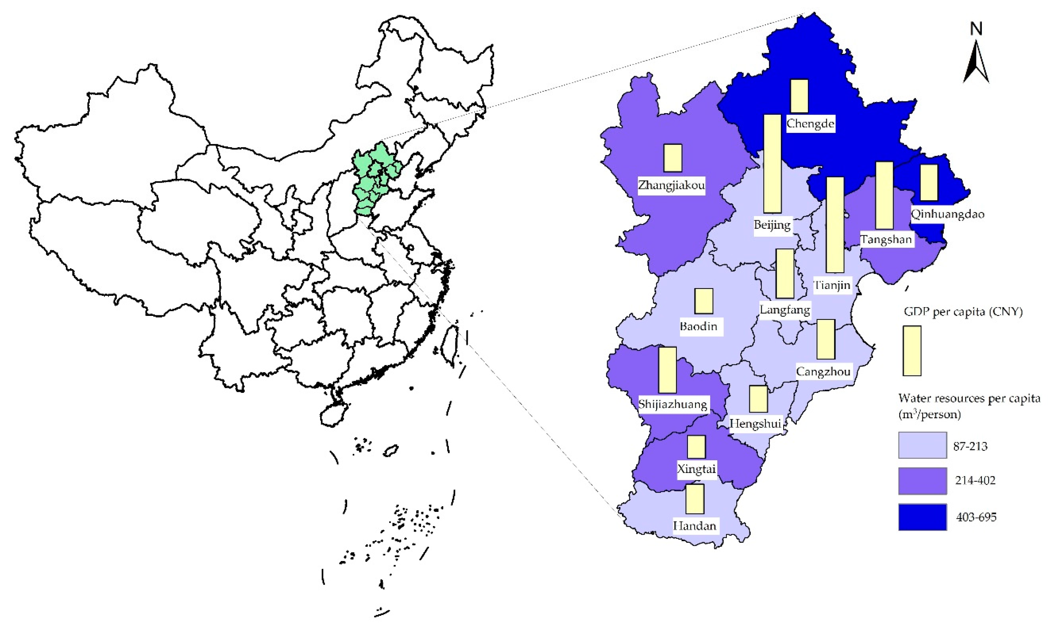
2. Background of BTH

The BTH city region is composed of 13 cities, including Beijing, Tianjin, and 11 cities in Hebei (Figure 1). The region lies at the core of China’s Circum-Bohai-Sea region, which occupied 1.9% of China’s territory, had 8.09% of the nation’s population, and produced 9.77% of China’s GDP, as of 2017 [9]. The past two decades have witnessed rapid economic growth and sustained population expansion in the region. During 2000–2017, the total GDP of the BTH city region increased from CNY 995.86 billion to 8058.05 billion, for an average annual growth rate of 13.06%. Meanwhile, its total population increased from 90.39 million to 112.47 million, with an average annual growth rate of 1.4% [9,46]. However, the region is extremely water scarce, with average annual water resources amounting to only 18.11 billion m³, that is, 0.63% of the national total water resources. The per capita occupancy of water resources in the region is 161.02 m³/capita per year, only 7.76% of the national average level, and far lower than the international standard water shortage limit of 1000 m³/capita per year [8]. Additionally, the average proportion of agricultural water use is as high as 75%, which is not favorable for regional water conservation [47,48,49]. Worse, the extent of water scarcity in the region is usually underestimated, resulting in large economic loss and waste of water resources. In this context, it is necessary to scientifically evaluate the levels of water scarcity in the cities of the BTH city region and determine to what extent water scarcity restricts urban economic development.

There is a distinct heterogeneity amongst the cities in the BTH city region in terms of economic level and water resource constraints (Figure 1,

Table 1. The economic and production water use condition in the BTH city region (Year 2016).

Regions/Cities		Economic Condition			Water Endowment Condition		Water Use Condition
		GDP Per Capita (CNY/person)	The Per Capita Net Income of Rural Residents (CNY)	The Per Capita Disposable Income of Urban Residents (CNY)	Total Water Resources (108m3)	Water Resources Per Capita (m3/person)	Residential Water Use Per Capita (m3/person)	Agricultural Water Use Per Capita (m3/person)	Industrial Water Use Per Capita (m3/person)	Services Water Use Per Capita (m3/person)
Beijing	-	11813.2	22310.0	57275.0	35.1	161.5	34.1	44.9	23.7	43.2
Tianjin	-	11449.3	20076.0	37110.0	18.9	121.0	25.4	82.8	37.9	7.9
Northern Hebei	Zhangjiakou	3312.9	9241.0	26069.0	17.8	402.3	22.0	182.4	31.8	2.3
	Chengde	4074.4	8736.0	24856.0	24.0	679.5	30.3	181.1	40.2	7.7
	Qinhuangdao	4359.2	11621.0	30348.0	21.5	694.8	29.6	197.6	51.1	7.6
	Sub-total/average	3693.7	8988.5	25462.5	41.8	540.9	26.8	186.2	39.8	5.5
Central Hebei	Langfang	5893.8	14286.0	34633.0	7.1	153.9	28.7	150.5	33.5	6.0
	Cangzhou	4723.2	11340.0	28605.0	6.5	86.6	22.3	136.4	27.7	1.8
	Tangshan	8102.1	15023.0	33725.0	22.4	285.6	32.5	207.2	79.0	14.2
	Baoding	2988.5	11612.0	25680.0	24.8	213.2	22.2	214.1	23.3	4.6
	Sub-total/average	5426.9	13065.3	30660.8	60.8	184.8	25.8	184.8	39.7	6.5
Southern Hebei	Shijiazhuang	5496.7	12345.0	30459.0	32.0	296.7	28.7	224.4	34.6	7.1
	Handan	3540.6	12153.0	26603.0	17.9	188.6	23.4	163.5	32.8	1.7
	Xingtai	2699.5	10006.0	23913.0	25.6	349.7	23.0	193.8	27.4	0.8
	Hengshui	3188.8	10069.0	23787.0	6.5	146.0	19.6	306.1	29.2	2.4
	Sub-total/average	3731.4	11143.3	26190.5	82.0	245.2	24.5	210.7	31.7	3.4
Regional Total/Average		5606.9	13099.8	31059.6	238.6	257.0	27.1	152.2	34.1	12.7

Data source: Hebei economic yearbook 2017 [50]; Water resources bulletin of Beijing, Tianjin, and Hebei 2012, 2016 [47,48,49].

). Beijing is the most economically developed, with the highest GDP and income per capita, followed by Tianjin and Hebei. It is worth noting that the economic levels and water resources are discrepant, even inside Hebei. Cities (except for Baoding) in central Hebei generally have the highest economic levels, while their water resources are scarcest. Specifically, the water scarcity in Cangzhou is extreme, with water resources of merely 86.6 m³ per capita. Except for Shijiazhuang, the other three cities in southern Hebei (i.e., Handan, Xingtai, and Hengshui) have both low economic levels and water resources endowments, with GDPs and income per capita below the average province level and water resources per capita below 200 m³. The water resource constraint in the cities in northern Hebei is lightest, with water resources per capita mostly over 500 m³, much higher than any other cities in the BTH city region. Different levels of economic development and water resources have led to large differences in water use between cities. Due to limited data on sub-industries, we calculate the water use conditions of different sectors for 2012, as listed in Table 1. Beijing has the highest per capita residential water use (34.1 m³/person) and per capita services water use (43.2 m³/person) and the lowest per capita agricultural water use (44.9 m³/person) and per capita industrial water use (23.7 m³/person). The per capita agricultural water use (82.8 m³/person) in Tianjin is significantly lower than that in the cities of Hebei, while the per capita services water use (7.9 m³/person) is higher than that in Hebei. Although the per capita water use gap of the various industries is relatively small inside Hebei, the per capita agricultural water use (201.7 m³/person) in southern Hebei is higher and the per capita water consumption in other sectors is lower. Given the non-negligible city-level differences, it is necessary to conduct a city-level analysis on water scarcity and its restrictive impact on urban economic growth.

3. Data and Methodology

3.1. Data

The calculation of the shadow price of water resources includes input variables (capital, labor, and water use) and an output variable (industrial value added). Considering data availability, the analysis period is 2000–2016. Since the shadow prices of water resources in this study are categorized into agricultural, industrial, and service sector water shadow prices, the above four variables also have to be categorized by the three industries. Furthermore, the labor input is represented by the number of employees in each sector and capital data are estimated based on existing studies on the capital stock estimation of industries [51,52,53]. The basic data on the above three input variables are derived from the Beijing Statistical Yearbook, Tianjin Statistical Yearbook, and Hebei Economic Yearbook for 2001–2017 [54,55,56]. Water resource inputs are represented by direct water withdrawal from each sector, which is estimated based on data from the Beijing Water Resources Bulletin, Tianjin Water Resources Bulletin, and Hebei Water Resources Bulletin for 2000–2016 [48,49,50]. Descriptive statistics of these variables are shown in

Table 2. Descriptive statistics of input and output variables in calculation of shadow price.

Sectors	Variable	Unit	Maximum	Minimum	Mean	Standard Deviation
Agriculture	Capital	Billion CNY	16.48	0.12	3.06	34.36
	Labor	Ten thousand people	298.21	45.18	131.54	56.90
	Water	Billion ton	2.87	0.40	1.32	6.06
	Value added	Billion CNY	29.30	2.66	11.73	65.04
Industry	Capital	Billion CNY	179.06	2.12	35.41	362.02
	Labor	Ten thousand people	268.58	16.04	92.32	61.46
	Water	Billion ton	1.05	0.07	0.28	1.88
	Value added	Billion CNY	105.17	5.87	32.33	280.24
Services	Capital	Billion CNY	360.57	2.43	43.56	610.55
	Labor	Ten thousand people	1045.38	50.35	195.62	190.52
	Water	Billion ton	1.01	0.02	0.16	2.08
	Value added	Billion CNY	420.16	7.52	53.62	862.01

.

The input–output optimization modeling for the BTH city region is built based on the 2012 input–output tables of the 13 cities in the BTH city region [56,57,58].

3.2. Methodology

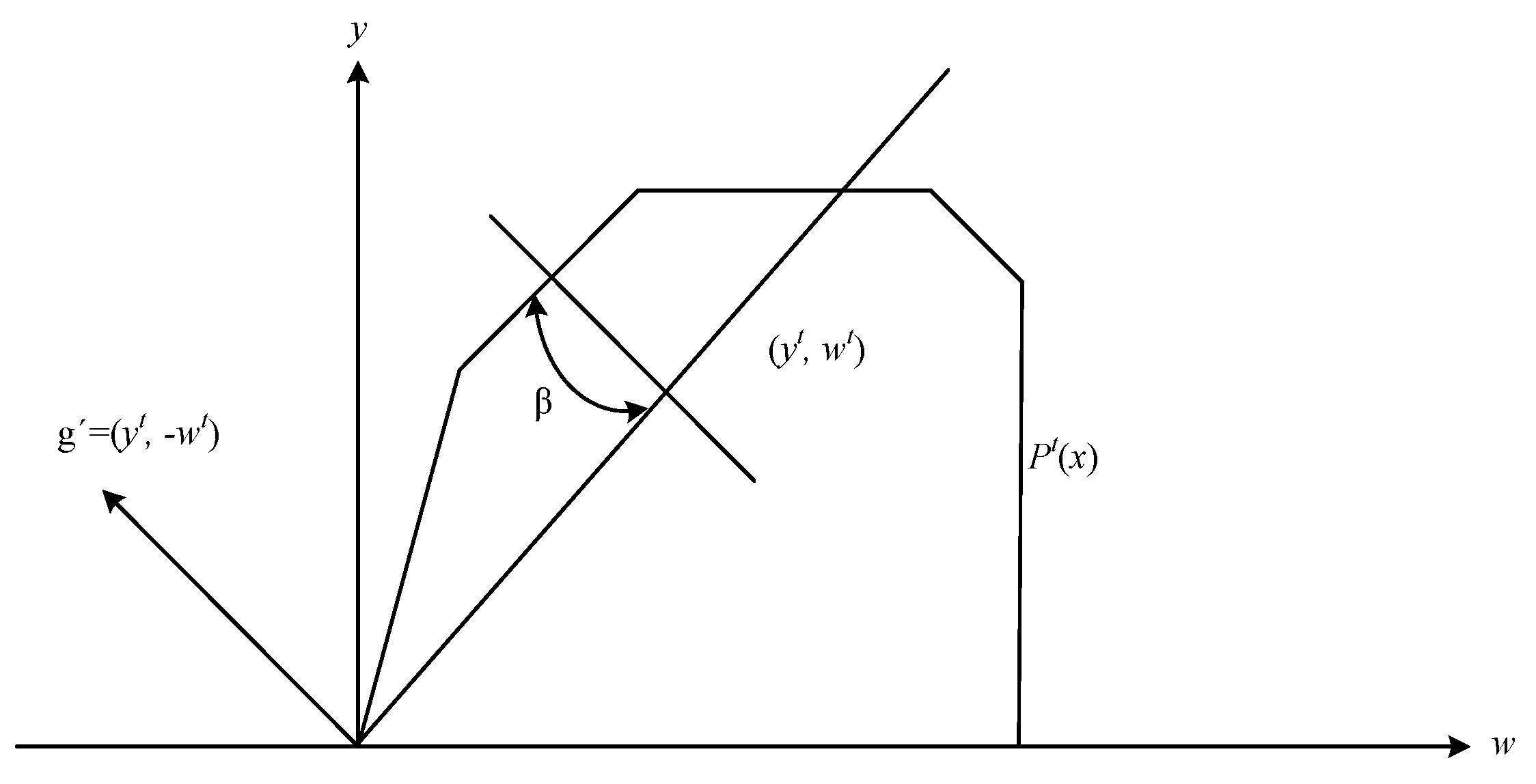
3.2.1. Calculation of Shadow Price for Production Water

This paper uses the distance output function to calculate the shadow price of production water. The theoretical model of shadow price is based on existing research studies [23,59], and the specific process is listed in the Appendix A and Appendix B.

Two techniques can be used to estimate the directional distance function: the non-parametric and the parametric approaches. The non-parametric one, namely DEA, aims to construct a piecewise frontier to encompass all DMUs (Decision Making Units). The parametric approach needs to pre-specify a function form and fit the data. This study adopts the commonly used quadratic form to represent the model empirically. A parametric specification is adopted considering its advantages of differentiability and flexibility, which enables us to easily derive the shadow price.

Specifically, the shadow price is usually calculated based on the linear mathematical programming method [19,20], but this is only a hypothesis. At present, many scholars have begun to break this limitation when solving shadow prices, and began to estimate the shadow price by means of translog production function or higher-order function [25,26,27,28]. As Färe [59] suggested, the quadratic representation over-performs compared to translog parameterizations. Following similar studies [25,26,27,28], we set the directional distance function to quadratic, with the direction vector of $(g_y,g_w)=(1,-1)$. This means that while other inputs remain unchanged, output increases and water use decreases can be achieved at the same time. Assuming the number of the cities is k $(k=1,2,\cdots ,13)$ and the number of years is t $(t=1,\cdots ,17)$, the quadratic directional distance function for city k in year t is given as:

$$\begin{array}{c}\overrightarrow{D_k^t}(x_k^t,y_k^t,w_k^t;1,-1)=\mathsf{\alpha }+{\displaystyle \sum _{n=1}^2{\mathsf{\alpha }}_n{x}_{nk}^t}+{\mathsf{\beta }}_1{y}_k^t+{\mathsf{\gamma }}_1{w}_k^t+x_{nk}^t{\displaystyle \sum _{n=1}^2{\mathsf{\alpha }}_{n{n}^{\prime }}{x}_{nk}^t{x}_{n^{\prime }k}^t}+\frac{1}{2}{\mathsf{\beta }}_2{(y_k^t)}^2+\frac{1}{2}{\mathsf{\gamma }}_2{(w_k^t)}^2\\ +{\displaystyle \sum _{n=1}^2{\mathsf{\eta }}_n{x}_{nk}^t{w}_k^t+{\displaystyle \sum _{n=1}^2{\mathsf{\delta }}_n{x}_{nk}^t{y}_k^t}}+\mathsf{\mu }{y}_k^t{w}_k^t\hspace{1em}\hspace{1em}\hspace{1em}\hspace{1em}\end{array}$$

(1)

To estimate the parameters in the above model, we use the linear programming algorithm of Aigner [60].

Algorithm 1

$\begin{array}{l}\min {\displaystyle \sum _t{\displaystyle \sum _k\overrightarrow{D_k^t}(x_k^t,y_k^t,w_k^t;1,-1)}}\\ s.t.\\ (1) \overrightarrow{D_k^t}(x_k^t,y_k^t,w_k^t;1,-1)\ge 0\\ (2) \overrightarrow{D_k^t}(x_k^t,y_k^t,0;1,-1)\le 0\\ (3) \frac{\partial \overrightarrow{D}}{\partial w}\ge 0, \frac{\partial \overrightarrow{D}}{\partial y}\le 0, \frac{\partial \overrightarrow{D}}{\partial x}\ge 0\\ (4) {\mathsf{\beta }}_1-{\mathsf{\gamma }}_1=-1, {\mathsf{\beta }}_2={\mathsf{\gamma }}_2=\mathsf{\mu }, {\mathsf{\delta }}_n={\mathsf{\eta }}_n\\ (5) {\mathsf{\alpha }}_{n{n}^{\prime }}={\mathsf{\alpha }}_{n^{\prime }n}\end{array}$

The objective function is to minimize the sum of the distance deviations from the frontier. Restriction (1) ensures that the production set is feasible. Restriction (2) imposes the attribute of “null-jointness.” In other words, in the extreme case of water resource consumption being zero, any non-negative output is not feasible. Restriction (3) guarantees a convex set. Restrictions (4) and (5) impose the translation and symmetry properties, respectively.

According to Färe [28], the price of output is generally considered as $p_y=1$, so the expression of the specific shadow price of water resources in this study is:

$$p_w=-\frac{{\mathsf{\gamma }}_1+{\mathsf{\gamma }}_{2}w+{\displaystyle {\sum }_{n=1}^2{\mathsf{\eta }}_n{x}_n}+\mathsf{\mu }y}{{\mathsf{\beta }}_1+{\mathsf{\beta }}_{2}y+{\displaystyle {\sum }_{n=1}^2{\mathsf{\delta }}_n{x}_n}+\mathsf{\mu }w}$$

(2)

3.2.2. Estimation of Economic Loss Caused by Water Scarcity

In this study, the restrictive impact of water scarcity on city economic growth is measured by the potential economic loss caused by water scarcity, which can be obtained by comparing the optimized GDP based on the input–output optimization model, including and excluding water constraints.

In the input–output optimization model, it is assumed that capital and labor are not constrained, which may have a certain impact on the measurement of the impact of water resources on GDP. However, the BTH city region is one of the most economically viable regions in China. Its capital and labor are abundant and the water constraint is obvious. Therefore, the effects of water resource constraints on the economic constraints measured by the input–output optimization model will not be large. In addition, the implementation of the CGE model has higher data requirements, which is difficult to obtain for Hebei’s cities. In this case, the input–output optimization model is a better choice because it can not only describe the relationships between industries in the region, but also estimates the impact of water shocks on the economy.

The input–output model is developed based on the input–output tables of the 13 cities of the BTH city region in 2012. The objective of the optimization model is to maximize the GDP of the target city, and the constraints include input–output constraints, constraints of the sectoral output in each city, and industrial water constraints. The detailed setting of the objective and constraints are as follows.

The objective is to maximize the urban economic benefit reflected by GDP. In the model setting, the relationship between sectoral output and water use is assumed as stable and can be reflected by the industrial water use coefficient. Therefore, maximizing urban GDP is achieved through the adjustment of the sectoral production scales in each city. The function for maximizing urban GDP is as follows:

$$\max {\displaystyle \sum _{R=1}^{13}{\displaystyle \sum _{i=1}^3{x}_i^R{v}_i^R}}$$

(3)

where $x_i^R$ is the output of sector i in city R and $v_i^R$ the value added rate of sector i in city R, which is the amount of added value created from one monetary unit of production.

(1) Input–Output Constraints

The input–output model is an analytical framework that represents the monetary transactions between economic sectors, and therefore, their interdependence on the economic system [61]. Its basic mathematical structure consists of n linear equations depicting how the production of an economy depends on inter-sectoral relationships and final demand:

$$x_i={\displaystyle {\sum }_{j=1}^n{x}_{ij}}+y_i,$$

(4)

where n is the number of economic sectors, $x_i$ is the total output of sector i, $x_{ij}$ denotes the inter-sectoral monetary flows from sector i to sector j, and $y_i$ is the final demand of sector i. This equation can be rewritten to include the direct input coefficient $a_{ij}$, which indicates the amount of input from sector i required to increase by one monetary unit the output of sector j, as:

$$x_i={\displaystyle {\sum }_{j=1}^n{a}_{ij}{x}_j}+y_i,$$

(5)

where

$$a_{ij}\frac{x_{ij}}{x_j},$$

(6)

Therefore, for each city, the input–output constraint can be expressed as:

$${\displaystyle {\sum }_{j=1}^n{a}_{ij}{x}_j}+y_i\le x_i,$$

(7)

(2) Constraints of Sectoral Output in Each City

To avoid dramatic fluctuations in sectoral production, the changes of sectoral outputs of each sector are assumed to be confined within a certain range:

$${\underset{\_}{x}}_i^R\le x_i^R\le {\overline{x}}_i^R,$$

(8)

where ${\underset{\_}{x}}_i^R$ and ${\overline{x}}_i^R$ are the lower and upper limits of output in sector i in city R, respectively, obtained based on the average change rate of the sectoral output in each city from 2007 to 2016 [62].

(3) Agricultural Water Constraints

The optimal agricultural water brought about by the industrial changes in each city should not exceed the actual agricultural water.

$$a_{w1}^R{x}_1^R\le W_1^R{\delta }_1^R,$$

(9)

where $a_{w1}^R$ is the agricultural water use coefficient in city R, $x_1^R$ denotes the agricultural output in city R, and ${\delta }_1^R$ indicates the change coefficient for agricultural water, which is determined by the shadow price. The change coefficient is lower in areas with severe water shortage, which means that the water constraint is stronger than the actual one. Conversely, the change coefficient is higher in areas where water shortage is not serious, but it cannot exceed 1, which means that the upper limit of agricultural water is the actual water use. $W_1^R$ indicates the actual water use in the agricultural sector of city R, the data coming from the Beijing, Tianjin, and Hebei Water Resources Bulletin (2012) [47,48,49].

(4) Industrial Water Constraints

The optimal industrial water amount brought about by the industrial changes in each city should not exceed the actual industrial water:

$$a_{w2}^R{x}_2^R\le W_2^R{\delta }_2^R,$$

(10)

where $a_{w2}^R$ is the industrial water use coefficient in city R, $x_2^R$ denotes the industrial output in city R, and ${\delta }_2^R$ indicates the change coefficient for industrial water, which is determined by the shadow price. Similar to the agricultural sector, the change coefficient ranges from 0 to 1, reflecting the degree of adjustment of water scarcity to the upper limit of water use. In areas where water scarcity is more severe, the change coefficient is lower, and conversely, the change coefficient is higher. $W_2^R$ indicates the actual water use in the industrial sector in city R, the data coming from the Beijing, Tianjin, and Hebei Water Resources Bulletins (2012) [47,48,49].

(5) Service Sectors Water Constraints

The optimal service sector water amount brought about by the industrial changes in each city should not exceed the actual service sectors water:

$$a_{w3}^R{x}_3^R\le W_3^R{\delta }_3^R,$$

(11)

where $a_{w3}^R$ is the service sectors’ water use coefficient in city R, $x_3^R$ denotes the industrial output in city R, and ${\delta }_3^R$ indicates the change coefficient for service water, which is determined by the shadow price, whose range is from 0 to 1, thus reflecting the degree of adjustment of water scarcity to the upper limit of water use. In areas where water scarcity is more severe, the change coefficient is lower, and the change coefficient is higher in opposite circumstances. $W_3^R$ indicates the actual water use in the service sectors of city R, and is determined by deducting “residential water for residents” from “domestic water” from the Beijing, Tianjin, and Hebei Water Resources Bulletins (2012) [47,48,49].

(6) Total Water Use Constraints

The summation of the water consumption of each sector in each city should not exceed the actual total production water use of the entire BTH city region.

$${\displaystyle \sum _{R=1}^{13}{\displaystyle \sum _{i=1}^3{W}_i^R}}\le W,$$

(12)

where W is the actual total production water use of the BTH city region.

4. Results

4.1. Water Scarcity in the BTH City Region Based on an Assessment of Water Shadow Price

The values of the parameters in the distance function are shown in

Table 3. The solutions of the parameters for the distance function.

Parameters	Agriculture	Industry	Services
α	−0.0680	0.0341	−0.1223
α1	0.0281	0.0256	0.0000
α2	0.0000	0.0000	0.2916
β1	−0.2390	−0.4290	−0.3369
γ1	0.7610	0.5710	0.6631
α11	−0.0217	−0.0225	−0.0001
α12	0.0000	0.0000	0.0004
α21	0.0000	0.0000	0.0004
α22	0.0000	0.0000	−0.2091
β2	−0.0771	0.0081	−0.0972
γ2	−0.0771	0.0081	−0.0972
η1	0.0359	0.0692	−0.0001
η2	0.0000	0.0000	0.1313
δ1	0.0359	0.0692	−0.0001
δ2	0.0000	0.0000	0.1313
μ	−0.0771	0.0081	−0.0972

, where all the input and output variables are normalized by their mean values to avoid convergence [60]. In a first step, we test whether our estimation of technical efficiency meets the condition of null-jointness. That is, if $D(x,y,0; 1,-1)<0$, then observed (y, 0) are not P(x). For the entire samples of agriculture, industrial, and service sectors, the property of null-jointness is met by above 90% of observations (agriculture, industrial, and service sectors are 95%, 92%, and 91%, respectively), which shows that the results of parameter estimation have good applicability. The shadow prices of production water use are obtained for each city from 2000 to 2016 by inputting the parameters into the shadow price expressions.

The shadow prices of production water use in the BTH city region show prominent sectoral variations (Figure 2). Generally, the shadow price of agricultural water use is the lowest, with the average price ranging from 1.8 CNY/m³ to 3.8 CNY/m³ during 2000–2016. The shadow price of industrial water use is significantly higher, from 7.3 CNY/m³ to 13.1 CNY/m³ during 2000–2016. The shadow price of service water use is the highest, from 11.6 CNY/m³ to 14.9 CNY/m³ during 2000–2016. The sectoral variation of shadow prices may be relevant for the following reasons. First, the cost to make the water use meet the requested standard varies by sector. It is more expensive to meet the high standard of water quality in service sectors, since they are closely related to human health and life security, while it is much cheaper for agricultural water use. Second, marginal revenue varies by sector. Generally, marginal revenue in service sectors is higher than in industrial sectors, with the one in the agricultural sector being the lowest.

There are significant spatial differences in the shadow prices of production water in the BTH city region in 2016 (Figure 3). The cities in southern Hebei (i.e., Shijiazhuang, Handan, Xingtai, and Hengshui) have higher shadow prices of production water, with the shadow prices of water use in agriculture, industrial sectors, and service sectors exceeding the average level in the entire BTH city region. The shadow price of agricultural water use in Beijing is 2.8 CNY/m³, the lowest in the region, whereas those of agricultural water use in the cities of southern Hebei are all above 4.0 CNY/m³, higher than all the other cities in the region. The cities in northern Hebei have the lowest shadow prices of industrial water use, especially Qinhuangdao, where the shadow price of industrial water use is 9.8 CNY/m³, 38% lower than the highest ones in Shijiazhuang and Xingtai in southern Hebei. The shadow prices of service water use in most cities in northern Hebei, Beijing, and Tianjin are lower than that in southern Hebei. The exception is Tangshan, whose shadow price of service water use is 16.5 CNY/m³.

The trends of the changes in shadow prices for production water use of the three industries during 2000–2016 are investigated. For agricultural water use, all cities except Beijing show steady upward trends in their shadow prices. The shadow price of agricultural water use in Beijing stopped its ascending trend and started declining from 2014 (Figure 4). The shadow price of industrial water use fluctuated but showed an overall increasing trend, with Cangzhou increasing fastest, followed by cities in southern Hebei (Figure 5). As for the shadow price of service water use, Beijing and Tianjin show declining trends, while all cities in Hebei show increases at different degrees, with the southern region rising fastest (Figure 6).

The results for the shadow prices of production water use in the BTH city region indicate that: (1) water scarcity is the most severe in southern Hebei in the BTH city region; (2) water became increasingly scarce in most sectors and most cities in the BTH city region during 2000–2016, especially in southern Hebei; and (3) the water scarcity in Beijing has been improved to some extent in the agriculture and service sectors in recent years, although there is still a long way to go to solve its water shortage.

4.2. Potential Economic Loss of Water Scarcity in the BTH City Region

As previously mentioned, the difference between the optimized GDP from the optimization model including and excluding water resource constraints is considered to be the potential economic loss caused by water scarcity. The results of the comparison between the optimized GDP from the optimization model, with and without water constraints, are shown in

Table 4. Comparison of optimized GDPs, with and without water constraints (billion CNY).

Cities/Regions		Optimal GDP with Water Constraints	Optimal GDP without Water Constraints	Potential Decline in Optimal GDP (%)
Beijing		1795.38	1884.33	4.95%
Tianjin		1288.83	1322.24	2.59%
Hebei		2668.59	2816.26	5.53%
Northern Hebei	Zhangjiakou	122.32	126.45	3.38%
	Chengde	117.26	122.61	4.56%
	Qinhuangdao	113.12	114.57	1.28%
	Sub-total	352.70	363.63	3.10%
Central Hebei	Langfang	175.32	182.13	3.88%
	Cangzhou	280.20	295.54	5.47%
	Tangshan	584.40	618.65	5.86%
	Baoding	271.00	288.98	6.64%
	Sub-total	1310.92	1385.30	5.67%
Southern Hebei	Shijiazhuang	448.11	475.96	6.21%
	Handan	304.21	324.90	6.80%
	Xingtai	152.35	160.98	5.67%
	Hengshui	100.30	105.47	5.16%
	Sub-total	1004.97	1067.32	6.20%
Regional total		5752.80	6022.82	4.69%

. For the entire BTH city region, the potential economic loss resulting from the water constraint is CNY 270.02 billion. In other words, water scarcity has a negative impact of CNY 270.02 billion on the economy of the BTH city region. The restrictive impact of water scarcity on the economy shows significant regional variations. The GDPs of two municipalities, Beijing and Tianjin, are decreased by water scarcity by 4.95% and 2.59%, respectively. The restrictive impacts of water scarcity on economic growth in Hebei are much larger than those in Beijing and Tianjin, with the potential GDP decreased by 5.53%. The potential GDP in southern Hebei will decrease by 6.2% due to water scarcity, with Handan showing the highest potential GDP decline of 6.8%. Central and northern Hebei register economic losses in potential GDP of 5.67% and 3.1% due to water scarcity, with Baoding and Chengde having the highest potential GDP declines of 6.64% and 4.56%, respectively. The difference in economic losses caused by water scarcity between cities can be partially explained by the industrial structure. The proportions of agricultural added value to regional GDP in Beijing and Tianjin are rather low, with both around 1%, while in each city in Hebei they are around 10%. The large-scale agricultural production in Hebei will inevitably lead to a surge in water demand, and thus reduce water use in industry and services and increase economic loss.

At the sectoral level, the potential economic losses caused by water scarcity in the industrial and service sectors are far higher than in agriculture (

Table 5. The comparison of added value of each industry, with and without water resource constraints (billion CNY).

Cities/Regions		Agriculture		Industry		Services
		Water Constraint	Without Water Constraint	Water Constraint	Without Water Constraint	Water Constraint	Without Water Constraint
Beijing		14.5	15.8	337.1	350.2	1443.8	1518.3
Tianjin		16.6	17.7	612.3	620.2	659.9	684.4
Heibei		312.8	327.0	1268.5	1319.0	1087.3	1170.3
Northern Hebei	Zhangjiakou	19.5	20.1	44.2	45.3	58.6	61.0
	Chengde	17.6	18.3	55.4	57.7	44.3	46.6
	Qinhuangdao	14.4	14.6	37.6	38.3	61.0	61.7
	Sub-total	51.5	53.0	137.2	141.4	163.9	169.3
Central Hebei	Langfang	19.0	19.9	82.5	84.4	73.8	77.8
	Cangzhou	30.9	32.4	133.8	137.6	115.5	125.5
	Tangshan	51.1	53.1	324.4	333.4	208.9	232.1
	Baoding	36.7	38.6	125.9	133.9	108.3	116.5
	Sub-total	137.7	144.1	666.7	689.3	506.6	551.9
Southern Hebei	Shijiazhuang	43.3	45.0	199.4	209.7	205.4	221.2
	Handan	39.0	42.1	141.6	148.8	123.6	134.0
	Xingtai	23.2	24.1	76.2	79.7	53.0	57.1
	Hengshui	18.1	18.7	47.4	50.2	34.8	36.6
	Sub-total	123.5	129.9	464.6	488.4	416.8	449.0
Regional total		343.9	360.4	2217.9	2289.4	3191.1	3373.0

), which is due to agriculture’s characteristics of low added value and high water use. Specific to sub-regions and cities, the potential economic losses of the three major industries in Hebei are higher than those in Beijing and Tianjin. It is worth mentioning that the potential economic losses caused by water scarcity are also heterogeneous inside Hebei. The potential economic losses of agriculture in central and southern Hebei are greater than that of the northern Hebei. Handan shows the largest economic loss of agriculture, followed by Tangshan, Baoding, Shijiazhuang, and Changzhou. Southern Hebei has the largest potential industrial loss, followed by central and northern Hebei. The city with the largest industrial loss is Shijiazhuang. Additionally, the potential industrial loss of Tangshan, Baoding, and Handan are also obvious. Central Hebei has the greatest potential economic loss of the service sector, followed by its southern and northern regions. Tangshan registers the largest economic loss in the service sector, and the potential economic losses in Changzhou, Baoding, Shijiazhuang, and Handan are also conspicuous.

Interestingly, while southern Hebei and Beijing have comparable per capita water availability, the economic impacts are different. This could be due to industrial structure and supply chain constraints. In 2012, Beijing’s services with low water consumption and high added value were dominant (76.48%), while in the cities of southern Hebei, industry (around 50%) and agriculture (around 10%), which have higher consumption and lower added value, are predominant. Therefore, Beijing’s water resources pose a higher constraint on the economy than in southern Hebei, with the result that Beijing’s potential economic losses (CNY 88.9 billion) are greater than in southern Hebei (CNY 62.4 billion). This coincides with Nechifor’s research, in that greater GDP impacts are obtained with increased constraints on the water availability of non-agricultural sectors [7]. In addition, the degree of inter-industry linkages in Beijing is higher than that in the cities of southern Hebei, which increases the transfer of water restrictions between industries and the overall effect. However, from a relative perspective, southern Hebei has a lower economic level and smaller economic volume, meaning that the potential economic loss percentage caused by water resources is higher than in Beijing.

5. Discussion

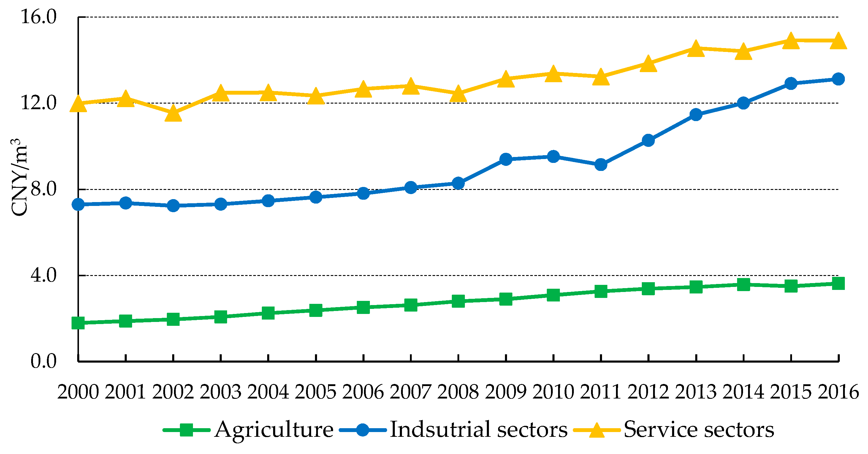
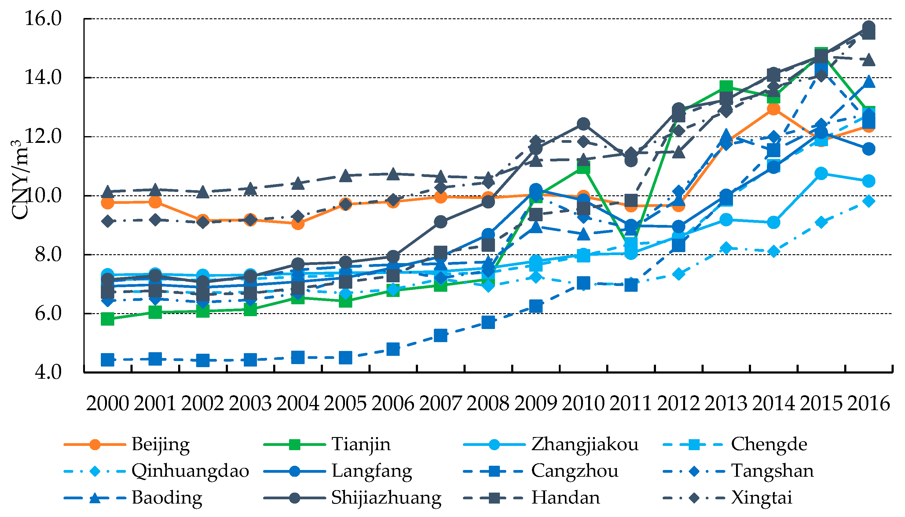
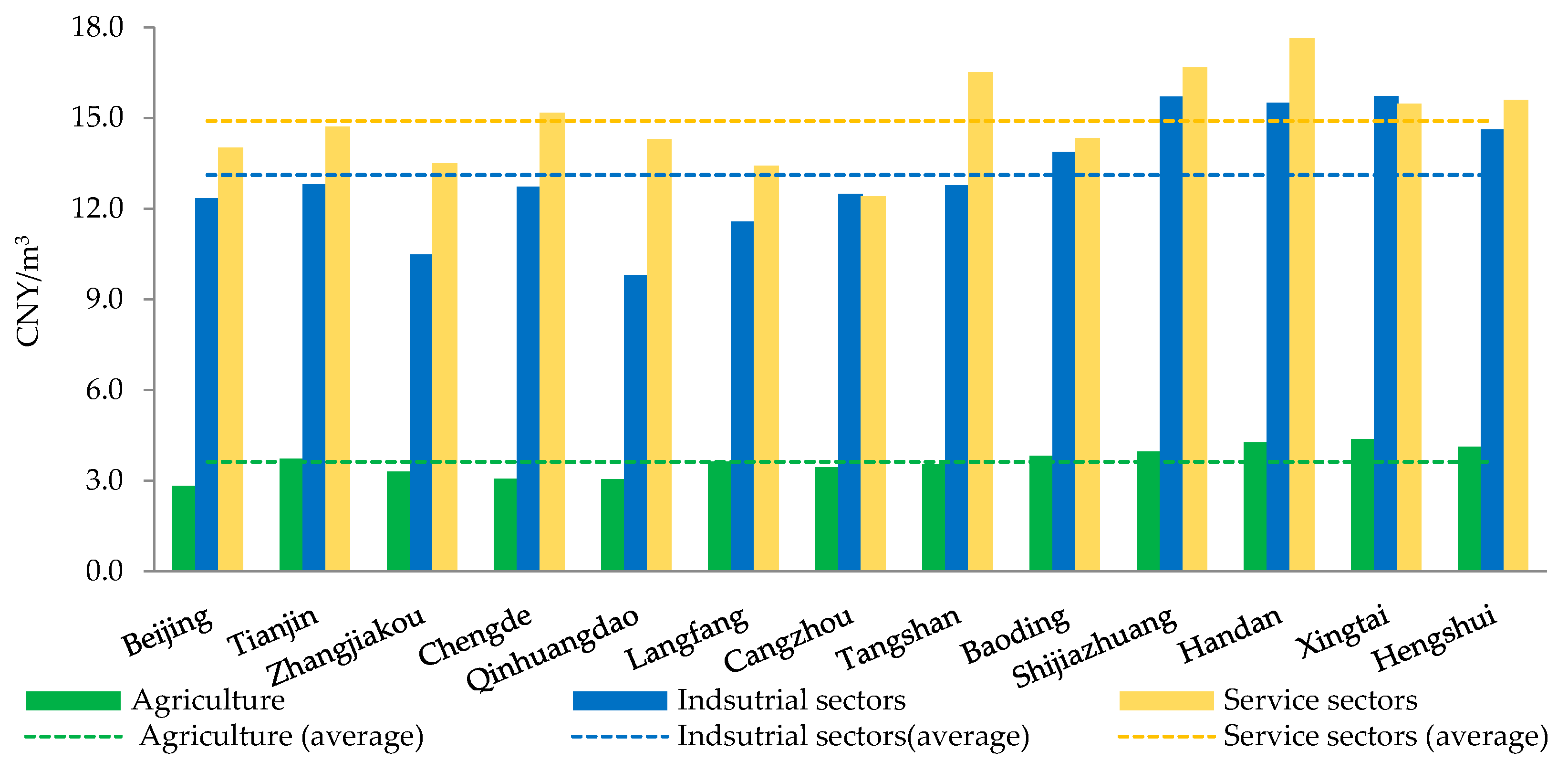
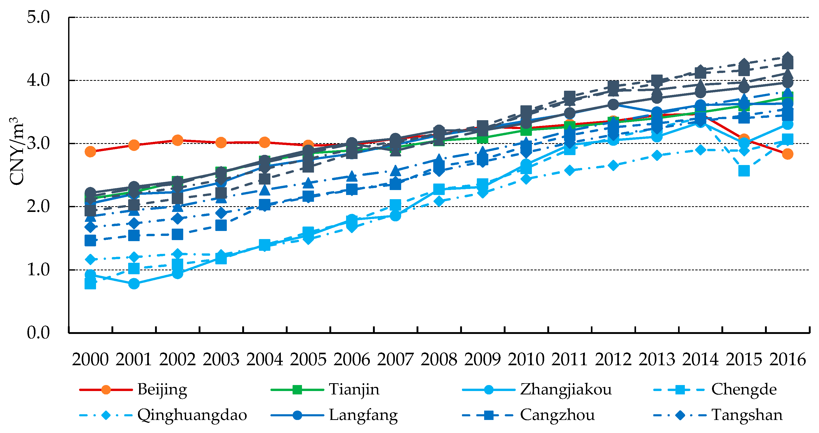
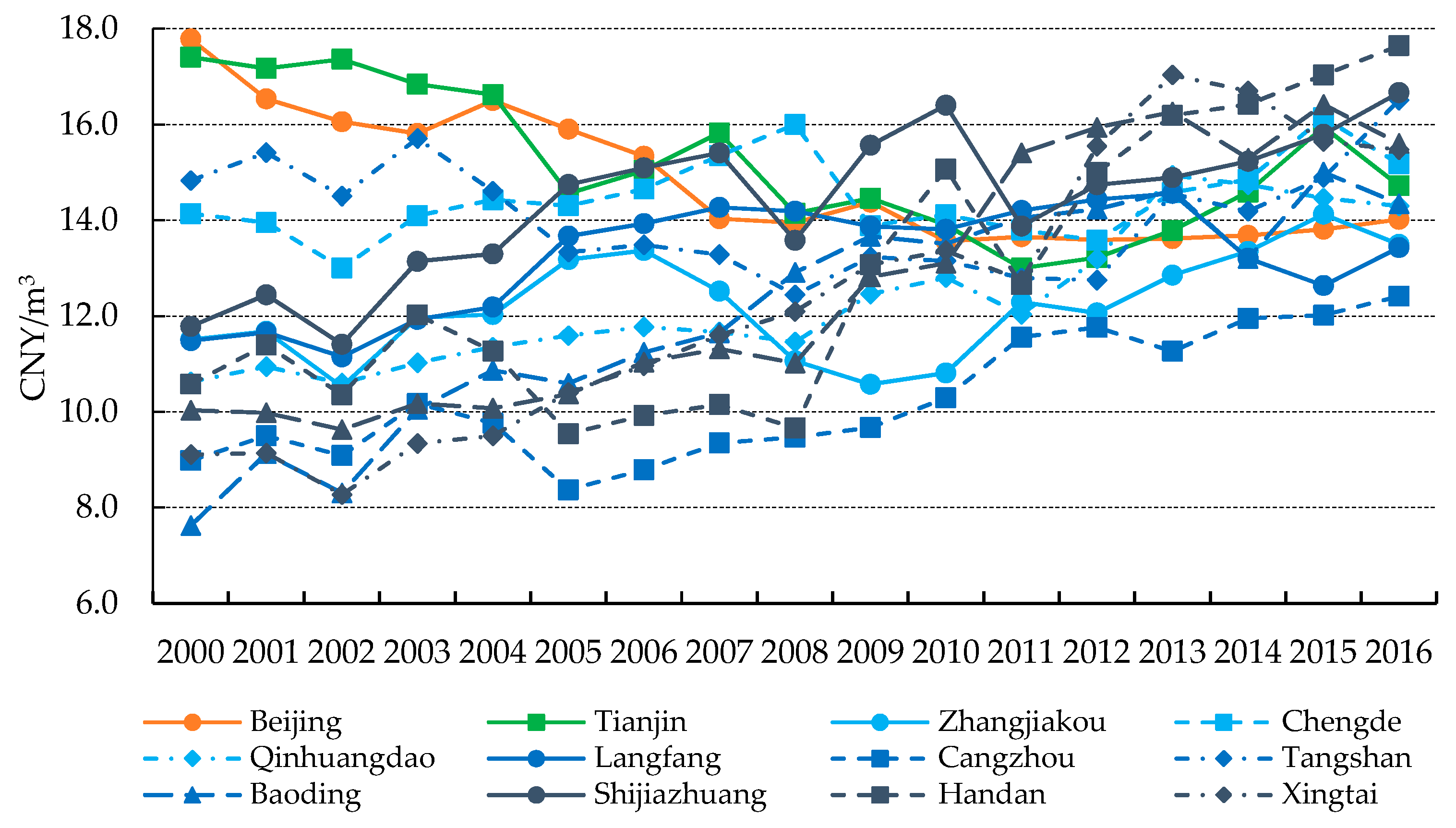
5.1. Trends of Shadow Prices of Production Water in BTH Cities

The calculation results indicate that the shadow prices of production water in Hebei continuously increase over the research period, which shows that the scarcity of production water in Hebei intensified. Meanwhile, there are significant disparities in water scarcity amongst the different parts of Hebei, being more severe in southern than in northern Hebei. Compared with the cities in Hebei, the increases in the scarcity of production water in Beijing and Tianjin are milder, while the water scarcity in their service sectors even declined.

The reasons for the regional discrepancies in water scarcity may be attributed to the following factors. First, Beijing and Tianjin have better access to more advanced technologies for water saving and more stringent environmental regulations. Although technology development has also improved the water use efficiency in Hebei, it is not sufficient to offset its huge water demand due to rapid industrialization and urbanization, let alone for the cities in southern Hebei (i.e., Hengshui and Xingtai), where water-saving measures have not been fully implemented and the relevant regulations are rather loose. Second, the water prices in Beijing and Tianjin are higher than in Hebei, which contains the expansion of its water demand to some extent. In 2016, the actual prices of industrial water in Beijing and Tianjin were 9.92 CNY/m³ and 7.85 CNY/m³ respectively, while the average industrial water price in Hebei was 5.06 CNY/m³. The difference in water pricing for the service sector is greater, especially for special industries (the industries that use water as raw material for production, mainly including bathing, car washing, etc.). Beijing’s water price for special industries is 161.68 CNY/m³, higher than Hebei’s, where the average price is 21.5 CNY/m³. Moreover, the regional discrepancy in water endowment is also relevant to the regional differences in water scarcity.

In addition, cross-sectoral water re-allocation is not considered in the optimization settings in this paper, mainly because one of the main focuses of this paper is to use the shadow price of water to indicate the current scarcity of water resources, rather than the factors affecting shadow prices. Of course, cross-sectoral water re-allocation will affect the value of shadow prices. According to the nature of the shadow price, if a certain degree of cross-sector water redistribution is allowed, just as in Nechifor’s research [7], the shadow price of the sector with reduced water resources will increase (in this paper, the agricultural sector), while the shadow price of the sector with increased water resources will decrease (the industrial and service sectors). The extent of shadow price changes is determined by the production process and the scarcity of water resources in each sector.

As the shadow price of water has been studied for a long time, our results can be compared with those of extant studies. Compared with Liu’s research [21], the shadow price of water is marginally higher, which may be due to the differences between calculation models and survey time. Further, compared with Shen [23] and Wang’s research [24], the shadow price of agricultural water in Tianjin is lower, and that of industrial water in Tianjin and Hebei is higher in this paper, which may be mainly due to the differences in the production function form and sample data level.

5.2. Water Scarcity is Underestimated in the BTH City Region

Water shadow prices theoretically reflect the real value and degree of water scarcity without administrative influences. Here, the ratio of shadow prices to actual prices (STA) is used to measure the deviation between actual and shadow price. STAs higher than 1 refer to the shadow price exceeding the actual price, meaning water scarcity is underestimated. The higher the STAs are than 1, the higher the degree of underestimation.

The STAs of the industrial sector in the BTH city region are all above 1 and reveal an uptrend during 2007–2016, which indicates an increasing degree of underestimation. The STAs of industrial water use in the cities of southern Hebei are generally higher than in other sub-regions or cities. Compared with cities in Hebei, The STAs of the industry sectors in Beijing and Tianjin are lower (

Table 6. The ratio of shadow prices to actual prices (STA) of industrial sectors in the BTH city region (2007–2016).

Regions	Cities	2007	2008	2009	2010	2011	2012	2013	2014	2015	2016
Beijing		1.8	1.8	1.8	1.6	1.6	1.6	1.9	1.5	1.2	1.2
Tianjin		0.9	1.0	1.5	1.5	1.1	1.6	1.7	1.7	1.9	1.6
Northern Hebei	Zhangjiakou	1.8	1.8	1.9	2.0	2.0	2.1	2.2	2.2	2.6	2.6
	Chengde	1.3	1.3	1.4	1.4	1.5	1.5	1.8	2.0	2.1	2.3
	Qinhuangdao	2.3	2.2	2.3	1.2	1.2	1.2	1.4	1.3	1.5	1.6
	Average	1.7	1.7	1.8	1.5	1.5	1.6	1.7	1.8	2.0	2.1
Central Hebei	Langfang	1.6	1.7	2.0	1.9	1.8	1.8	2.0	2.1	2.4	2.3
	Cangzhou	1.1	1.2	1.3	1.1	1.1	1.3	1.6	1.8	2.3	2.0
	Tangshan	2.1	2.2	2.2	1.6	1.5	1.7	2.0	2.1	2.1	2.2
	Baoding	3.5	2.3	2.1	2.0	2.1	2.3	2.8	2.7	2.9	3.3
	Average	1.8	1.8	1.9	1.6	1.6	1.7	2.0	2.1	2.4	2.4
Southern Hebei	Shijiazhuang	2.5	2.4	2.6	2.8	2.5	2.9	2.9	3.1	3.3	3.6
	Handan	1.7	1.8	2.0	2.0	2.0	2.6	2.8	3.0	3.1	3.4
	Xingtai	3.3	3.4	3.7	2.0	2.0	2.1	2.2	2.4	2.4	2.7
	Hengshui	4.3	3.1	3.3	3.3	3.4	3.4	3.9	4.0	4.3	4.3
	Average	2.7	2.6	2.8	2.4	2.4	2.7	2.9	3.0	3.2	3.4
Regional average		1.9	1.9	2.0	1.8	1.7	1.9	2.1	2.2	2.3	2.3

Note: The water price data of industrial sectors in the BTH city region is collected from the website of www.h2o-china.com/price/ [63].

). The STAs of service sectors in the BTH city region have been generally stable during 2007–2016, indicating the degree of underestimation of water scarcity remained at a stable level in each city. The STAs of service sectors in Beijing and Tianjin are in general not higher than 2, being lower than those in the cities of Hebei. The STAs in southern Hebei are still the highest, some even exceeding 3 (

Table 7. The ratio of shadow prices to actual prices (STA) of service sectors in the BTH city region (2007–2016).

Regions	Cities	2007	2008	2009	2010	2011	2012	2013	2014	2015	2016
Beijing		1.9	1.8	2.0	1.7	1.7	1.7	1.6	1.0	0.9	0.9
Tianjin		2.1	1.9	2.1	1.8	1.7	1.6	1.7	1.8	2.0	1.8
Northern Hebei	Zhangjiakou	2.5	2.2	2.2	2.2	2.5	2.5	2.6	2.7	2.9	2.7
	Chengde	2.1	2.2	1.9	1.9	1.9	1.9	2.0	2.0	2.2	2.0
	Qinhuangdao	2.3	2.3	2.4	2.0	1.9	2.1	2.3	2.3	2.3	2.2
	Average	2.3	2.2	2.1	2.0	2.0	2.1	2.3	2.3	2.4	2.3
Central Hebei	Langfang	1.7	1.8	1.7	1.7	1.8	1.8	1.8	1.6	1.6	1.7
	Cangzhou	1.3	1.2	1.3	1.6	1.8	1.9	1.8	1.9	1.9	1.9
	Tangshan	2.5	2.3	2.4	2.2	2.2	2.2	2.5	2.4	2.5	2.8
	Baoding	3.3	1.4	3.1	3.1	3.2	3.3	3.4	3.1	3.5	3.3
	Average	2.1	1.6	2.0	2.1	2.1	2.2	2.2	2.1	2.2	2.3
Southern Hebei	Shijiazhuang	3.3	2.8	2.8	3.0	2.5	2.7	2.7	2.7	2.8	3.0
	Handan	1.7	1.7	2.2	3.0	2.5	3.0	3.2	3.3	3.4	3.5
	Xingtai	2.3	2.4	2.5	2.3	2.2	2.6	2.9	2.6	2.4	2.4
	Hengshui	2.1	1.5	1.8	1.8	2.1	2.2	2.2	1.8	2.0	1.9
	Average	2.3	2.0	2.3	2.4	2.3	2.6	2.7	2.5	2.6	2.6
Regional average		2.2	1.9	2.1	2.1	2.1	2.2	2.3	2.1	2.1	2.1

Note: The water price data of service sectors in the BTH city region is collected from the website of http://price.h2o-china.com/ [63].

).

It is worth nothing that a pricing mechanism for agricultural water has not been fully implemented in the BTH city region yet. The current agricultural water pricing is determined based on non-volumetric charges, such as fees paid for electricity consumption. The current agricultural water price in the BTH city region is around 0.3–0.4 CNY/m³, merely 10% of the shadow price. This means the scarcity of water for agriculture is mostly underestimated by current agricultural water price.

Recently, the BTH city region has recognized the seriousness of its water shortage problem, implementing strict water price adjustment and issuing their “Opinions on the most stringent water resources management system” in 2016, according to the “Notice of the General Office of the State Council on Implementing the Most Strict Water Resources Management System Assessment Measures.” Each city also regards water use and water intensity as strict hard-test indicators of the “National Economic and Social Development Plan.” These measures will certainly encourage water users to increase their awareness of water conservation, improve water efficiency, and minimize the economic losses caused by water resources.

5.3. Agricultural Water Saving in Hebei is Key to Solving Water Scarcity in the BTH City Region

The results of this study indicate that water scarcity has a significant restrictive impact on the urban economic growth of the BTH city region, with Hebei bearing the largest economic loss due to this water scarcity. Hebei is one of the most important grain production bases in China, supporting the entire nation with large amounts of grain and vegetables, with high water consumption and low added value every year; the majority of production water use is attributed to agricultural water use, the proportion of which in total production water was 78.3% in 2017 [64]. For example, southern Hebei is the main area for growing winter wheat, the irrigation for which has been proven to be closely related to the overexploitation of groundwater [65]. Therefore, agricultural water saving in Hebei is key to solving the problem of water scarcity in the entire BTH city region.

Currently, most cities of Hebei still adopt traditional and backward irrigation methods. The utilization efficiency of irrigation water is very low, and the waste of water resources is very serious. The utilization rate of water-saving projects is not high. Although the irrigation area of water-saving projects is increasing year by year, the management and maintenance of water-saving equipment in rural areas are not in place due to technical management, with many water-saving projects being idle and the utilization rate not high.

Facing an aggravating water crisis, the best way for Hebei to reduce agricultural water use and the associated potential economic loss is to further improve irrigation water use efficiency. Further, improved agronomic measures, such as soil water management, irrigation system innovation, and water-saving technology applications, can effectively increase irrigation water use efficiency, and thus ensure agricultural production using less water.

Moreover, the results indicate that the pricing mechanism for agricultural water in Hebei fails to reflect the degree of water scarcity, causing the scarcity of agricultural water use in Hebei to be substantially underestimated. Low water prices will, thus, lead to wasting water resources, increasing water scarcity, and ultimately affecting economic development. To enhance Hebei’s transformation of water management from a traditionally extensive pattern to an intensive one, a rational pricing mechanism for agricultural water use that properly reflects water scarcity is urgently needed. The agricultural water price should not only be increased but also differentiated based on crop types (i.e., food or cash crops). It is noteworthy that repricing agricultural water use can increase agricultural input costs, where the trade-off between the water conservation effects and the increasing costs needs to be considered and an appropriate balance sought.

In addition to reducing agricultural water use, there are other ways to alleviate water shortages in the BTH city region. As such, the government and the market must cooperate. On one hand, water resources are distributed through government administrative means to ensure the integrity and healthy operation of the industrial system; on the other hand, the establishment of a water rights market allows water resources to be redistributed according to their economic contributions, maximizing the value of water resources while ensuring a national base. Coastal cities (Tianjin, Cangzhou, Tangshan, Qinhuangdao) can use seawater desalination technology to expand the utilization of seawater resources and enable the abstraction of drinking water from the mouths of great rivers, which would be led by a pipeline below the water level and would follow the route of the seacoast [6]; the South-to-North Water Transfer Project can also provide water from the Yangtze River to alleviate water shortages in the study area.

6. Conclusions

This study measures the water scarcity of the 13 cities in the BTH city region and the restrictive impacts of water scarcity on urban economic growth based on an optimization analysis. The main findings are:

(1) Water scarcity in the BTH city region, reflected by the water shadow price, shows significant sectoral and regional heterogeneities. At the sectoral level, the shadow price of agricultural water use is the lowest, while that of service water use is the highest. At the regional level, southern Hebei faces the most severe water scarcity in the BTH city region. Moreover, water is becoming increasingly scarce in most sectors and cities in the BTH city region, especially in southern Hebei, the region with the most severe water scarcity. While water scarcity in Beijing has improved to some extent in the agriculture and service sectors in recent years, there is still a long way to go in solving this problem.

(2) The shadow price of production water is much higher than its actual price in the BTH city region, indicating that the scarcity of water use in the region is significantly underestimated. The scarcity of industrial and service water in southern Hebei is mostly underestimated. Further, the scarcity of agriculture water use in the BTH city region is mostly underestimated, since the current agricultural water pricing is determined based on non-volumetric changes, and it is merely 10% of the shadow price.

(3) Water scarcity has a negative impact and total economic loss of CNY 270.02 billion for the BTH city region. The economic loss caused by water scarcity in Hebei is largest, especially in southern Hebei, whose potential GDP decreased by 6.2%. At the sectoral level, the potential economic losses caused by water scarcity in the industrial and service sectors are far higher than in agriculture. Moreover, the potential economic losses of the three major industries in Hebei are higher than those in Beijing and Tianjin.

However, this study only provides a preliminary analysis of the potential economic loss associated with water scarcity. To deepen the understanding, a quantitative analysis of the mechanism of how water scarcity impacts urban development is needed, which would be conducive to more effective and pertinent evidence for policy making.

References

1. Xie, Y.L.; Xia, D.X.; Ji, L.; Huang, G.H. An inexact stochastic-fuzzy optimization model for agricultural water allocation and land resources utilization management under considering effective rainfall. Ecol. Indic. 2018, 92, 301–311. [Google Scholar] [CrossRef]
2. Fan, Y.R.; Huang, W.W.; Li, Y.P.; Huang, G.H.; Huang, K. A coupled ensemble filtering and probabilistic collocation approach for uncertainty quantification of hydrological models. J. Hydrol. 2015, 530, 255–272. [Google Scholar] [CrossRef]
3. Abdulbaki, D.; Al-Hindi, M.; Yassine, A.; Abou Najm, M. An optimization model for the allocation of water resources. J. Clean. Prod. 2017, 164, 994–1006. [Google Scholar] [CrossRef]
4. Yu, S.; Lu, H. An integrated model of water resources optimization allocation based on projection pursuit model—Grey wolf optimization method in a transboundary river basin. J. Hydrol. 2018, 559, 156–165. [Google Scholar] [CrossRef]
5. Wikipedia Contributors. World Water Assessment Programme; Wikipedia: 2019. Available online: http://www.unesco.org/new/en/natural-sciences/environment/water/wwap/ (accessed on 15 January 2019).
6. Albiero, D.; Silva, M.D.D.; Melo, R.; Garcia, A.P.; Praciano, A.C.; Fernandes, F.B.; Monteiro, L.D.A.; Chioderoli, C.; Silva, A.O.D.; Filho, J.D.B. Economic Feasibility of Underwater Adduction of Rivers for Metropolises in Semiarid Coastal Environments: Case Studies. Water 2018, 10, 215. [Google Scholar] [CrossRef]
7. Nechifor, V.; Winning, M. Global Economic and Food Security Impacts of Demand-Driven Water Scarcity—Alternative Water Management Options for a Thirsty World. Water 2018, 10, 1442. [Google Scholar] [CrossRef]
8. Roson, R.; Damania, R. The macroeconomic impact of future water scarcity: An assessment of alternative scenarios. J. Policy Model. 2017, 39, 1141–1162. [Google Scholar] [CrossRef]
9. National Bureau of Statistics of China. China Statistical Yearbook 2018; China Statistical Press: Beijing, China, 2018.
10. Wang, Y.; Bian, Y.; Xu, H. Water use efficiency and related pollutants’ abatement costs of regional industrial systems in China: A slacks-based measure approach. J. Clean. Prod. 2015, 101, 301–310. [Google Scholar] [CrossRef]
11. Zeng, Z.; Liu, J.G.; Savenije, H.H.G. A simple approach to assess water scarcity integrating water quantity and quality. Ecol. Indic. 2013, 34, 441–449. [Google Scholar] [CrossRef]
12. Liu, J.; Liu, Q.; Yang, H. Assessing water scarcity by simultaneously considering environmental flow requirements, water quantity, and water quality. Ecol. Indic. 2016, 60, 434–441. [Google Scholar] [CrossRef]
13. Brown, A.; Marty, D.M. A Review of Water Scarcity Indices and Methodologies. 2011, pp. 1–21. Available online: http://www.sustainabilityconsortium.org/wp-content/themes/sustainability./pdf/whitepapers/ 2011_Brown_Matlock_Water-Availability-Assessment-Indices-and-Methodologies-Lit-Review.pdf (accessed on 7 October 2012).
14. Pedro-Monzonís, M.; Solera, A.; Ferrer, J.; Estrela, T.; Paredes-Arquiola, J. A review of water scarcity and drought indexes in water resources planning and management. J. Hydrol. 2015, 527, 482–493. [Google Scholar] [CrossRef]
15. Kummu, M.; Ward, P.J.; de Moel, H.; Varis, O. Is physical water scarcity a new phenomenon? Global assessment of water shortage over the last two millennia. Environ. Res. Lett. 2010, 5, 034006. [Google Scholar] [CrossRef]
16. Hoekstra, A.Y.; Mekonnen, M.M.; Chapagain, A.K.; Mathews, R.E.; Richter, B.D. Global monthly water scarcity: Blue water footprints versus blue water availability. PLoS ONE 2012, 7, e32688. [Google Scholar] [CrossRef]
17. Gain, A.K.; Giupponi, C. A dynamic assessment of water scarcity risk in the Lower Brahmaputra River Basin: An integrated approach. Ecol. Indic. 2015, 48, 120–131. [Google Scholar] [CrossRef]
18. Zhao, J.; Ni, H.; Peng, X.; Li, J.; Chen, G.; Liu, J. Impact of water price reform on water conservation and economic growth in China. Econ. Anal. Policy 2016, 51, 90–103. [Google Scholar] [CrossRef]
19. Wang, D.; Wang, H.; Yin, M. Implication of water resources and its value. Adv. Water Sci. 1999, 10, 195–200. [Google Scholar]
20. Houk, E.E.; Taylor, G.; Frasier, W.M. Valuing the Characteristics of Irrigation Water in the Platte River Basin. Western Agricultural Economics Association Annual Meetings. Vancouver, BC, Canada, 2000. [Google Scholar]
21. Eshghi, F. Determining the shadow price of water using MGA method: A case study of Dasht Naz of Sari-Iran. Afr. J. Agric. Res. 2012, 7, 1800–1804. [Google Scholar]
22. Liu, X.; Chen, X. Methods for Approximating the Shadow Price of Water in China. Econ. Syst. Res. 2008, 20, 173–185. [Google Scholar] [CrossRef]
23. Huang, Q.Q.; Rozelle, S.; Howitt, R.; Wang, J.X.; Huang, J.K. Irrigation water demand and implications for water pricing policy in rural China. Environ. Dev. Econ. 2010, 15, 293–319. [Google Scholar] [CrossRef]
24. Shen, X.; Lin, B. The shadow prices and demand elasticities of agricultural water in China: A StoNED-based analysis. Resour. Conserv. Recycl. 2017, 127, 21–28. [Google Scholar] [CrossRef]
25. Wang, W.; Xie, H.; Zhang, N.; Xiang, D. Sustainable water use and water shadow price in China’s urban industry. Resour. Conserv. Recycl. 2018, 128, 489–498. [Google Scholar] [CrossRef]
26. Zhang, X.; Xu, Q.; Zhang, F.; Guo, Z.; Rao, R. Exploring shadow prices of carbon emissions at provincial levels in China. Ecol. Indic. 2014, 46, 407–414. [Google Scholar] [CrossRef]
27. Wang, K.; Che, L.; Ma, C.; Wei, Y.-M. The shadow price of CO2 emissions in China’s iron and steel industry. Sci. Total Environ. 2017, 598, 272–281. [Google Scholar] [CrossRef]
28. Tang, K.; Gong, C.; Wang, D. Reduction potential, shadow prices, and pollution costs of agricultural pollutants in China. Sci. Total Environ. 2016, 541, 42–50. [Google Scholar] [CrossRef]
29. Färe, R.; Grosskopf, S.; Weber, W.L. Shadow prices and pollution costs in U.S. agriculture. Ecol. Econ. 2006, 56, 89–103. [Google Scholar] [CrossRef]
30. Van Ha, N.; Kant, S.; Maclaren, V. Shadow prices of environmental outputs and production efficiency of household-level paper recycling units in Vietnam. Ecol. Econ. 2008, 65, 98–110. [Google Scholar] [CrossRef]
31. Liu, W.D.; Lu, D.D. The effect of water resources shortage on regional economic development. Sci. Geogr. Sin. 1993, 1, 9–16. [Google Scholar]
32. Romer, D. Advanced Macroeconomics, 5th ed.; McGraw-Hill: New York, NY, USA, 2019; pp. 137–141. [Google Scholar]
33. Hua, J.; Wang, D. Research on relationship between agricultural water and agricultural economy based on growth drag of water resources. Acta Agric. Jiangxi 2018, 30, 129–133. [Google Scholar]
34. Wang, X.Y.; Han, H.Y. Growth drag of water resources to agriculture in China. J. Econ. Water Resour. 2008, 3, 1–5. [Google Scholar]
35. Zhang, H.Q.; Zhang, C.J.; Zhang, W.L. Water resource constraints and China’s economic growth—Based on econometric analysis of “Resistance” of water resource. Ind. Econ. Res. 2016, 4, 87–99. [Google Scholar]
36. Berrittella, M.; Hoekstra, A.Y.; Rehdanz, K.; Roson, R.; Tol, R.S.J. The economic impact of restricted water supply: A computable general equilibrium analysis. Water Res. 2007, 41, 1799–1813. [Google Scholar] [CrossRef] [PubMed]
37. Zang, C.; Liu, J.; Jiang, L.; Gerten, D. Impacts of human activities and climate variability on green and blue water flows in the Heihe River Basin in Northwest China. Hydrol. Earth Syst. Sci. 2013, 10, 9477–9504. [Google Scholar] [CrossRef]
38. Kosolapova, N.A.; Matveeva, L.G.; Nikitaeva, A.Y.; Molapisi, L. Modeling resource basis for social and economic development strategies: Water resource case. J. Hydrol. 2017, 553, 438–446. [Google Scholar] [CrossRef]
39. Leroux, A.D.; Martin, V.L.; Zheng, H. Addressing water shortages by force of habit. Resour. Energy Econ. 2018, 53, 42–61. [Google Scholar] [CrossRef]
40. Qin, C.; Su, Z.; Bressers, H.T.A.; Jia, Y.; Wang, H. Assessing the economic impact of North China’s water scarcity mitigation strategy: A multi-region, water-extended computable general equilibrium analysis. Water Int. 2013, 38, 701–723. [Google Scholar] [CrossRef]
41. Maestre-Valero, J.F.; Martínez-Granados, D.; Martínez-Alvarez, V.; Calatrava, J. Socio-Economic Impact of Evaporation Losses from Reservoirs Under Past, Current and Future Water Availability Scenarios in the Semi-Arid Segura Basin. Water Resour. Manag. 2013, 27, 1411–1426. [Google Scholar] [CrossRef]
42. Bruvoll, A.; Glomsrød, S.; Vennemo, H. Environmental drag: Evidence from Norway. Ecol. Econ. 1999, 30, 235–249. [Google Scholar] [CrossRef]
43. Li, N.; Wang, X.; Shi, M.; Hong, Y. Economic Impacts of Total Water Use Control in the Heihe River Basin in Northwestern China—An Integrated CGE-BEM Modeling Approach. Sustainability 2015, 7, 3460–3478. [Google Scholar] [CrossRef]
44. Distefano, T.; Kelly, S. Are we in deep water? Water scarcity and its limits to economic growth. Ecol. Econ. 2017, 142, 130–147. [Google Scholar] [CrossRef]
45. Zhou, Q.; Deng, X.; Wu, F. Impacts of water scarcity on socio-economic development: A case study of Gaotai County, China. Phys. Chem. Earth Parts A/B/C 2017, 101, 204–213. [Google Scholar] [CrossRef]
46. National Bureau of Statistics of China. China Statistical Yearbook 2007; China Statistical Press: Beijing, China, 2007.
47. Beijing Water Resources Bulletin. 2000–2016. Available online: http://www.bjwater.gov.cn/bjwater/ (accessed on 10 October 2018).
48. Tianjin Water Resources Bulletin. 2000–2016. Available online: http://swj.tj.gov.cn/pub/tjwcb/index.html (accessed on 10 October 2018).
49. Hebei Province Water Resources Bulletin. 2000–2016. Available online: http://www.hebwater.gov.cn/ (accessed on 10 October 2018).
50. Hebei Economic Yearbook. 2001 to 2017. Available online: http://www.hetj.gov.cn/hetj/tjsj/jjnj/ (accessed on 9 November 2018).
51. Lei, H.; Pan, X. The calculation on the capital stock in different industries of China and the comparison of investment efficiency. J. Shanghai Univ. Int. Bus. Econ. 2016, 6, 40–52. [Google Scholar]
52. Tian, Y. Estimation on capital stock of sectors in China: 1990–2014. J. Quant. Tech. Econ. 2016, 33, 3–21. [Google Scholar]
53. Weng, H.; Wang, B. Estimation on capital stock of sectors in China. Stat. Decis. 2012, 12, 89–92. [Google Scholar]
54. Beijing Statistical Yearbook. 2001 to 2017. Available online: http://www.bjstats.gov.cn/tjsj/ (accessed on 9 November 2018).
55. Tianjin Statistical Yearbook. 2001 to 2017. Available online: http://stats.tj.gov.cn/Category_29/Index.aspx (accessed on 9 November 2018).
56. Beijing Input-Output Table. 2012. Available online: http://www.bjstats.gov.cn/ (accessed on 15 November 2016).
57. Tianjin Input-Output Table. 2012. Available online: http://stats.tj.gov.cn/Item/26895.aspx (accessed on 15 November 2016).
58. Input-Output Table of Prefectural-Level City of Hebei Province. 2012. Available online: http://www.hetj.gov.cn/hetj/tjsj/jjnj/ (accessed on 23 November 2016).
59. Färe, R.; Martins-Filho, C.; Vardanyan, M. On functional form representation of multi-output production technologies. J. Product. Anal. 2010, 33, 81–96. [Google Scholar] [CrossRef]
60. Aigner, D.J.; Chu, S.F. On Estimating the Industry Production Function. Am. Econ. Rev. 1968, 58, 826–839. [Google Scholar]
61. Leontief, W.W. Quantitative input and output relations in the economic systems of the United States. Rev. Econ. Stat. 1936, 18, 105–125. [Google Scholar]
62. Tang, Z.; Liu, W.; Fu, C.W. Optimization modeling and evolution analysis of Beijing’s industrial structure under energy constraints. Resour. Sci. 2012, 34, 29–34. [Google Scholar]
63. The water price of industrial and service sectors in the BTH. 2012. Available online: http://price.h2o-china.com/ (accessed on 15 November 2016).
64. Hebei Water Resources Bulletin. 2017. Available online: http://www.hebwater.gov.cn/ (accessed on 9 November 2018).
65. Ma, L. Comprehensive management for groundwater over-exploitation in Hebei Province. China Water Resour. 2017, 51–54. [Google Scholar]
66. Wu, J. TFP growth and convergence across China’s industrial economy considering environmental protection. J. Quant. Tech. Econ. 2009, 26, 17–27. [Google Scholar]
Figure 1. The administrative areas of the BTH city region and its economic and water resources conditions.
Sustainability 11 02452 g001
Figure 2. The average shadow prices of the production water use in the three industries in the BTH region (2000–2016).
Sustainability 11 02452 g002
Figure 3. Shadow prices of production water use in the cities of the BTH city region (2016).
Sustainability 11 02452 g003
Figure 4. The shadow price of agricultural water use in the BTH city region (2000–2016).
Sustainability 11 02452 g004
Figure 5. The shadow price of industrial water use in the BTH city region (2000–2016).
Sustainability 11 02452 g005
Figure 6. The shadow price of services water use in the BTH city region (2000–2016).
Sustainability 11 02452 g006