An Empirical Study on the Comprehensive Optimization Method of a Train Diagram of the China High Speed Railway Express


Abstract
1. Introduction
2. Literature Review
2.1. Theory and Method of Train Diagram Compilation
2.1.1. Compiling a Periodic Train Diagram Model
2.1.2. Non-Periodic Train Diagram Model
2.2. Cargo Flow Assignment Problem
2.3. Research on the Application of EMU
3. Construction of Comprehensive Optimizing Model for a High-Speed Railway Express Train Diagram
3.1. Problem Description
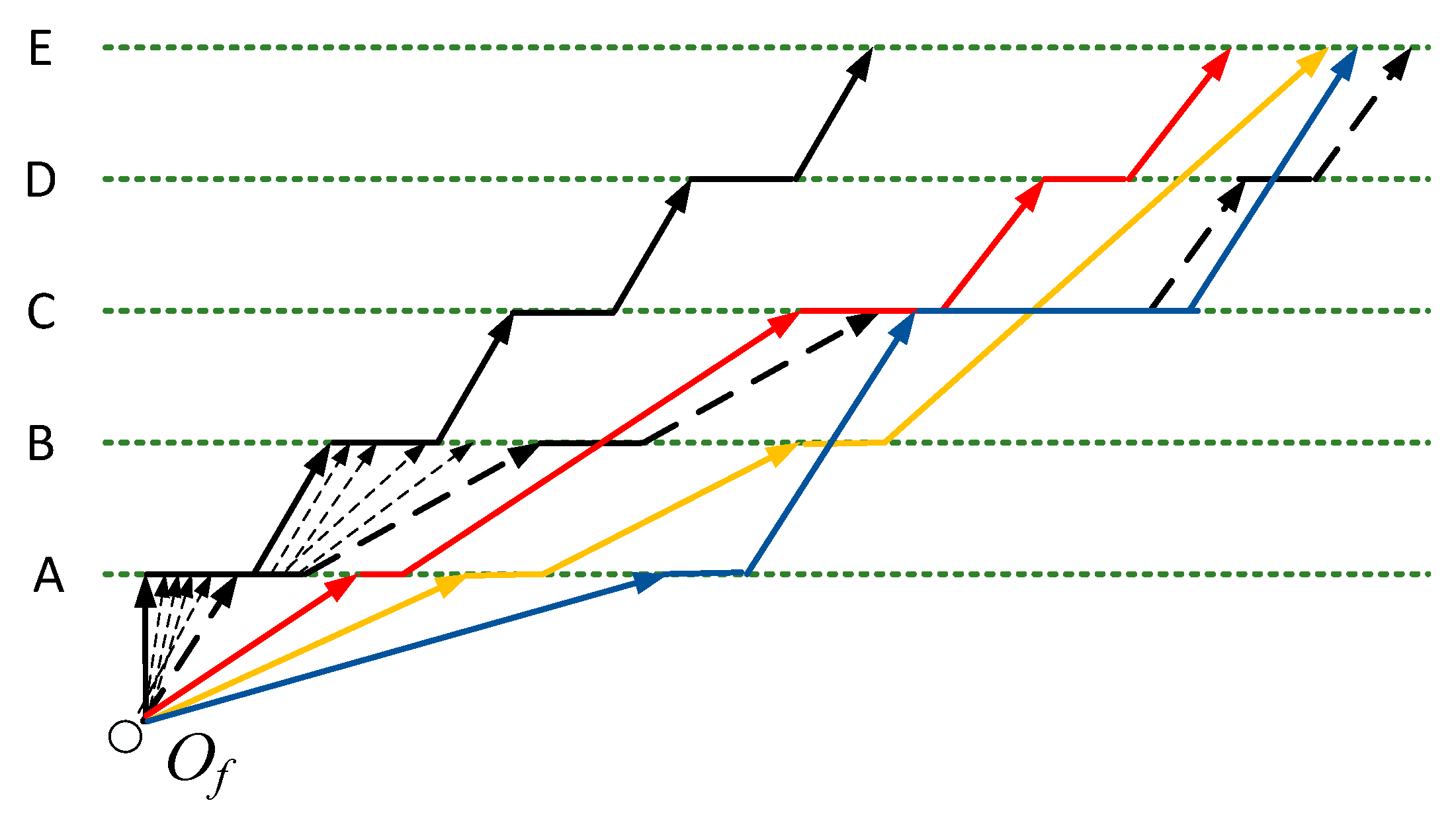
3.1.1. Compilation of High-Speed Railway Express Train Diagram: Freight Train Spatial-Temporal Service Network
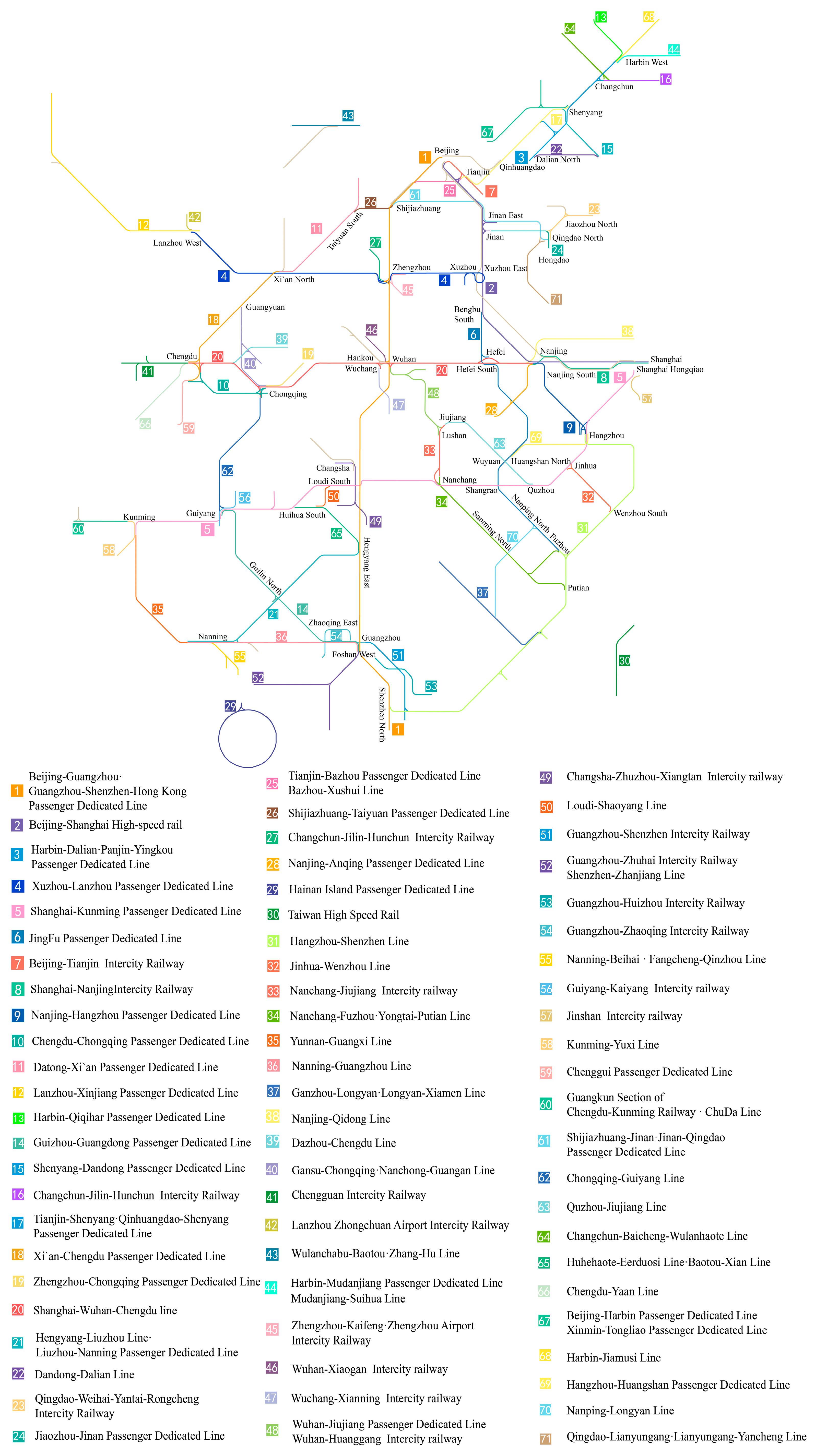
3.1.2. Distribution of Freight Flow in High-Speed Railway Express Transportation: Physical Transportation Network of a High-Speed Railway
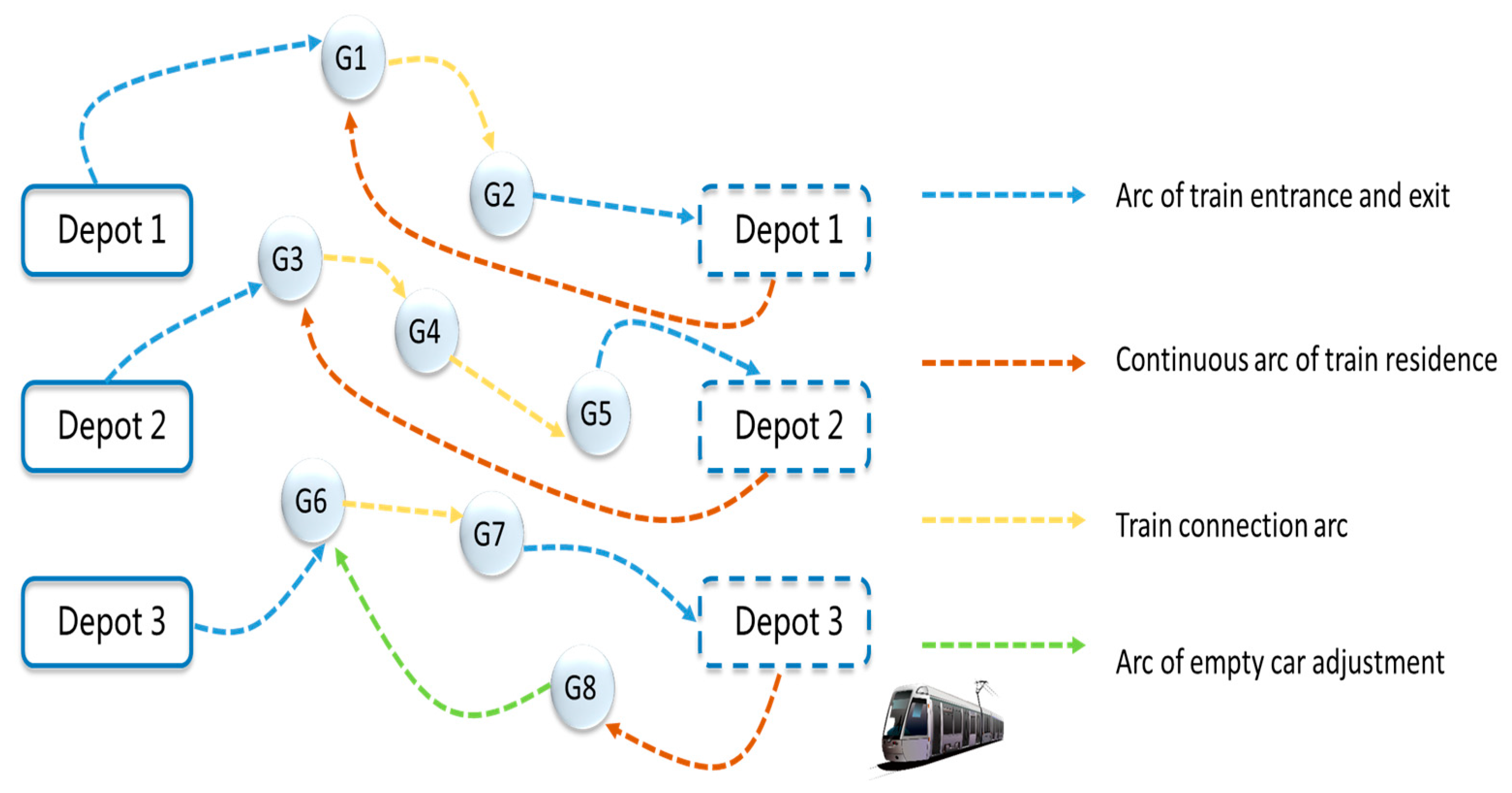
3.1.3. Operation Planning of Freight EMU-Train Connection Network
3.2. Model Hypothesis
3.2.1. Dual-Line Operation
3.2.2. Maintenance Assumptions
3.2.3. Train Operation Hypothesis
3.3. Notation
3.3.1. Sets
3.3.2. Parameters
3.3.3. Decision Variables
3.4. Model Formulation
3.4.1. Objective Function
3.4.2. Constraint Condition
- (a)
- Assignment constraints of freight trains’ spatial-temporal paths:Formula (12) indicates that for any given freight train, there is only one Spatial-temporal path to ensure the uniqueness of the same spatial-temporal path.
- (b)
- The node operating capacity constraints:Formula (13) indicates that the loading and unloading capacity of the train operation station is constrained, and the station is influenced by the track structure. It is necessary to arrange the loading and unloading operation plan reasonably to meet the loading and unloading operation requirements of all trains and to avoid conflict with passenger trains.
- (c)
- The mapping constraints of auxiliary variables:Formulas (14) and (15) denote the constraints of the mapping relationship of auxiliary variables, i.e., the decision variable is changed to 0–1 variable, which denotes the relationship between train spatial-temporal path and traffic; that is, if a certain spatial-temporal path is selected, there must be traffic, and vice versa. Formula (16) denotes the relationship between auxiliary variables and train spatial-temporal path; that is, whether a train’s spatial-temporal path is selected is related to whether the transport arc is selected in each section.
- (d)
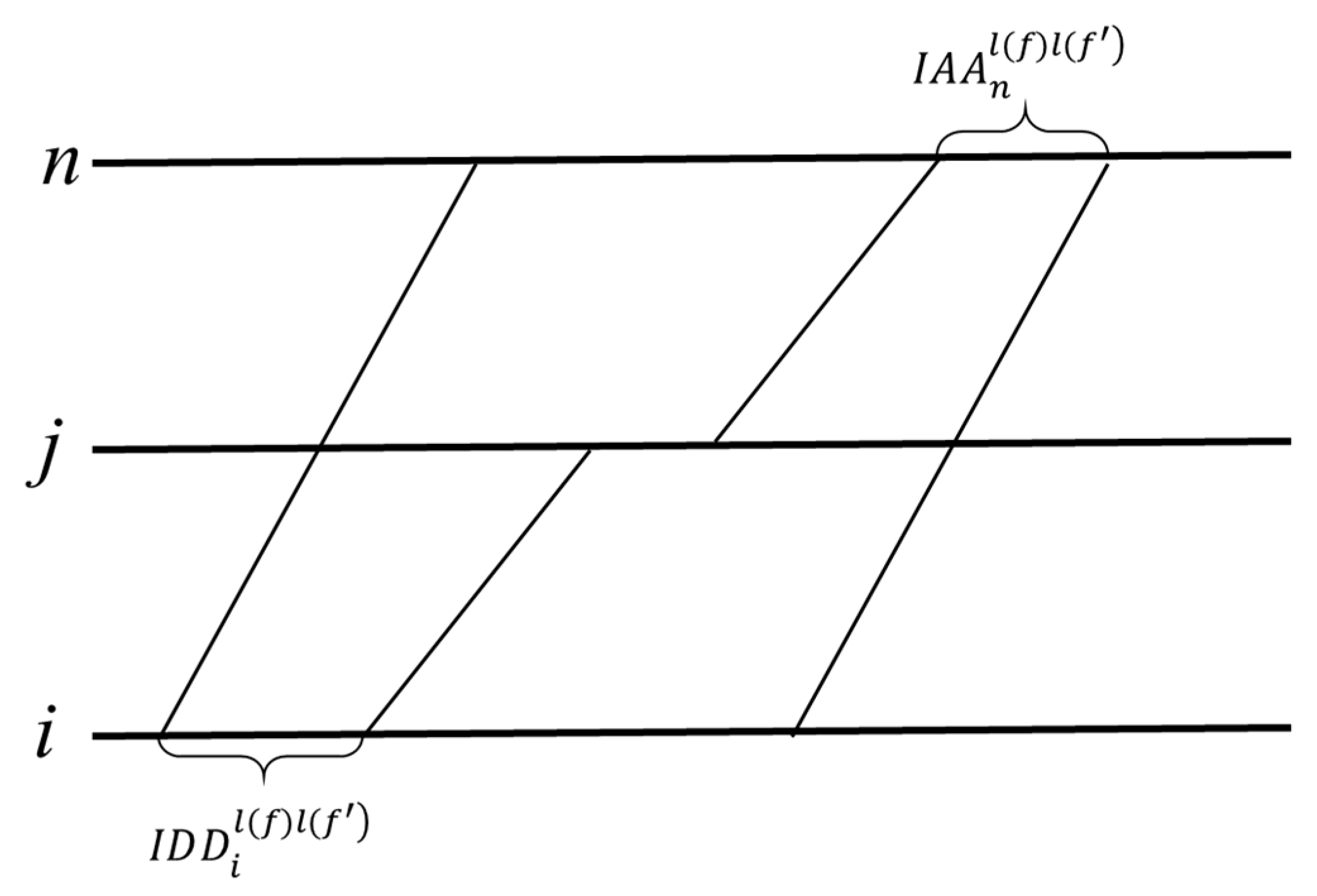
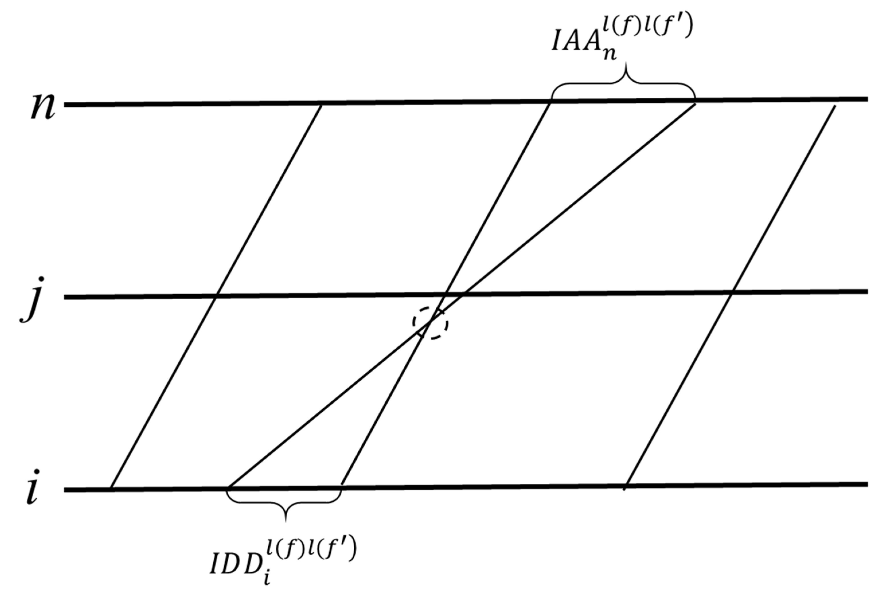
- The constraints of train safety interval time.In order to ensure traffic safety and make the most effective use of the passing capacity of the section, the train should abide by the relevant regulations and technical operation time standards of the station, and meet the constraints of safe departure and arrival time intervals. The relationship between them is shown in Figure 4.(d1) Safe departure interval constraint:(d2) Safe arrival interval constraint:In order to ensure the safety of the train in the departure throat area of the station, the minimum train tracking time is set. Formulas (17) and (18) represent the constraints of the continuous train departure interval. Formulas (19) and (20) indicate that the train must meet the constraints of the minimum arrival tracking interval.(d3) Train relationship constraints.In order to describe the relationship between trains reasonably, the constraint of prohibiting overtaking should also be considered, as shown in Figure 5.From Figure 5, it can be seen that although the train guarantees the minimum safe interval between arrival and departure, the two trains in interval show unreasonable overtaking due to the different speed grades. Therefore, in order to avoid the occurrence of such an unreasonable situation, it is necessary to define the relationship between the two trains; that is, within the interval, no overtaking can occur.Formula (21) denotes the running relationship of trains; that is, the relationship between train and remains unchanged from beginning to end, so as to ensure that and do not cross each other.
- (e)
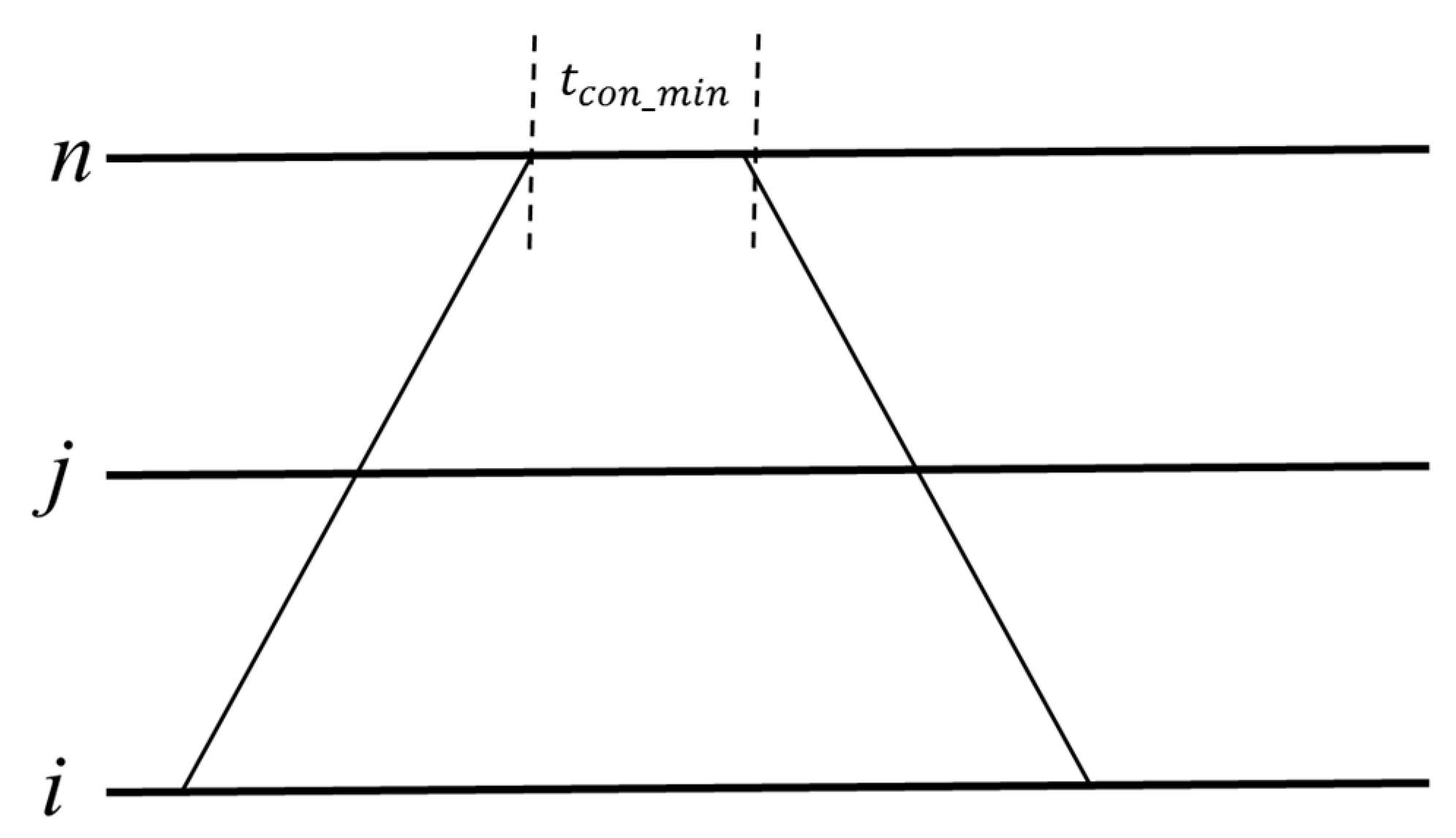
- Train connection time constraints.The train connection relationship is coupled; that is, the arrival and departure sequence and the connection time between the two trains are interrelated. The connection time between the two trains should meet the technical operation time of the nodes, as shown in Figure 6.Formula (22) indicates that the difference between the train departure time and the train arrival time should satisfy the minimum connecting time.
- (f)
- Time window constraints for freight products.At present, there are clear arrival time requirements for today’s, next morning’s, next day’s, and third day’s high-speed rail express products. Therefore, different kinds of transport products should meet different time window constraints.Formula (23) indicates that the arrival time of the goods is earlier than the latest arrival time of the transport product.
- (g)
- Flow balance constraints:Formula (24) denotes flow equilibrium constraints, i.e., for two adjacent intervals, the inflow volume equals the outflow volume. Formulas (25) and (26) indicate that the requirements of the initial node and the end-to-end node are equal to the amount of traffic sent or that has arrived, respectively.
- (h)
- Train Loading Capacity Constraints:Formula (27) expresses the constraint of full-load rate of trains. It is necessary to run freight trains only when the freight flow reaches a certain amount, so as to ensure economic benefits.Form (28) denotes the capacity constraints of passenger or freight trains. The total amount of goods loaded by trains should not exceed the maximum carrying capacity of trains.
- (i)
- Routing constraints of freight EMUs:Formula (29) means that a given freight train task must be undertaken by a certain freight train set; that is, all tasks need to be performed by the EMU. Formula (30) means that the operation of the train cannot exceed the maintenance capacity of the EMU depot. Formula (31) means that all freight train sets cannot exceed the given number of EMUs.
- (j)
- Range Constraints of Decision Variables:Formulas (32)–(34) denotes the range constraints of decision variables.
4. Algorithm Design
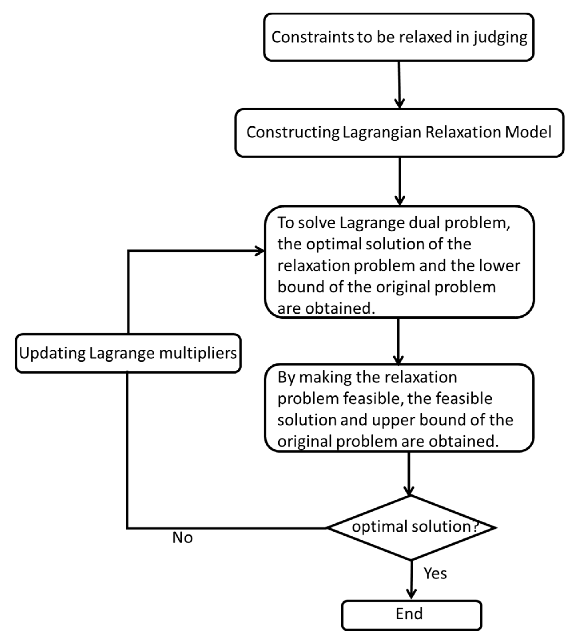
4.1. Algorithm Principle and Low
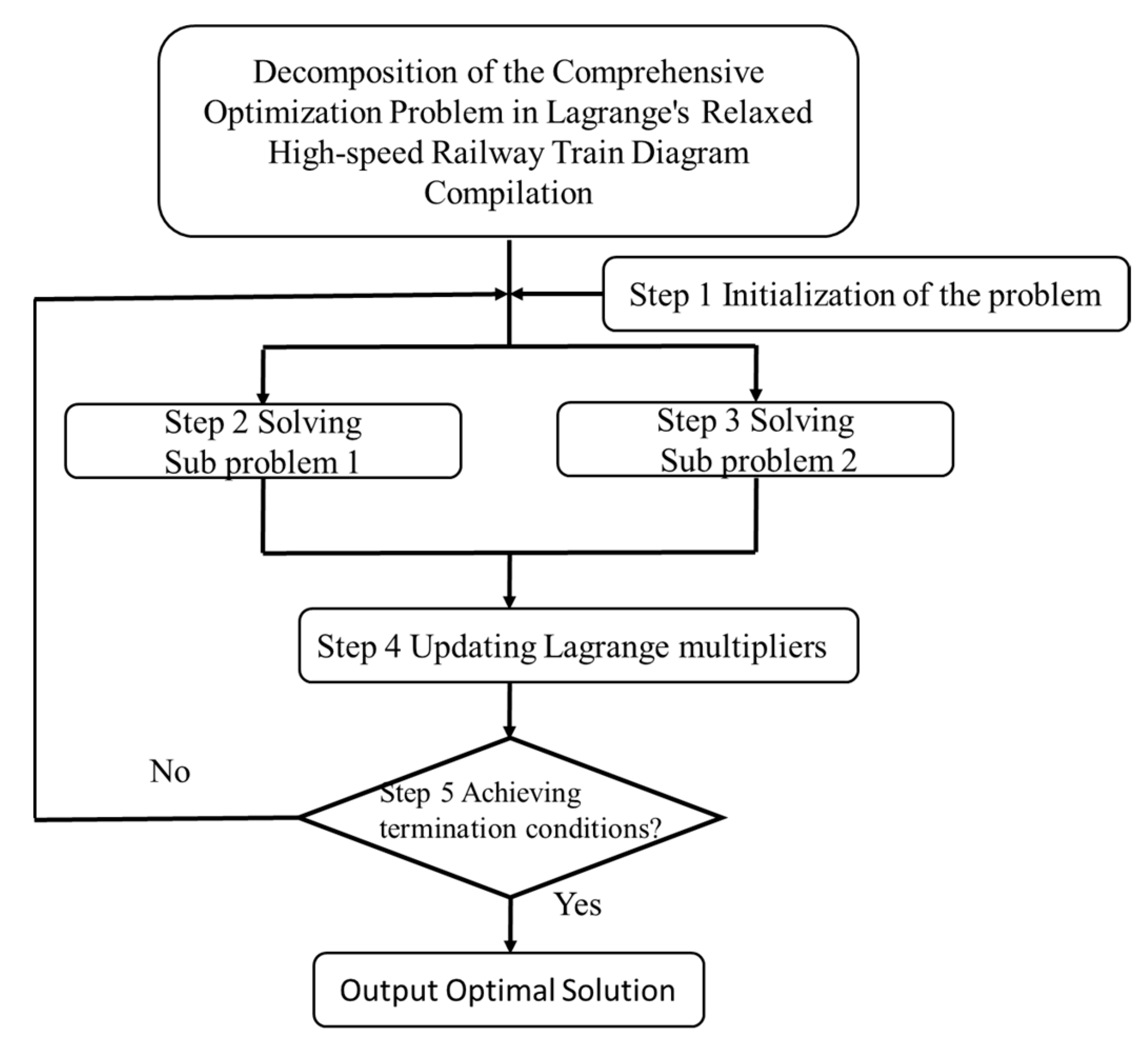
4.2. Algorithm Steps
- Step 1:
- Problem InitializationSet the number of iterations ;Initialization of Lagrange multipliers;Initial sub-gradient iteration step size .
- Step 2:
- Solving Sub-problem 1The dynamic programming algorithm is used to search the shortest path with additional constraints.
- Step 3:
- Solving Sub-problem 2The dynamic programming algorithm is used to search the shortest path with resource constraints.
- Step 4:
- Updating Lagrange multipliers with the sub-gradient optimization process① Computing Lagrange multipliers:② Updating Lagrange multipliers:
- Step 5:
- Closing condition
4.3. The Solution and Computation of Sub Problems
4.3.1. Solution of Sub Problem 1
| Algorithm 1 Dynamic programming labeling method: |
| Input: Spatio-temporal network , Starting point , Terminal point , Resource cost vector, Initial value of Lagrange multiplier. Output: Minimum cost path from start to terminal . Step 1: Parameter initialization Create an empty list of node collections , set , , Insert into the collection list . Step 2: Update the node label When is a nonempty set do Remove a node from For node do If Then The cost of setting a new label alternate node is: End If If Then The labeling cost of the recording node is Record as the precursor node of End If // Updating the cost label of the node End For Delete node from End do Step 3: Get the shortest spatio-temporal path Step 3.1 Find the minimum cost node corresponding to the end point, and set as the current node Step 3.2 Nodes backtracking to While Current node is not (1) Find the precursor of the current node (2) Update the current node as the current node End Step 3.3 Output Minimum Cost Path Step 3.4 Algorithm termination |
4.3.2. Solution of Sub Problem 2
| Algorithm 2. dynamic programming algorithm. |
| Setting the initial state: , , , , ; Set: While Select a node i from LN For all do For all do If is not empty and is better than the existing label in then Set: Delete the label eliminated by from Add to only when is not in End If End Output final label. |
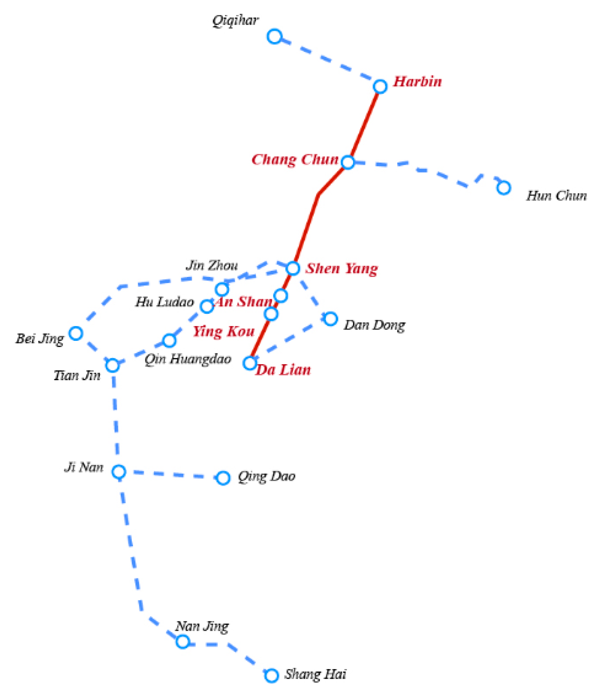
5. Case Analysis
5.1. Parameter Value
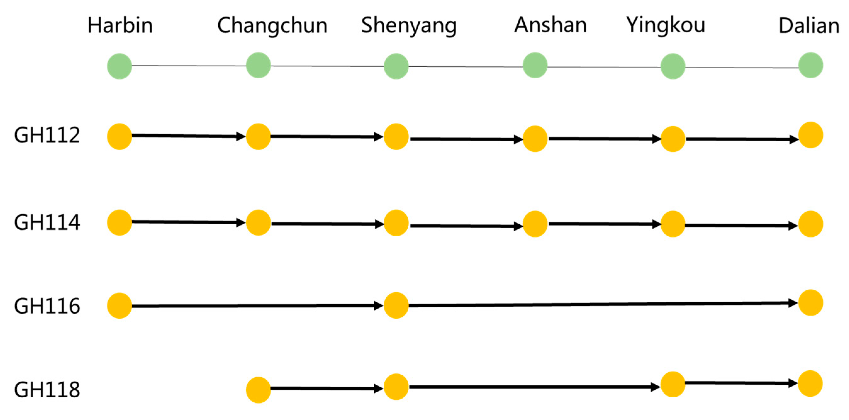
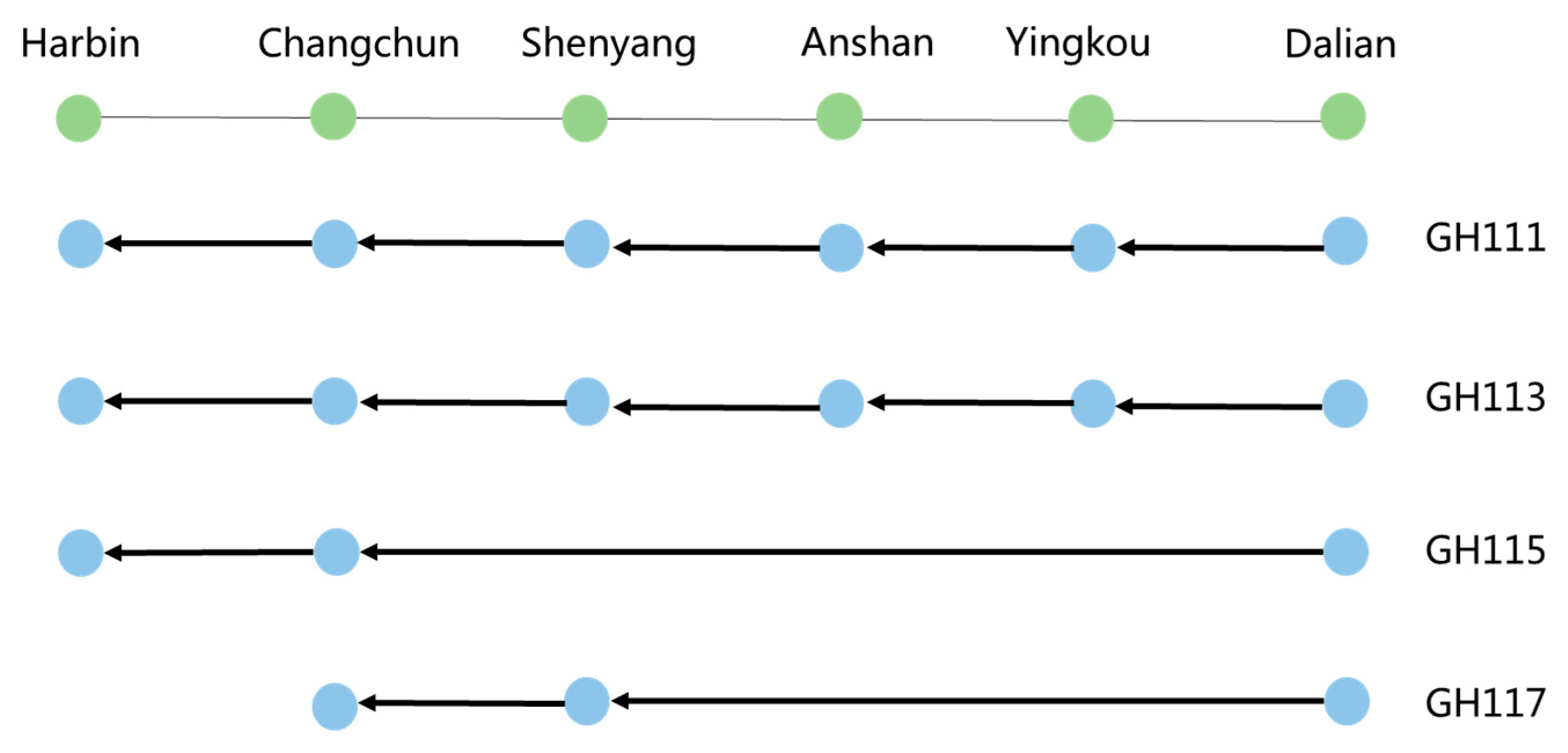
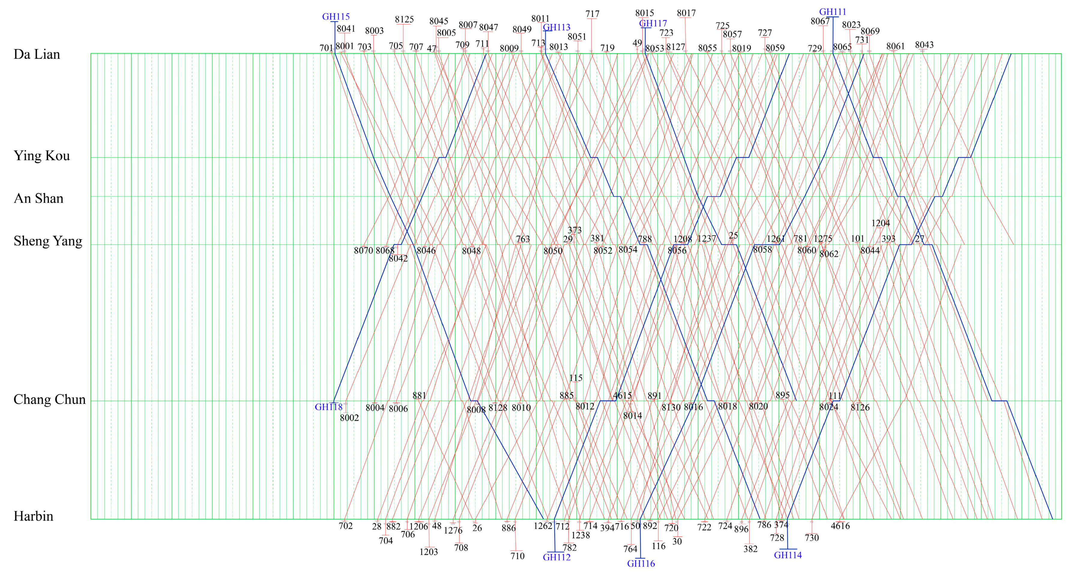
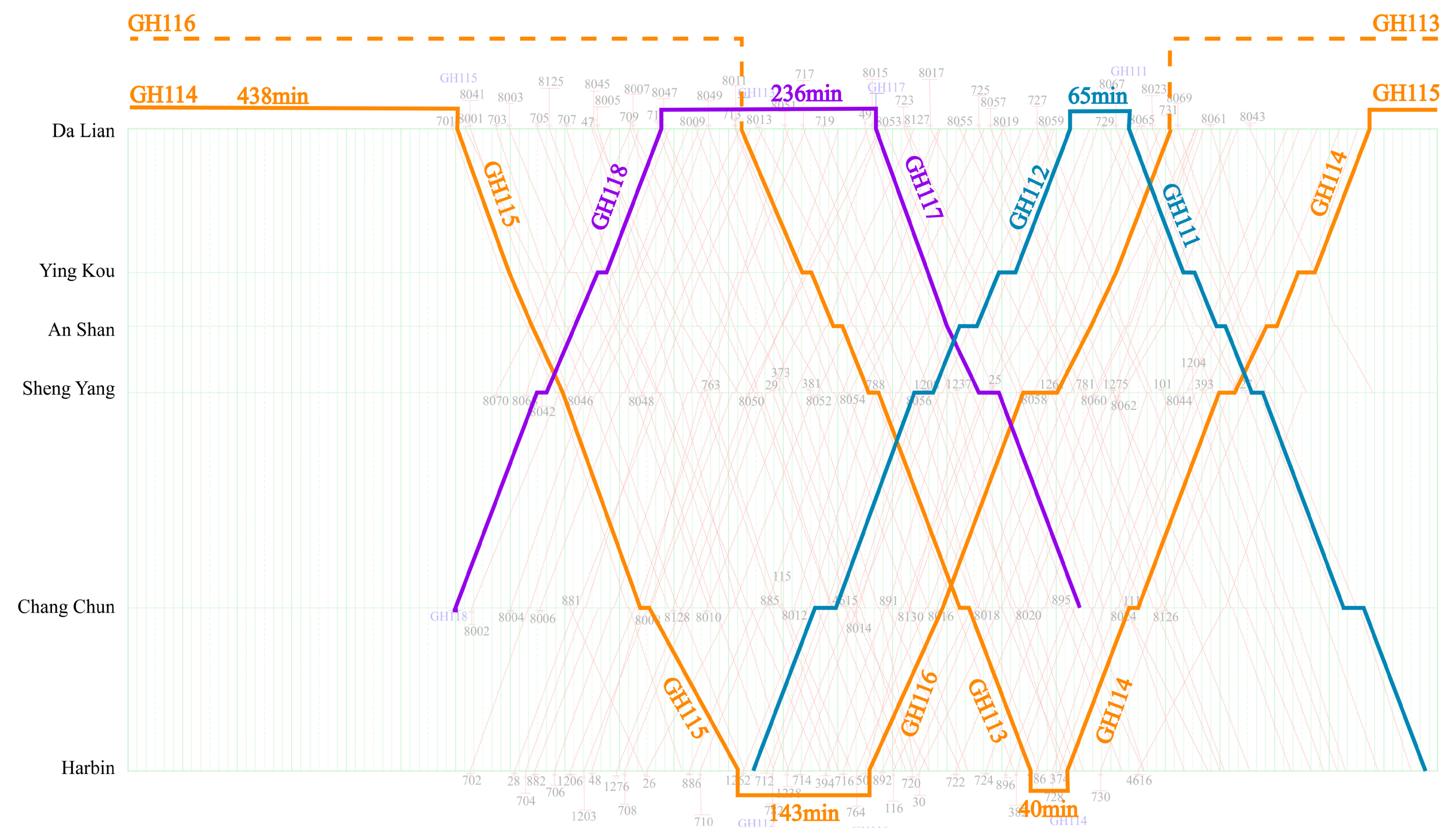
5.2. High-Speed Railway Express Train Diagram
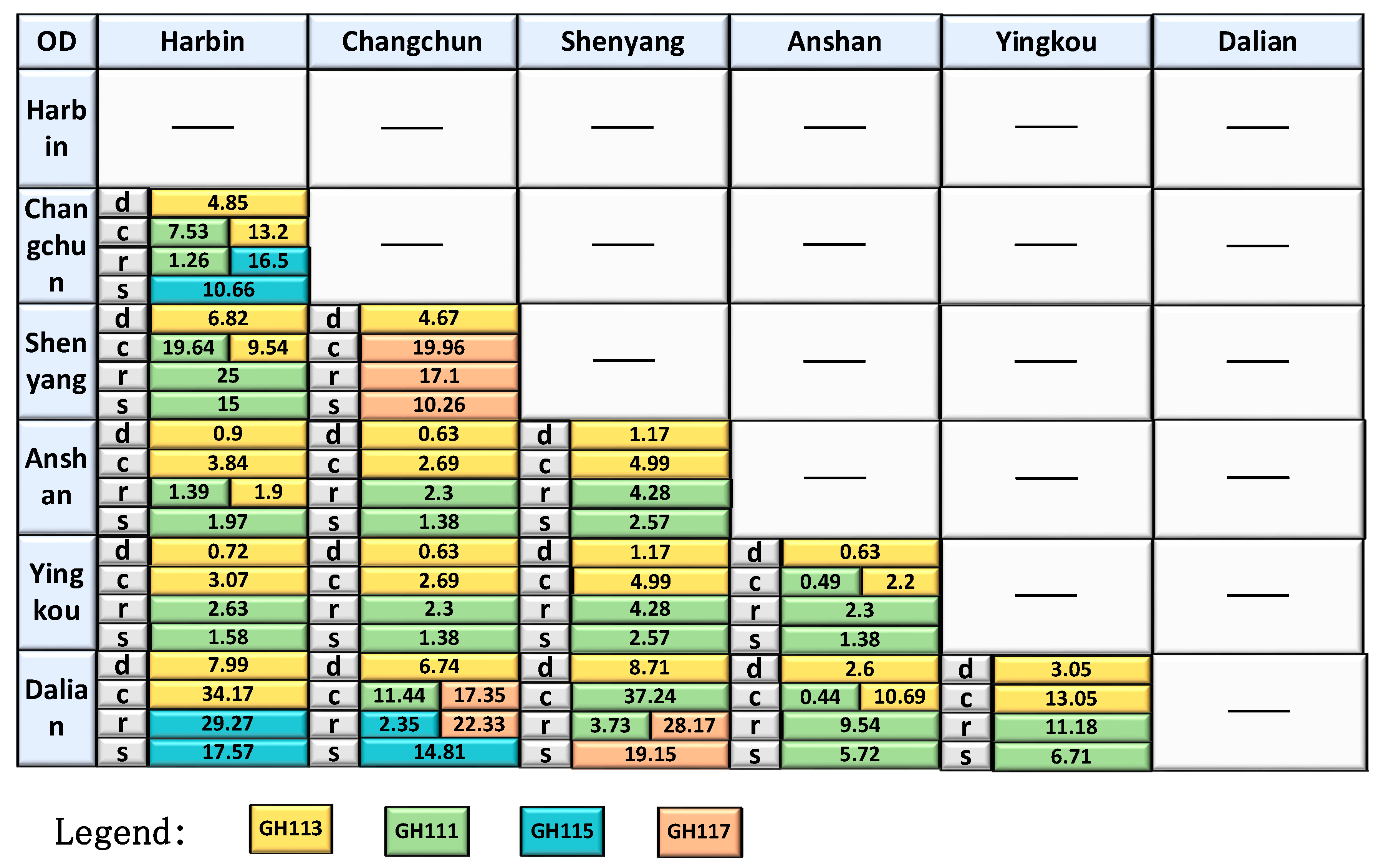
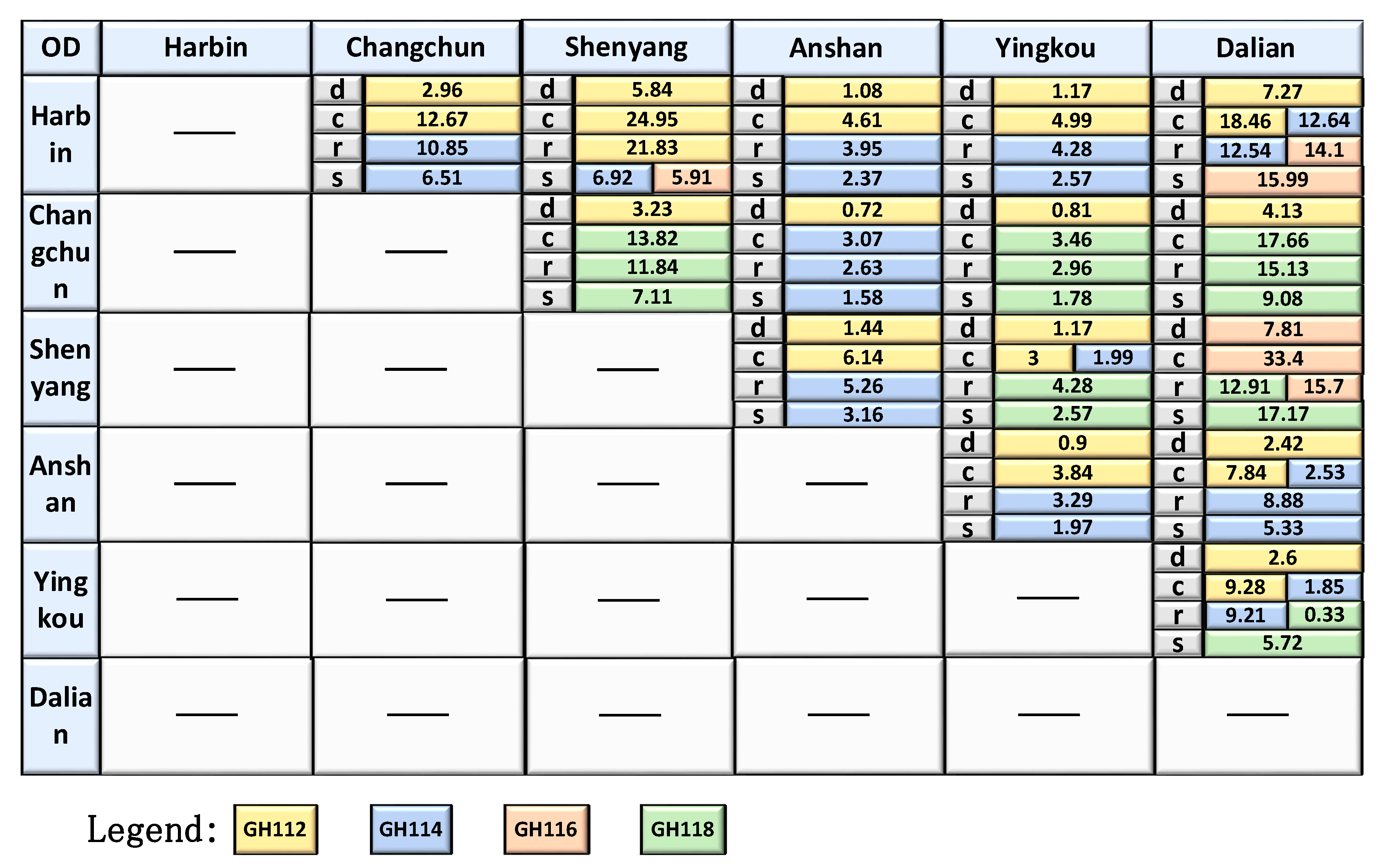
5.3. Flow Distribution Scheme for High-Speed Railway Express Trains
6. Conclusions
Author Contributions
Funding
Conflicts of Interest
References
- Chen, Y.; Whalley, A. Green Infrastructure: The Effects of Urban Rail Transit on Air Quality. Am. Econ. J. Econ. Policy 2012, 4, 58–97. [Google Scholar] [CrossRef]
- Yu, X.; Lang, M.; Gao, Y.; Wang, K.; Su, C.-H.; Tsai, S.-B.; Huo, M.; Yu, X.; Li, S. An empirical study on the Design of China High-Speed Rail Express Train Operation Plan—From a Sustainable Transport Perspective. Sustainability 2018, 10, 2478. [Google Scholar] [CrossRef]
- Ngo, N.T.; Indraratna, B.; Rujikiatkamjorn, C. Simulation Ballasted Track Behavior: Numerical Treatment and Field Application. ASCE-Int. J. Geomech. 2017, 17, 04016130. [Google Scholar] [CrossRef]
- Sayeed, M.A.; Shahin, M.A. Three-dimensional numerical modelling of ballasted railway track foundations for high-speed trains with special reference to critical speed. Transp. Geotech. 2016, 6, 55–65. [Google Scholar] [CrossRef]
- Chen, F.; Shen, X.; Wang, Z.; Yang, Y. An Evaluation of the Low-Carbon Effects of Urban Rail Based on Mode Shifts. Sustainability 2017, 9, 401. [Google Scholar] [CrossRef]
- Carey, M. A model and strategy for train pathing with choice of lines, platforms, and routes. Transp. Res. Part B 1994, 28, 353. [Google Scholar] [CrossRef]
- Caprara, A.; Fischetti, M.; Toth, P. Modeling and Solving the Train Timetabling Problem. Oper. Res. 2002, 50, 851–861. [Google Scholar] [CrossRef]
- Serafini, P.; Ukovich, W. A Mathematical Model for Periodic Scheduling Problems. SIAM J. Discrete Math. 1989, 2, 550–581. [Google Scholar] [CrossRef]
- Kroon, L.G.; Peeters, L.W.P. A Variable Trip Time Model for Cyclic Railway Timetabling. Transp. Sci. 2003, 37, 198–212. [Google Scholar] [CrossRef]
- Yang, L.; Qi, J.; Li, S.; Gao, Y. Collaborative optimization for train scheduling and train stop planning on high-speed railways. Omega 2016, 64, 57–76. [Google Scholar] [CrossRef]
- Caimi, G.; Kroon, L.; Liebchen, C. Models for railway timetable optimization: Applicability and applications in practice. J. Rail Transp. Plan. Manag. 2016, 6, 285–312. [Google Scholar] [CrossRef]
- Caimi, G.; Fuchsberger, M.; Laumanns, M.; Kaspar, S. A multi-level framework for generating train schedules in highly utilised networks. Public Transp. 2011, 3, 3–24. [Google Scholar] [CrossRef]
- Fallah, R.; Alam, S.; Nikbakhsh, R. Relationship between Knowledge Management and Innovation in Employees of Sport Organization of Tehran Municipality. PROMET-Traffic Transp. 2014, 26, 243–255. [Google Scholar]
- Sparing, D.; Goverde RM, P. A cycle time optimization model for generating stable periodic railway timetables. Transp. Res. Part B Methodol. 2017, 98, 198–223. [Google Scholar] [CrossRef]
- Cacchiani, V.; Caprara, A.; Toth, P. A column generation approach to train timetabling on a corridor. 4OR Q. J. Oper. Res. 2008, 6, 125–142. [Google Scholar] [CrossRef]
- Zhou, X.; Zhong, M. Single-track train timetabling with guaranteed optimality: Branch-and-bound algorithms with enhanced lower bounds. Transp. Res. Part B Methodol. 2007, 41, 320–341. [Google Scholar] [CrossRef]
- Zhou, X.; Zhong, M. Bicriteria train scheduling for high-speed passenger railroad planning applications. Eur. J. Oper. Res. 2005, 167, 752–771. [Google Scholar] [CrossRef]
- Yue, Y.; Wang, S.; Zhou, L.; Tong, L.; Rapik, M. Optimizing train stopping patterns and schedules for high-speed passenger rail corridors. Transp. Res. Part C Emerg. Technol. 2016, 63, 126–146. [Google Scholar] [CrossRef]
- Cordeau, J.F.; Toth, P.; Vigo, D. A Survey of Optimization Models for Train Routing and Scheduling. Transp. Sci. 1998, 32, 380–404. [Google Scholar] [CrossRef]
- Haghani, A.E. Formulation and solution of a combined train routing and makeup, and empty car distribution model. Transp. Res. Part B Methodol. 1989, 23, 433–452. [Google Scholar] [CrossRef]
- Holmbergab, K. Lagrangian based heuristics for the multicommodity network flow problem with fixed costs on paths. Eur. J. Oper. Res. 2008, 188, 101–108. [Google Scholar] [CrossRef]
- Sun, Y.; Cao, C.; Wu, C. Multi-objective optimization of train routing problem combined with train scheduling on a high-speed railway network. Transp. Res. Part C Emerg. Technol. 2014, 44, 1–20. [Google Scholar] [CrossRef]
- Lingaya, N.; Cordeau, J.F.; Desaulniers, G.; Desrosier, J.; Soumis, F. Operational car assignment at VIA Rail Canada. Transp. Res. Part B Methodol. 2002, 36, 778. [Google Scholar] [CrossRef]
- Fioole, P.J.; Kroon, L.; Maróti, G.; Schrijver, A. A rolling stock circulation model for combining and splitting of passenger trains. Eur. J. Oper. Res. 2006, 174, 1281–1297. [Google Scholar] [CrossRef]
- Abbink, E.; Bianca, V.D.B.; Kroon, L.; Salomon, M. Allocation of Railway Rolling Stock for Passenger Trains. Transp. Sci. 2004, 38, 33–41. [Google Scholar] [CrossRef]
- Alfieri, A.; Groot, R.; Kroon, L.; Schrijver, A. Efficient Circulation of Railway Rolling Stock. Transp. Sci. 2006, 40, 378–391. [Google Scholar] [CrossRef]
- Dauzère-Pérès, S.; De Almeida, D.; Guyon, O.; Benhizia, F. A Lagrangian heuristic framework for a real-life integrated planning problem of railway transportation resources. Transp. Res. Part B Methodol. 2015, 74, 138–150. [Google Scholar] [CrossRef]
- Espinosa-Aranda, J.L.; García-Ródenas, R.; Cadarso, L.; Marín, Á. Train Scheduling and Rolling Stock Assignment in High Speed Trains. Procedia Soc. Behav. Sci. 2014, 160, 45–54. [Google Scholar] [CrossRef]
- Giacco, G.L.; Carillo, D.; D’Ariano, A.; Pacciarelli, D.; Marín, Á.G. Short-term Rail Rolling Stock Rostering and Maintenance Scheduling. Transp. Res. Procedia 2014, 3, 651–659. [Google Scholar] [CrossRef]
- Zhou, L.; Lu, T.; Chen, J.; Tang, J.; Zhou, X. Joint optimization of high-speed train timetables and speed profiles: A unified modeling approach using space-time-speed grid networks. Transp. Res. Part B Methodol. 2017, 97, 157–181. [Google Scholar] [CrossRef]
- Luan, X.; Wang, Y.; De Schutter, B.H.K.; Meng, L.; Gabriel, L.; Francesco, C. Integration of real-time traffic management and train control for rail networks—Part 2, Extensions towards energy-efficient train operations. Transp. Res. Part B Methodol. 2018, 115, 72–94. [Google Scholar] [CrossRef]


| Research object | ① Optimization of train formation and undercarriage connection ② Application of EMU in rush hour ③ Establishment of maintenance plan for EMU ④ EMU operation plan ⑤ Route Planning of EMU |
| Model characteristics | ① Integer Programming Model ② Multi-commodity flow model ③ Transition Model and Interchange Model ④ Neural Network Model |
| Objective function | ① Minimum cost of EMUs ② Optimum number and mileage of EMUs ③ Minimizing seat shortages ④ Minimizing shunting operations |
| Constraint condition | ① Flow equilibrium constraints ② Coupling constraints between operation plan and operation diagram ③ Shunting sequence constraints ④ Conservation of Number of EMUs |
| Set of stations, indexed by , where . | |
| Category set of high-speed rail express products, indexed by , where . | |
| The set of trains in the operation plan, denotes the set of passenger trains, denotes the set of freight trains, , denotes one of the trains. | |
| Spatial-temporal path set of freight trains; | |
| Route set of freight EMU. | |
| , | The set of Spatial-temporal node, , denotes the time when the train arrives and departs, where . |
| The set of the spatial-temporal arc . | |
| The set of train connection relation. | |
| The set of train pairs prohibited from overtaking. |
| Time of departure of train from station through time-space arc . | |
| Time of arrive of train from station through time-space arc . | |
| Running time cost of spatial-temporal arc . | |
| Minimum continue time for trains. | |
| Number of arrival and departure lines at station n. | |
| Interval time of train departure at station with speed grades and respectively. | |
| Interval time of train arriving at station with speed grades and , respectively. | |
| Number of freight EMUs. | |
| Daily maintenance number of freight trains. |
| The volume of train chooses spatial-temporal arc to transport product . | |
| Equals 1 if the time-space path of freight train is selected; 0 otherwise. | |
| Equals 1 if the route of freight trains is selected; 0 otherwise. | |
| Equals 1 if at the same station , the order always precedes ; 0 otherwise. | |
| Equals 1 if train f carries cargo on the Spatial-temporal path ; 0 otherwise. |
| The starting point of the train | |
| The terminal of the train | |
| Used to obtain the corresponding number of station spatio-temporal node | |
| Minimum path cost from to | |
| The spatio-temporal node of the station with minimum cost and precedence of node | |
| Cost of occupying arc | |
| Subsequent node set of node |
| Effective label set of node | |
| A label for node , for each label , represents a route from of the starting EMU depot to node | |
| Cumulative cost savings from start node to node | |
| Cumulative time from the end of last overhaul to node | |
| Accumulated train mileage from the end of last overhaul to node | |
| Boolean vectors are used to describe the visited nodes, where represents the number of trains, N represents the number of elements contained in the set, and represents the coupling relationship between EMUs and trains |
| D | Harbin | Changchun | Shenyang | Anshan | Yingkou | Dalian | |||||||||||||
|---|---|---|---|---|---|---|---|---|---|---|---|---|---|---|---|---|---|---|---|
| O | |||||||||||||||||||
| Harbin | —— | d | 2.96 | 33 | d | 5.84 | 65 | d | 1.08 | 12 | d | 1.17 | 13 | d | 7.27 | 81 | |||
| c | 12.67 | c | 24.95 | c | 4.61 | c | 4.99 | c | 31.10 | ||||||||||
| r | 10.85 | r | 21.38 | r | 3.95 | r | 4.28 | r | 26.64 | ||||||||||
| s | 6.51 | s | 12.83 | s | 2.37 | s | 2.57 | s | 15.99 | ||||||||||
| Changchun | d | 4.85 | 54 | —— | d | 3.23 | 36 | d | 0.72 | 8 | d | 0.81 | 9 | d | 4.13 | 46 | |||
| c | 20.73 | c | 13.82 | c | 3.07 | c | 3.46 | c | 17.66 | ||||||||||
| r | 17.76 | r | 11.84 | r | 2.63 | r | 2.96 | r | 15.13 | ||||||||||
| s | 10.66 | s | 7.11 | s | 1.58 | s | 1.78 | s | 9.08 | ||||||||||
| Shenyang | d | 6.82 | 76 | d | 4.67 | 52 | —— | d | 1.44 | 16 | d | 1.17 | 13 | d | 7.81 | 87 | |||
| c | 29.18 | c | 19.96 | c | 6.14 | c | 4.99 | c | 33.40 | ||||||||||
| r | 25.00 | r | 17.10 | r | 5.26 | r | 4.28 | r | 28.61 | ||||||||||
| s | 15.00 | s | 10.26 | s | 3.16 | s | 2.57 | s | 17.17 | ||||||||||
| Anshan | d | 0.90 | 10 | d | 0.63 | 7 | d | 1.17 | 13 | —— | d | 0.90 | 10 | d | 2.42 | 27 | |||
| c | 3.84 | c | 2.69 | c | 4.99 | c | 3.84 | c | 10.37 | ||||||||||
| r | 3.29 | r | 2.30 | r | 4.28 | r | 3.29 | r | 8.88 | ||||||||||
| s | 1.97 | s | 1.38 | s | 2.57 | s | 1.97 | s | 5.33 | ||||||||||
| Yingkou | d | 0.72 | 8 | d | 0.63 | 7 | d | 1.17 | 13 | d | 0.63 | 7 | —— | d | 2.60 | 29 | |||
| c | 3.07 | c | 2.69 | c | 4.99 | c | 2.69 | c | 11.13 | ||||||||||
| r | 2.63 | r | 2.30 | r | 4.28 | r | 2.30 | r | 9.54 | ||||||||||
| s | 1.58 | s | 1.38 | s | 2.57 | s | 1.38 | s | 5.72 | ||||||||||
| Dalian | d | 7.99 | 89 | d | 6.74 | 75 | d | 8.71 | 97 | d | 2.60 | 29 | d | 3.05 | 34 | —— | |||
| c | 34.17 | c | 28.79 | c | 37.24 | c | 11.13 | c | 13.05 | ||||||||||
| r | 29.27 | r | 24.67 | r | 31.90 | r | 9.54 | r | 11.18 | ||||||||||
| s | 17.57 | s | 14.81 | s | 19.15 | s | 5.72 | s | 6.71 | ||||||||||
| Harbin | Changchun | Shenyang | Anshan | Yingkou | Dalian | |
|---|---|---|---|---|---|---|
| Harbin | - | 234 | 543 | 638 | 715 | 921 |
| Changchun | 234 | - | 309 | 404 | 481 | 687 |
| Shenyang | 543 | 309 | - | 95 | 172 | 378 |
| Anshan | 638 | 404 | 95 | - | 77 | 283 |
| Yingkou | 715 | 481 | 172 | 77 | - | 206 |
| Dalian | 921 | 687 | 378 | 283 | 206 | - |
| Train Number | Station | Arrival Time | Departure Time | Operation Time (min) | Train Number | Station | Arrival Time | Departure Time | Operation Time (min) |
|---|---|---|---|---|---|---|---|---|---|
| GH111 | Dalian | ---- | 18.20 | — | GH112 | Harbin | ---- | 11.27 | — |
| Yingkou | 19.20 | 19.32 | 12 | Changchun | 12.35 | 12.58 | 23 | ||
| Anshan | 19.56 | 20.06 | 10 | Shenyang | 14.24 | 14.45 | 21 | ||
| Shenyang | 20.35 | 20.47 | 12 | Anshan | 15.14 | 15.33 | 19 | ||
| Changchun | 22.16 | 22.38 | 22 | Yingkou | 15.57 | 16.15 | 18 | ||
| Harbin | 23.46 | ---- | — | Dalian | 17.15 | ---- | — | ||
| GH113 | Dalian | ---- | 11.14 | — | GH114 | Harbin | ---- | 17.12 | — |
| Yingkou | 12.21 | 12.31 | 10 | Changchun | 18.20 | 18.30 | 10 | ||
| Anshan | 12.55 | 13.05 | 10 | Shenyang | 19.59 | 20.16 | 17 | ||
| Shenyang | 13.34 | 13.45 | 12 | Anshan | 20.51 | 21.02 | 11 | ||
| Changchun | 15.14 | 15.24 | 10 | Yingkou | 21.26 | 21.44 | 18 | ||
| Harbin | 16.32 | ---- | — | Dalian | 22.44 | ---- | — | ||
| GH115 | Dalian | ---- | 6.02 | — | GH116 | Harbin | ---- | 13.34 | — |
| Changchun | 9.23 | 9.33 | 10 | Shenyang | 16.24 | 17.01 | 37 | ||
| Harbin | 11.11 | ---- | — | Dalian | 19.06 | ---- | — | ||
| GH117 | Dalian | ---- | 13.42 | — | GH118 | Changchun | ---- | 6.00 | — |
| Shenyang | 15.35 | 15.57 | 22 | Shenyang | 7.30 | 7.40 | 10 | ||
| Changchun | 17.26 | ---- | — | Yingkou | 8.36 | 8.46 | 10 | ||
| Dalian | 9.46 | ---- | — |
© 2019 by the authors. Licensee MDPI, Basel, Switzerland. This article is an open access article distributed under the terms and conditions of the Creative Commons Attribution (CC BY) license (http://creativecommons.org/licenses/by/4.0/).
Share and Cite
Yu, X.; Lang, M.; Zhang, W.; Li, S.; Zhang, M.; Yu, X. An Empirical Study on the Comprehensive Optimization Method of a Train Diagram of the China High Speed Railway Express. Sustainability 2019, 11, 2141. https://doi.org/10.3390/su11072141
Yu X, Lang M, Zhang W, Li S, Zhang M, Yu X. An Empirical Study on the Comprehensive Optimization Method of a Train Diagram of the China High Speed Railway Express. Sustainability. 2019; 11(7):2141. https://doi.org/10.3390/su11072141
Chicago/Turabian StyleYu, Xueqiao, Maoxiang Lang, Wenhui Zhang, Shiqi Li, Mingyue Zhang, and Xiao Yu. 2019. "An Empirical Study on the Comprehensive Optimization Method of a Train Diagram of the China High Speed Railway Express" Sustainability 11, no. 7: 2141. https://doi.org/10.3390/su11072141
APA StyleYu, X., Lang, M., Zhang, W., Li, S., Zhang, M., & Yu, X. (2019). An Empirical Study on the Comprehensive Optimization Method of a Train Diagram of the China High Speed Railway Express. Sustainability, 11(7), 2141. https://doi.org/10.3390/su11072141