Article

The Impact of High-Speed Rail on the Service-Sector Agglomeration in China

1
School of Economic Management, China University of Geosciences, Wuhan 430074, China
2
School of Law and Business, Wuhan Institute of Technology, Wuhan 420205, China
*
Authors to whom correspondence should be addressed.
Sustainability 2019, 11(7), 2128; https://doi.org/10.3390/su11072128
Submission received: 5 March 2019 / Revised: 28 March 2019 / Accepted: 4 April 2019 / Published: 10 April 2019
(This article belongs to the Section Sustainable Transportation)

Abstract

:
High-speed rail (HSR) can potentially influence various economic activities across space. Estimating the impacts of HSR on service-sector agglomeration (SSA) was proven to be difficult but meaningful. In this paper, prefectural-level data from 1998 to 2016 and a panel data program evaluation method are employed to evaluate the effect of the Wuhan–Guangzhou HSR (WGHSR) on the SSA along the route. In this way, we construct hypothetical counterfactuals for SSA index of the WGHSR cities in the absence of the HSR projects using the SSA index in selected non-HSR cities. By comparing the counterfactual index and the actual index, the evaluation of the WGHSR’s impact on the SSA along the route can be obtained. The results show that: (a) the WGHSR has increased the SSA by 9.44% on average for cities along the WGHSR, and (b) the impacts of the WGHSR on the SSA are heterogeneous. The WGHSR has brought about both spillover effect and “siphon” effect. In addition, whether the HSR influences and how much it could influence the SSA requires other supplementary conditions to be met. As a national strategy in China, the construction plan of HSR should fully consider its heterogeneity of impact on regional development. Policies should be formulated to drive the HSR’s spillover effect to promote regional sustainable development.

1. Introduction

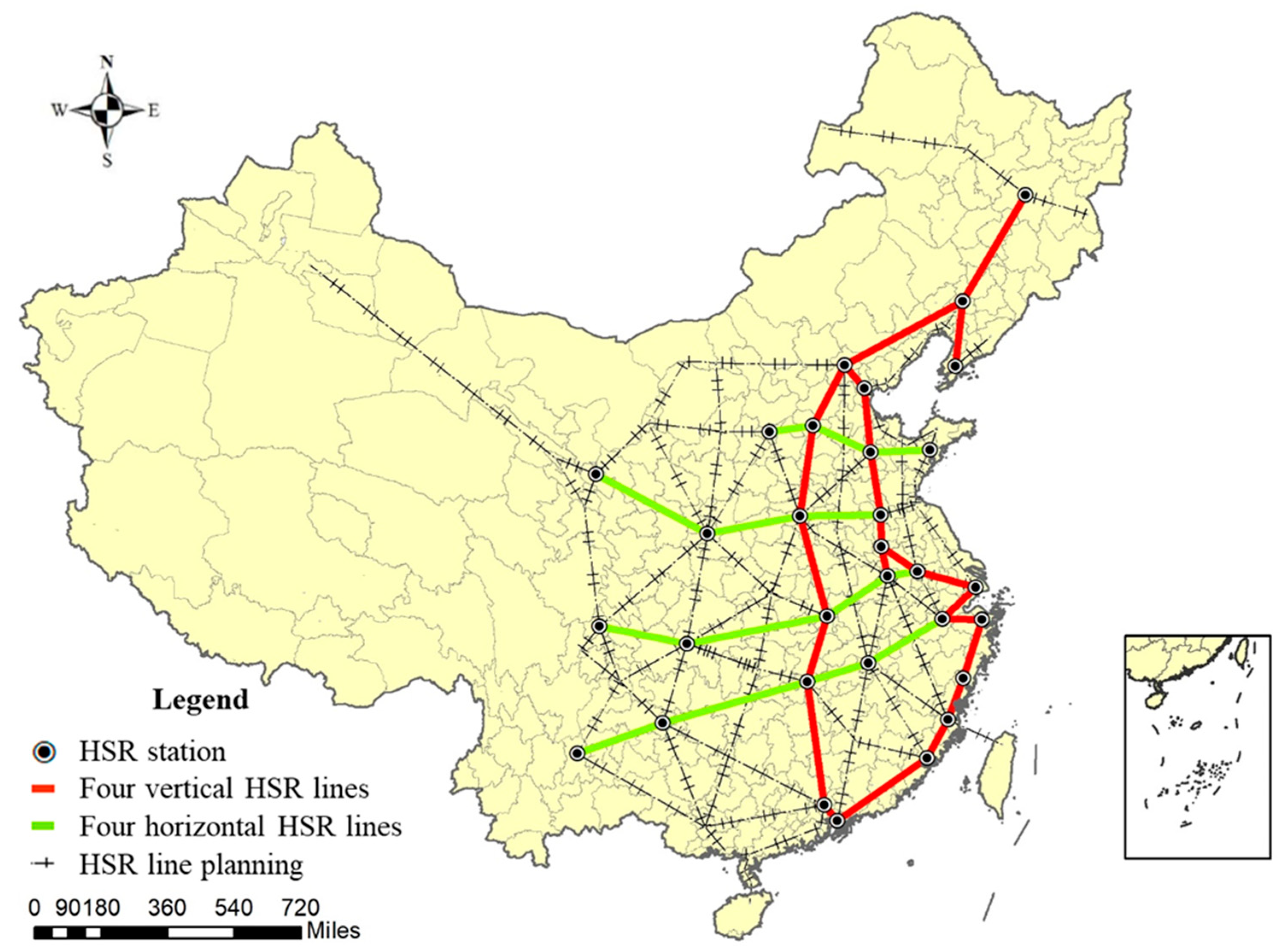
Newly lines designed for speeds above 250 km/h and upgraded existing lines for speeds of up to 200 km/h are considered as high-speed rail [1]. Although China’s HSR construction started late, its development has been fast. After about two decades of construction, China has developed the HSR with the longest operating range, largest carrying capacity and largest geographical coverage in the world. According to information from the China Railway Corporation, ever since the first HSR line started operations in 2008, China had successfully constructed 25,000 km of HSR as of 2017, thus accounting for 66.3% of the world’s total HSR length. In addition, the HSR network framework of the Four Horizontal Lines and Four Vertical Lines layout was formed (Figure 1). According to the 13th Five-Year Plan for Railway development, China’s HSR operating mileage will reach to 30,000 km, covering more than 80 percent of big cities. In addition, China will form the HSR network of Eight Horizontal Lines and Eight Vertical Lines.
Transport cost is an important factor affecting regional economic development, which can reduce trade costs and increase trade volume [2,3,4]. Among all means of transportation, HSR is particularly important and exerts a crucial impact on the economy of regions along HSR lines [5]. It is generally believed that HSR could improve accessibility, produce the time-space compression effect, facilitate the spatial (re)distribution of factor resources and exert impacts on regional economy. Accessibility refers to the convenience of using a certain transport system to reach a venue from a certain location [6]. HSR affects interactions among cities, which affect the factor agglomeration costs. Eventually, it facilitates the spatial reallocation of diverse resources, including human resources, natural resources, technology, knowledge, and information [7,8,9,10]. The reallocation effect of resources caused by HSR is known as the HSR economic distribution effect in new economic geography [11]. Such HSR economic distribution effects exist between the HSR cities and non-HSR cities, and they also exist within the cities along HSR lines. Besides that, the development of HSR also promotes the development of tourism because it is more comfortable and convenient than other modes of transportation. The research on the impact of HSR on the tourism draws much attentions and lead to fruitful achievements [12,13,14,15].
Since HSR serves primary passengers, it directly affects the service-sector the most. Differing from traditional manufacturing productions that are storable and easy for long distance transportation, the production and consumption of service products are identical in space and time [16]. The shortcoming of service sector can be alleviated by the HSR to some extent. HSR helps the cities to connect with a wider range of markets and industry chains. China has a vast territory and exhibits a marked development gradient in which there are huge differences between the economic development in East China, Central China, and West China [17,18]. Hence, balancing the development between regions is an important task [19,20]. Given China’s growing labor costs and resource environment in recent years, proactively developing the service-sector is crucial to China’s industrial transformation and upgrading [21]. On the one hand, developing the service-sector helps achieve industrial transformation. On the other hand, the service-sector agglomeration (SSA) plays three types of roles as a high-end industry: comprehensively supporting the entire industrial system, widely driving various industries, and promoting and upgrading the industrial structure [22]. In general, HSR substantially improves regional accessibility and convenience, accelerates resource flows and optimizes the spatial distribution of the service sector. Therefore, it is expected that the Chinese large-scale construction of HSR aims at: (a) balancing the differences between regional development, and (b) ensuring China’s sustained economic growth. Against the above backdrop, we attempt to tackle the following questions: How did HSR affect the SSA in cities along the HSR lines? Has the SSA been promoted or suppressed? How can one estimate such an impact reliably?
In terms of research methods, comparative method and treatment effect model are usually employed to estimate the effect of HSR. The comparative analysis method horizontally compares the economy between opened and unopened HSR cities or it longitudinally compares the economy before and after the opening of HSR, which are commonly used to estimate HSR’s impacts. A drawback of the method is that it neglects the difference between economies of cities with HSR and without HSR. It is also unable to consider the changes in the economies of non-HSR cities before and after the opening of the HSR. In recent years, scholars have used quasi-natural experiments to construct conditions that are contrary to the facts and to estimate various changes that might have occurred in economic activities without HSR. Scholars regarded the opening of the HSR as a natural experiment and set cities as experimental research subjects. The HSR cities are assigned to the treatment group, and the non-HSR cities are assigned to the control group. The difference-in-difference (DID) method is currently the most commonly used treatment effect method. Many scholars used the DID method to more accurately estimate the impacts of HSR compared to the comparative analysis method. Remarkably, the DID method requires that the treatment group and control group should experience the same impacts from common factors. In addition, the only difference between the treatment group and the control group lies in whether they are affected by HSR.
A large volume of literature focuses on whether the HSR will promote economic development and there are three views on this question. First, some studies point out that HSR can accelerates the resources flowing and promotes economic development [23,24,25,26]; Second, some studies suggest that HSR has a disadvantage on the economic development to some extent, which largely due to its high-cost of building, operating, maintaining, and so on [27,28,29,30]; Third, it is also found that HSR exerts uneven impacts across the space, which means HSR’s impacts vary across different cities or different stages of the operation of HSR. According to the New Economic Geography (NEG) theory, the improvement of transportation infrastructure will reduce transportation costs, save trading time and enhance the flow of economic activities, which facilitates the formation of the “Core-Periphery” pattern [11]. Thus, the HSR’s impact are different and multi-leveled in the various regions [31,32,33,34]. Table 1 summarized the different research findings on impacts of HSR in Asia.
In terms of the spatial structure, there may be spatial correlations between the economic indicators of different regions [35]. It is believed that the spatial spillover effect and “siphon” effect are caused by such spatial correlations. Positive spatial correlations exist if the spillover effect exceeds the “siphon” effect. Otherwise, there are negative spatial correlations. Because HSR affects the interactions among cities, it is possible that HSR can change the magnitude of such spatial correlations. One possible situation is that HSR enhances the transfer of factors from the core to the periphery in a region through the spillover effect, facilitates the development of the periphery and accelerates economic growth of the whole region. Another possible situation is that HSR accelerates the transfer of factors from the periphery to the core and that the development of the periphery is inhibited under the “siphon” effect. Whether and how much HSR influences economic development requires other supplement conditions to be met. It is difficult to evaluate the economic effect. Similarly, evaluating the impacts of HSR on the economy is not easy. It is mainly because HSR’s impacts are influenced by various factors, including the line location, construction costs, and environmental costs. In addition, it is difficult to measure the indirect effect brought by HSR effectively [36]. As a national strategic plan in China, the construction goal of HSR is to form regional fast traffic “corridors” to link the cities. Therefore, evaluating the impact of HSR is of great significance for balancing regional economy and promoting sustainable development.
In summary, although progresses have made in the research on HSR, there remain some questions to be addressed. On the one hand, little has been done regarding the spatial heterogeneity of HSR’s impacts, the transfers of regional industry and the changes in industrial spatial patterns. Because of this, existing studies rarely inspire the formulation of effective urban/regional economic policies. On the other hand, the DID method usually stacks all treatment units together. As a result, only the whole region’s effect can be estimated, and little has been done on the HSR impacts on every city. In light of the above, we employed a new counterfactual analytical method proposed by Hsiao et al. [37] (namely the HCW model) to estimate the HSR’s impact on the SSA. The characteristic of the HCW model is to assume that the objects are influenced by some common factors, but the impact of these common factors on each object is heterogeneous. Moreover, in the application of the HCW model, it does not need to measure the common factors’ impact, but to use the change of the cross-sectional correlation of the objects to evaluate the policy’s effect. This feature makes the HCW method easy to use when compared to the DID method. Therefore, this method has been widely used and achieved much in the research on the policy evaluation [38,39,40].
Based on the HCW model, we collected prefectural-level data between 1998 and 2016 to examine how the Wuhan–Guangzhou HSR (WGSHR) influences the service-sector agglomeration (SSA). To investigate the impacts of the WGSHR on SSA, we identified the control group for each city along the WGHSR. We found that the WGHSR significantly promoted the SSA along the line. However, the impacts of the WGHSR on SSA are heterogeneous. We not only enrich the quantitative research on the HSR economy but also provide extra references for planning the construction of China’s HSR and a basis for promoting the service-sector transfer and balancing regional development.
The remaining sections of this paper are arranged as follows. In Section 2, the research objects and data of the paper are described. In Section 3, we elaborate on the methodology and data. In Section 4, the results of the empirical analysis and the robustness test are reported. Section 5 consists of the conclusions and policy discussions.

2. Research Subjects and the Context

2.1. Introduction to Research Subjects

According to the information disclosed by the Ministry of Railways of China, China succeeded in operating HSR in 185 cities (referred to as prefectural-level cities, similarly hereinafter) by the end of 2016. We chose the WGHSR from numerous HSR lines to research how HSR influences the SSA. This choice has three main advantages:
(a)
The south–north WGHSR connects three provinces in Central and Southern China. As one of the longest current HSR lines in China, it passes through many cities. Compared with shorter lines, this line reveals the possible heterogeneous impacts from the HSR on the SSA.
(b)
The WGHSR has been operating for years. It takes a long time for the service-sector in a city to agglomerate. Compared with HSR lines that were constructed later, we can collect more observational data about HSR operations.
(c)
The WGHSR was opened in 26 December 2009. It is clear that 2010 will be the node from which the policy takes effect. In this way, we can avoid the problems of how to identify the effective time of the policy. The economic development level of cities along the WGHSR are shown in Table 2.
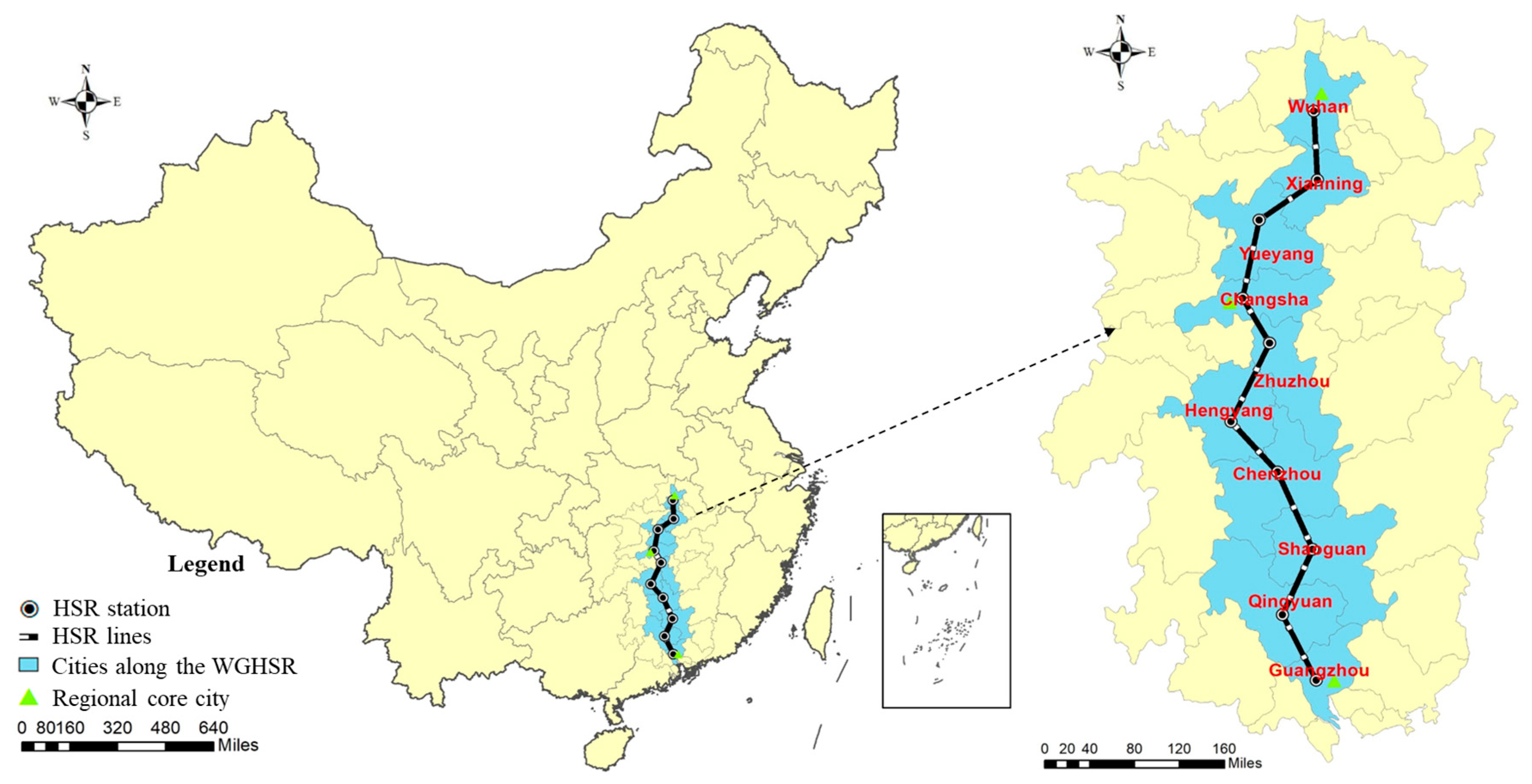
The WGHSR leaves from Wuhan and arrives in Guangzhou, running through Xianning, Yueyang, Changsha, Zhuzhou, Hengyang, Chenzhou, Shaoguan, and Qingyuan (Figure 2). This line is 1069 km long. Among all cities along the line, Wuhan, Changsha, and Guangzhou are the regional core cities. As the provincial capitals of Hubei Province, Hunan Province and Guangdong Province, respectively, the three cities have significantly higher development levels than the surrounding cities. They are economic, educational, industrial and scientific centers in their respective provinces, and exert profound impacts on surrounding cities.

2.2. Treatment Group Cities Selection

One of the challenges of using the HCW model for research lies in the endogenous problems caused by the reverse causal relationship between the HSR construction and the service-sector development. When deciding to construct an HSR line, cities with a large scale and good conditions for economic development will be given priority to construct an HSR. These cities are originally regional core cities and have a high SSA. For periphery cities, operating an HSR depends on whether the city is located on the path between the regional core cities. In other words, the development of a periphery city is not a direct cause of deciding whether the HSR passes through that city. It is thus reasonable to regard the opening of the WGHSR as a quasi-natural experiment and eliminate the regional core cities along the line. The result of the treatment group cities’ selection is shown in Table 3.

2.3. Candidate Control Group Cities Selection

The candidate control group cities selection is another crucial problem of using the HCW model. The employment of the HCW model lies in two conditions. First, the cities in the candidate control group should be relevant to the treatment group cities in the development of the service-sector. Second, the service-sector development in the candidate control group cities should be kept independent from the opening of the HSR. For this reason, we selected the candidate control group cities from 294 cities nationwide based on the following conditions and three reasons. (a) We eliminated 185 cities that have opened an HSR by the end of 2016. If the candidate control group contains cities with HSR, it will fail to achieve the counterfactual analysis, which apparently does not meet the requirements for analysis. (b) We eliminated cities that have undergone huge adjustments in administrative areas. To avoid the shock of urban area changes on SSA, we did not include another 36 cities where the administrative area changed by over 500 km2 during the study period in account. (c) We eliminated another 36 cities within 100 km from the HSR city. The existence of the HSR spatial spillover effect [41,42,43,44] makes it impossible to choose the cities that have not opened an HSR but are close to HSR cities into a candidate control group. Based on the above operations, we limited the external shocks as much as possible and eventually chose the remaining 37 cities as the candidate control group cities.

3. Methodology and Data Description

3.1. A Brief Introduction of the HCW Model

In this section, we briefly summarize the panel data evaluation method of HCW. As is known, it is impossible to observe the results where an individual is both affected and not affected by an incident at the same time. For example, it is reasonable to observe the development of the HSR city and the non-HSR city by some means. On the contrary, it is impossible to observe the non-HSR city’s development under the assumption that the non-HSR city with HSR service. Neither does it observe the HSR city’s development under the assumption that the HSR city without HSR service. Without the loss of generality, we hypothesized that other individuals except Individual 1 are all not affected by the incident. y i t is the dependent variable, i denotes the observed individual, t denotes the observation time, y ˜ t = ( y 2 t , · · · , y N t ) , t ranges from 1 to T, T 1 is the time when the incident occurs, and the results where the individual is not affected are recorded as y i t 0 . Correspondingly, the affected result is recorded as y i t 1 as follows:
y i t = y i t 0 i = 1 , 2 , · · · , N ,   t = 1 , 2 , · · · , T 1
y i t = { y i t 1     i = 1 y i t 0     i = 2 , · · · , N   ,   t = T 1 + 1 , · · · , T
The HCW model hypothesizes that the relevance between individuals is driven by certain common factors. When they are not affected by the above incident, all individuals including individual 1 should obey the following model:
y i t 0 = α i + λ i f t + ε i t   i = 1 , 2 , · · · , N ,   t = 1 , 2 , · · · , T 1
where α i is the individual effect, f t is the unknown common factor which is a k-dimensional column vector, λ i is the load parameter, ε i t is the error item, and E ( ε i t ) = 0 . After the incident takes effect, it is it is necessary to estimate the difference between y 1 t 1 and y 1 t 0 when t = T 1 + 1 , · · · , T , namely, the treatment effect Δ ^ 1 t = y 1 t 1 y 1 t 0 , in order to estimate the impact of the incident on individual 1. Because y 1 t 1 is observable and y 1 t 0 is unobservable, it is thus necessary to obtain the estimated value of y 1 t 0 , namely, y 1 t 0 ^ . As usual, the common factor is unknown. Although it is difficult to find f t , laws can be determined based on observing the relevant individuals who are not affected by the incident. As long as these relevant individuals are driven by a common factor and have a stable structure, f t may be replaced by a synthesis of the relevant individuals to evaluate the counterfactual paths of individual 1. It is the core idea of the HCW model and the foundation of evaluating the impacts of HSR on SSA. It has proved that Equation (3) can be rewritten as follows in the given conditions:
y 1 t 0 = α 1 + θ ˜ y ˜ t t = 1 , 2 , · · · , T
where α 1 is the individual effect of Individual 1, y ˜ t is the relevant individuals who are relevant to the Individual 1 and not affected by the incident. θ ˜ is the estimation value of the load parameter.
Because the location entropy (LE) describes the professionalism of the service-sector in a city, we take LE as a research variable to access the impacts of HSR on SSA. The calculation formula of LE is as follows:
L E i t = ( e i t s / e i t ) / ( e t s / e t )
where L E i t is the service-sector LE of city i in year t. e i t s is the value added of the service-sector of city i in year t. e i t is the added value of all industries of city i in year t. e t s is the added value of the national service-sector in year t. e t is the added value of all industries of the country in year t. In this article, Equation (3) can be rewritten as follows:
L E 1 t 0 = α + θ L E ˜ t t = 1 , 2 , · · · , T
Based on such settings, it is possible to estimate the counterfactual paths for SSA in each treatment group city when t = T 1 + 1 , · · · , T , even if common factors are unknown. First, we estimate α ^ and θ ˜ ^ when t = 1 , 2 , · · · , T 1 . Second, we calculate L E ˜ t when t = T 1 + 1 , · · · , T and then obtain the L E ^ 1 t 0 of the potential paths. Lastly, we assess the net effect of how HSR affects the SSA as Δ ^ 1 t = L E 1 t 1 L E 1 t 0 ^ and its confidence interval Δ ^ 1 t ± c σ L E 1 t 0 . The average treatment effect (ATE) of HSR can be calculated by the following formula:
ATE 1 = 1 ( T T 1 ) t = T 1 + 1 T Δ 1 t ^ t = T 1 + 1 , T 1 + 2 , · · · , T
The conditions of using the HCW model is that a certain synthesis of the candidate control group (optimal synthetic control group) cities can be fit well into the treatment group cities. There are many methods and criterion for fitting. Following the research of Hsiao et al. [38], we use the ordinary least square (OLS) method to fit the optimal synthetic control group of every treatment group city. The estimation procedures are as follows.
(a)
Fit the LE’s trend of every WGHSR city before the opening of HSR, which provides the basis for predicting the LE’s trend after the opening of the HSR. Select j ( j = 1 , , N ) cities randomly from the candidate control group cities (Section 2.3) and take the LE before the WGHSR opened as the independent variables. Take the LE of a city belonging to a control-group as the dependent variable (suppose City A) during the same period for OLS regression. In this way, we can get N city groups, which contain j cities of each group.
(b)
Apply the Akaike information criterion (AIC) [45] to select the certain city group with the smallest value as the optimal synthetic control group corresponding to City A. The AIC is an estimator of the relative quality of statistical models for a given set of data. Given a collection of models for the data, AIC estimates the quality of each model, relative to each of the other models. Thus, AIC provides a means for model selection. Specifically, compare the AIC of every model and select the smallest as the optimal synthetic control group corresponding to City A.
(c)
Repeat from Procedure (a) to Procedure (b) for each city in the treatment group and compare the predicted LE and the actual LE to estimate the HSR’s impact on the SSA along the WGHSR.
Compared to the comparative analysis method and the DID method, the HCW method is easy to use which dues to its efficient on constructing the optimal synthetic control group. As a coin has two sides, it should be noted that the prediction process of the SSA index is based on just one single variable which may not be effective to reflect the complex relationship between different cities. Therefore, the results of this research need robustness test which will be introduced later.

3.2. Descriptive Statistical Analysis

The annual average LE of the service-sector in cities along the WGHSR line from 1998–2016 is listed in Table 4. There are two research findings. (1) The LE of the five cities among the treatment group cities decreased and the other two cities increased. Chenzhou enjoyed the largest decrease of 21.88% and Qingyuan enjoyed the largest increase of 26.39%. (2) The treatment group cities generally enjoyed a decrease of 4.54%, while the control group cities enjoyed a decrease of 8.49%. The former was approximately 4% lower than the latter. Based on the rough judgment of the abovementioned data, the SSA of cities along the WGHSR experienced different changes. According to the analysis of Section 1, HSR can accelerate the distribution speed and widen the range of the factor resource distribution, which significantly affected the spatial distribution of the service-sector. Affected by spatial correlations, HSR plays two roles. One the one hand, it enhances the transfer of factor resources from regional core cities to regional periphery cities and facilitates the development and agglomeration of service industries in some cities under the spillover effect. On the other hand, HSR accelerates the transfer of factor resources from regional periphery cities to regional core cities and restricts the development and agglomeration of the service-sector in some cities under the “siphon” effect. How HSR affects the agglomeration of the service-sector depends on the tendency of regional development. In the next section, we employed the method introduced in Section 3 and evaluated the net impact of HSR on the SSA.

4. Results of Empirical Analysis

4.1. HCW Model Results and Analysis

Instead of adopting the past method of mixing research on all control group cities, we researched cities one by one. Based on establishing the optimal control-group cities synthesis for each control group city, we evaluated how the WGHSR affects the SSA along the line. The impact is measured by the differences between the actual LE value and synthetic value.
Taking Xianning as an example, we first choose the city one by one from the 37 candidate control group cities and took the LEs from 1998–2009 as the independent variables. Then, we took the LE of Xianning during the same time as the dependent variable for the OLS regression. Depending on the AIC, we found the city synthesis with the smallest AIC and used it as the optimal synthetic control group. Then, we observed the fitting effect of the optimal synthetic control group on Xianning. Similarly, we used the same analysis step to get the fitting effect of the other six control group cities (Table 5).
Table 5 shows the performance of the fitting with the HCW model. In general, adj. R 2 and the F statistics are the most common index to reflect the fitting effect of the OLS model. The adj. R 2 of the 7 treatment group cities are all similar to 0.999 which reflects that obtained good fitting effects and the differences between the actual value and the synthetic one are all within 1‰. The F statistics are big and significant at the level of 1% which can draw the same conclusion. These provide the conditions to simulate the counterfactual when an HSR is not constructed.
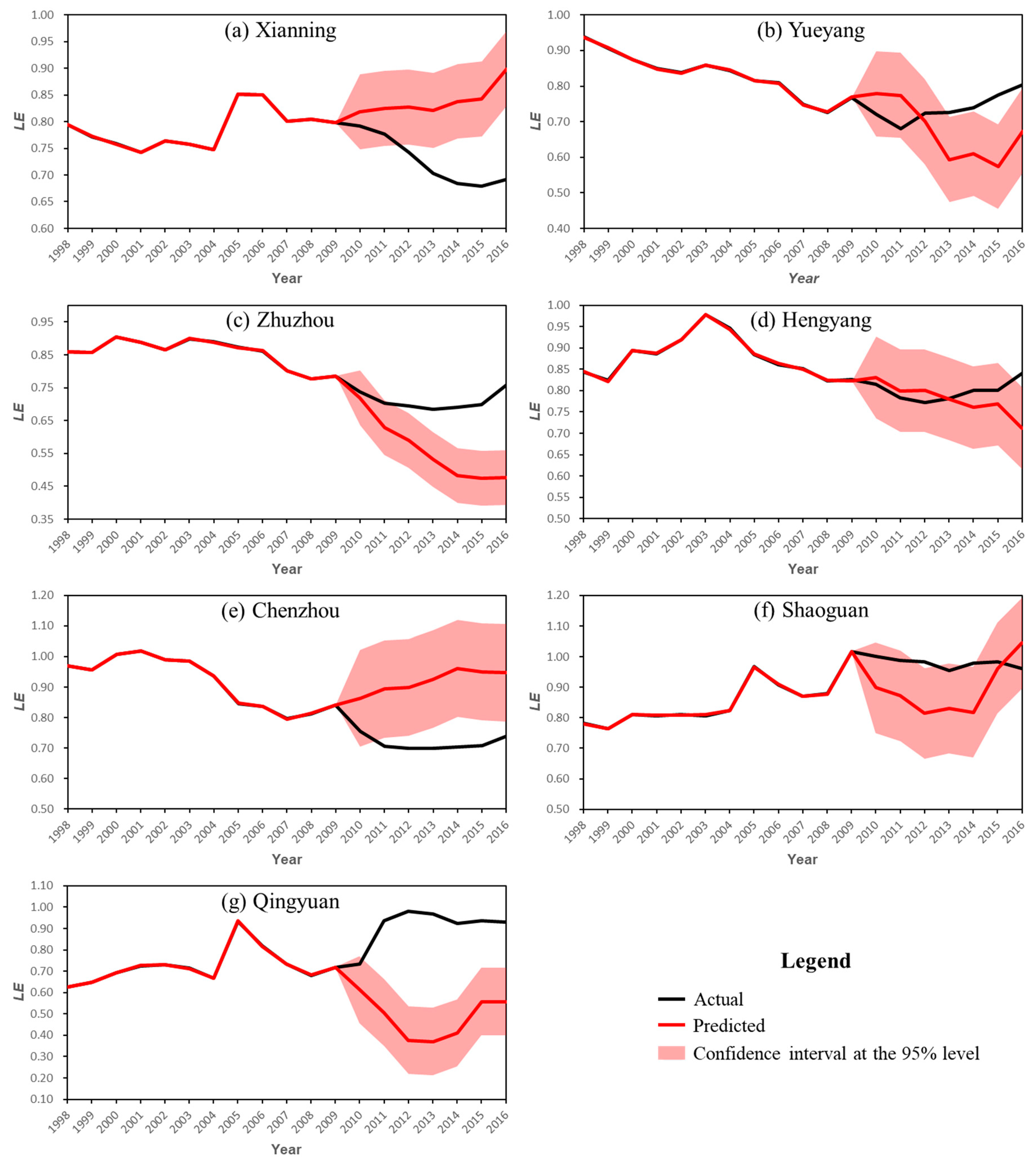
Furthermore, Figure 3 shows the trend of the actual value and synthetic value of the LE of each treatment group city from 1998–2016. The black line reflects the actual trend of the LE, the red line reflects the synthetic trend accordingly, and the red shadow is the confidence interval at the 95% level. We can find that the actual trend and synthetic trend of the seven treatment group cities between 1998 and 2009 are highly anastomosis. After the WGHSR was opened in 2010, there were different deviations between the actual values and synthetic values. In addition, taking Xianning as an example, the actual value and synthetic value were close before the HSR was opened. After the HSR opened, the actual value was significantly lower than the synthetic value and even below the lower limit of the 95% level. Based on observing and summarizing the information in Figure 3, we divided the seven cities into three groups. The first group includes Xianning and Chenzhou. The actual value of this group is significantly lower than the synthetic value. The second group includes Zhuzhou and Qingyuan. The actual value of this group is significantly higher than the synthetic value. The third group includes Yueyang, Hengyang and Shaoguan. The actual value and synthetic value of this group are not significantly different.
Then, we calculate the ATE of the seven cities based on Equation (7) (Table 6). According to the table mentioned above, the operation of the WGHSR improves the LE of Qingyuan and Zhuzhou by 88.96% and 27.18%, respectively. On the other hand, it restricted the LE of Chenzhou and Xianning by 22.18% and 13.63%, respectively. The impacts on Yueyang, Hengyang, and Shaoguan were insignificant. Overall, the WGHSR increased the LE along the HSR by 9.44%. Thus, it is thought that the impact of the HSR on the SSA in HSR cities is spatially heterogeneous. This conclusion is consistent with the theoretical analysis mentioned above. However, the conclusion is slightly inconsistent with the research results of [25,46]. They studied the China Yangtze River Delta in China using the DID method and thought that the HSR did not inhibit the SSA. We conducted a detailed and careful analysis of this and found the reason for the result as follows. According to Jean Gottmann’s opinion, the China Yangtze River Delta is one of the world’s six largest city agglomerations. All cities in these regions have a huge impetus for development under the radiance of the regional core city [47,48]. In addition, this region is also one of the regions with the highest HSR density in the world. Given that regional economic activities are so close, the spatial spillover effect and economic externality of HSR exert a profound impact on the cities along the HSR line. In other words, partial cities in the region without HSR are still substantially affected by the operations of the HSR. If these cities are taken as samples of the control group, it negatively affects the requirements of the DID method, which requires that the control group is not affected by policy. As a result, it may result in low estimation of the HSR effect. We try to avoid this problem to make the estimation more persuasive.

4.2. Robustness Check

According to the above research findings, the impacts of the WGHSR on the SSA in cities along the line are spatially heterogeneous. However, is this characteristic caused by the opening of the HSR? Is it accidental? Is this phenomenon caused by some unobserved external factors, such as the investment scale of local governments and the adjustment of industrial policies? To eliminate interferences and contingency from other factors, we adopted the following robustness tests.
Robustness test 1: Placebo Test
To verify that the policy effect is indeed due to the impact of the policy itself rather than other factors, we adopted the placebo test proposed by Abadie et al. [49] to verify the results. The basic idea of the placebo test is as follows. First, select a non-HSR city and suppose the city opened an HSR in 2010. Second, fit this city’s potential path of LE with the HCW model. If the WGHSR does affect the SSA along the HSR, such differences should be small under the above operations. We conducted the placebo test in all cities of the optimal synthetic control group. One of the reasons is that there are strong correlations between the treatment group cities and the optimal synthetic control group cities. Another reason is that each treatment group city corresponds to five to seven optimal synthetic control group cities. Multiple tests ensure the persuasiveness of the placebo test. According to this idea, the placebo test was performed one by one for the seven treatment group cities.
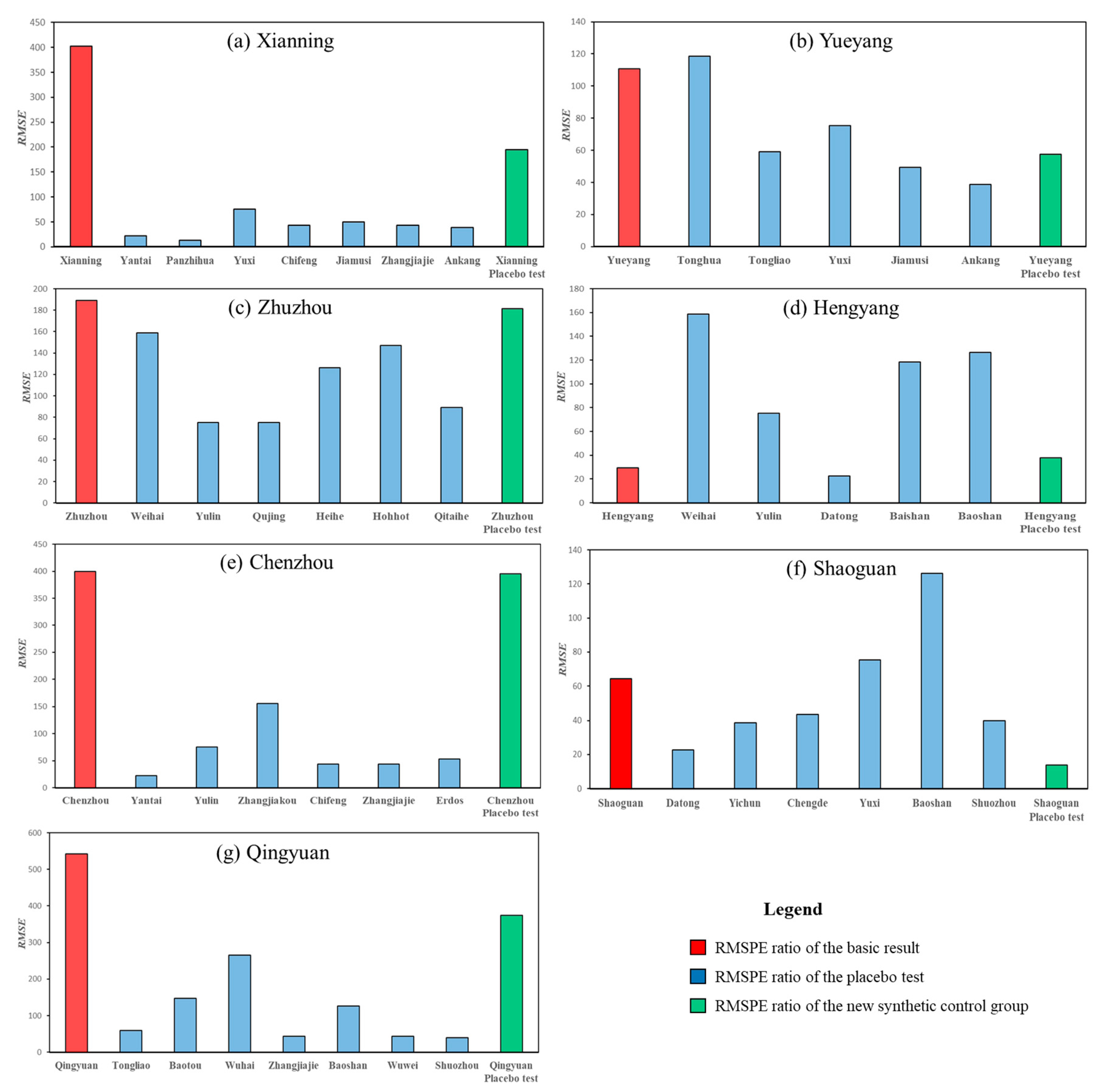
Moreover, to measure the differences between the actual value and synthetic value, we calculate the root mean square prediction error (RMSPE) value. The calculation formula of the RMSPE is ( 1 T 0 t = 1 T 0 ( L E 1 t α θ L E ˜ t ) 2 ) 1 2 . The post-period RMSPE represents the fitted degree after the HSR opened. Pre-period RMSPE refers to the fitted degree before the HSR opened. In consideration of the fact that a high pre-period RMSPE value is unable to reflect the effect of the HSR, we choose to represent the differences through a ratio. The RMSPE ratio is equal to (post-period RMSPE/pre-period RMSPE). As mentioned above, we should pay attention to the RMSPE ratio index which because a high pre-period RMSPE value is unable to reflect the effect of the HSR. Figure 4 shows the RMSPE ratio of the benchmark result and the robustness test. The red histogram is the RMSPE ratio that corresponds to the benchmark conclusion. The blue histogram refers to the RMSPE ratio based on the placebo test of the benchmark conclusion. The green histogram is the RMSPE ratio that corresponds to another robustness test that will be illustrated later.
We also take Xianning as example to describe the placebo test result. It can be found from Figure 4a that the red histogram is higher than all the 7 blues ones. Specifically, the HSR’s impact on SSA for Xianning is significantly higher than the 7 non-HSR cities in the assumption of opened HSR. In this way, we can find that the WGHSR has the significant impact on SSA for Xianning, Zhuzhou, Chenzhou, Qingyuan (Figure 4a,c,e,g), respectively). This result is basically consistent with that in Table 6 verifying the robustness of the benchmark results.
Robustness test 2: replace the synthetic control group
According to the requirements of the HCW model, there is no strict constraint on the fitting degree. Therefore, we re-fitted the counterfactual paths by changing the optimal synthetic control group cities. If the counterfactual path severely deviates from results in Section 4.1, after changing the optimal synthetic control group, it means that the benchmark conclusion is not robust. Otherwise, it cannot reject the robustness of the benchmark conclusion.
Based on the above analysis, Table 7 is produced which shows the new optimal synthetic control group of every treatment group city as well as the fitted effect. We also take Xianning as example to clearly describe the robustness test. The adj. R 2 is 0.9988 when Tongliao, Yulin, Hegang, Baishan, Hohhot, Liupanshui, and Baoshan formed the new optimal synthetic control group. The difference between the actual value and the new synthetic value is at the level of 1%. The F statistic is 1332 and significant as the level of 1%. The two indexes show that a good fitting is also achieved.
Moreover, according to the results of Table 8, the new ATE of Xianning from 2010 to 2016 was −0.1074 and the HSR restricted the SSA by 12.91%. After conducting the same analysis of the remaining treatment group cities, we find that the results in Table 7 and Table 8 are basically consistent with those in the benchmark one.
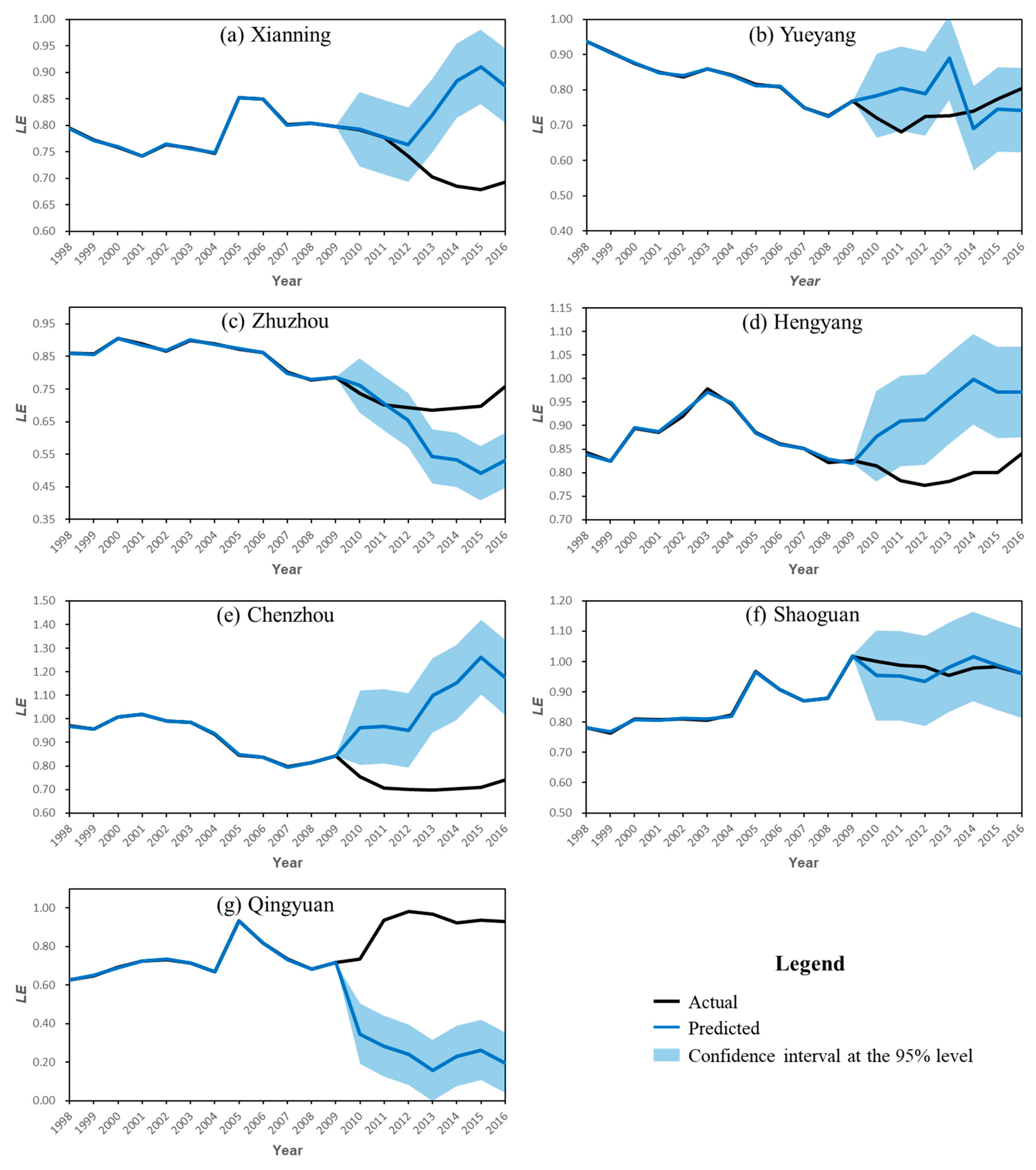
Figure 5 is the graph of using the new optimal synthetic control group to fit the treatment group cities. After comparing to the Figure 3, two conclusions can be drawn: (1) The synthetic LE of all the 7 cities are very similar to the actual one before 2009, which means every treatment group city is fitted well after replace the optimal synthetic control group cities; (2) There is basically no difference about the results between the benchmark analysis and the robustness analysis. Considering all these results, the WGHSR has a significant impact on SSA for Xianning.
The same as Yueyang, we adopted the HCW model to analyze Yueyang through the above analysis step. A good fitting was achieved when Weihai, Hegang, Heihai, Wuhai, Liupanshui, and Zhangjiajie formed the new optimal synthetic control group. We determined that there were no significant differences between the actual LE and synthetic LE after the HSR opened. The result is consistent with the benchmark result. Judging from the robustness test, the HSR did not exert any significant impact on the SSA in Yueyang.
It is necessary to illustrate that according to the information in Figure 5, we determined that the actual LE of Hengyang is significantly lower than the synthetic LE after replacing the optimal synthetic control group, which is inconsistent with the benchmark result. We think that for Hengyang itself, the impact of the HSR on its SSA is not significant for Hengyang itself. Therefore, the replacement of the optimal synthetic control group cannot fit counterfactual paths well. This is represented in the fact that the RMSPE ratio of the benchmark result and of the new synthetic control group are both smaller than those of the placebo test shown in Figure 4. Overall, there are basically no differences between the benchmark result and robustness test. Based on the abovementioned analysis, it is thought that evaluating how the WGHSR affects the SSA is robust and effective.
Robustness test 3: replace the SSA index
In this paper, the estimation of the common factor relationship that is then used to determine the counterfactual is probable insufficiently robust based on just one single variable. To ensure the reliability of the result, we employ other SSA indexes, i.e., employment density (ED) in service sector and service sector product per capita (SSPPA), to study the WGHSR’s impact by using the HCW method. If there is little difference between the results, then we can ensure that the above results are reliable.
Table 9 represents the ATE of every city along the route and the whole line. As compared to the Table 6 and Table 8, it is found that there is little difference between them except Yueyang. The ATE of Yueyang about ED index is 0.0591, and about SSPPA index is −0.0467. Even so, both changes are not significant for Yueyang. Thus, it also shows that the result is reliable.

5. Conclusions and Policy Implications

As HSR significantly reduces the restrictions of spatial distance on the flows of factor resources, it exerts a profound impact on the service-sector with fast flows of factor resources. Although scholars have been concerned that HSR can significantly affect the distribution of the service-sector, there are still some deficiencies in the existing studies. Because it is difficult to assess the impacts of HSR, there is no accurate conclusion at present. In this paper, prefectural-level data from 1998 to 2016 and a panel data program evaluation method are employed to evaluate the effect of the Wuhan–Guangzhou HSR (WGHSR) on the SSA along the route. Specifically, we predict the SSA index of the HSR cities along the route in the absence of the HSR using the SSA index in selected non-HSR cities. In order to achieve this, we identify the optimal control group for each city along the WGHSR and calculate the potential SSA index. By comparing the predicted index and the actual index, the evaluation of the WGHSR’s impact on the SSA can be obtained. Two robustness tests show that out conclusions are robust.
According to the research findings, the WGHSR has increased SSA significantly. However, we also find that the impacts of the WGHSR on SSA are heterogeneous. We believe that WGHSR has brought about both the spillover effect and the “siphon” effect. On the one hand, HSR increases the flow of factor resources from regional core cities to regional periphery cities and facilitates the development and agglomeration of service industries in some cities under the spillover effect. On the other hand, HSR accelerates the transfer of factor resources from marginal regions to core cities and facilitates the development and SSA under the “siphon” effect. It should be noted that every econometric method has its limitations. The HCW method is easy to use which dues to it is efficient on constructing the optimal synthetic control group of every HSR city along the WGHSR. The prediction process of the SSA index is based on just one single variable which may not be effective to reflect the complex relationship between different cities. Therefore, the conclusions of this research still need follow-up study and further confirmation by relevant studies.
In the context of energetic efforts of HSR construction, whether a city gives play to its advantages is the key to ensuring its development. Based on our findings, we propose the following policy advice.
First, enhance the planning of constructing HSR networks and further perfect current HSR networks. As an important means of transportation between cities, HSR is characterized by fast speed and convenience, which brings huge revolutions to urban development. In addition, HSR has typical network economic effects and the impact of one HSR line in a region on the industrial layout is limited. Only when forming an HSR network will the effects on regional economic development be more significant. To achieve this objective, the HSR network should be planned scientifically. It is thus necessary to enhance the planning of constructing HSR networks from the perspective of enhancing inter-city economic connections and accelerating regional economic integration. It is the precondition of achieving a reasonable layout and facilitating economic development in all cities.
Second, relying on HSR implements differentiated regional development strategies. The impact of HSR on the regional economy is spatially heterogeneous. It is necessary for all regions to enhance their connections with other regions, give full play to advantageous industries and facilitate development based on HSR. In addition, small cities should be good at seizing opportunities and accurately positioning and developing their advantageous characteristic industries to achieve differentiated competition. Moreover, big cities should enhance the efforts of undertaking international high-end industries and actively transfer out low-end industries to make room for industry upgrades. Furthermore, big cities should vigorously support the development of the service-sector and form complementary advantages between regions.
Third, the government should oversee possible market failures in HSR development and facilitate regional economic development on the principle of ensuring both efficiency and fairness.
Author Contributions

T.L. conceived and designed the study; M.T. collected and analyzed the data; M.T. and Y.W. wrote the manuscript; S.Y. and S.F. reviewed and edited the manuscript.

Funding

This research is supported by the MOE (Ministry of Education in China) Project of Humanities and Sciences (Project No. 18YJCZH029).

Acknowledgments

The authors are grateful to the editors and the anonymous reviewers for their insightful comments and suggestions.

Conflicts of Interest

The authors declare no conflict of interest. The founding sponsors had no role in the design of the study; in the collection, analyses, or interpretation of data; in the writing of the manuscript, and in the decision to publish the results.

References

  1. UIC. General Definitions of High Speed; International Union of Railways: Paris, France, 2008; Available online: https://uic.org/highspeed#What-is-High-speed-rail (accessed on 9 April 2019).
  2. Atack, J.; Bateman, F.; Haines, M.; Margo, R.A. Did railroads induce or follow economic growth? Urbanization and population growth in the American Midwest, 1850–1860. Soc. Sci. Hist. 2010, 34, 171–197. [Google Scholar] [CrossRef]
  3. Donaldson, D. Railroads of the Raj: Estimating the impact of transportation infrastructure. Am. Econ. Rev. 2018, 108, 899–934. [Google Scholar]
  4. Donaldson, D.; Hornbeck, R. Railroads and American economic growth: A “market access” approach. Q. J. Econ. 2016, 131, 799–858. [Google Scholar] [CrossRef]
  5. Givoni, M. Development and impact of the modern high-speed train: A review. Transp. Rev. 2006, 26, 593–611. [Google Scholar] [CrossRef]
  6. Morris, J.M.; Dumble, P.L.; Wigan, M.R. Accessibility indicators for transport planning. Transp. Res. Part A Gen. 1979, 13, 91–109. [Google Scholar] [CrossRef]
  7. Ureña, J.M.; Menerault, P.; Garmendia, M. The high-speed rail challenge for big intermediate cities: A national, regional and local perspective. Urban Plan. Int. 2009, 26, 266–279. [Google Scholar]
  8. Blanquart, C.; Koning, M. The local economic impacts of high-speed railways: Theories and facts. Eur. Transp. Res. Rev. 2017, 9, 12. [Google Scholar] [CrossRef]
  9. Guirao, B.; Campa, J.L.; Casado-Sanz, N. Labour mobility between cities and metropolitan integration: The role of high speed rail commuting in Spain. Cities 2018, S0264275117312520. [Google Scholar] [CrossRef]
  10. Li, H.; Tjia, L.; Hu, S. Agglomeration and Equalization Effect of High Speed Railway on Cities in China. J. Quant. Tech. Econ. 2016. [Google Scholar] [CrossRef]
  11. Krugman, P. Geography and Trade; The MIT Press: Cambridge, UK, 1991. [Google Scholar]
  12. Pagliara, F.; Mauriello, F.; Garofalo, A. Exploring the interdependences between High Speed Rail systems and tourism: Some evidence from Italy. Transp. Res. Part A Policy Pract. 2017, 106, 300–308. [Google Scholar] [CrossRef]
  13. Guirao, B.; Campa, J.L. The effects of tourism on HSR: Spanish empirical evidence derived from a multi-criteria corridor selection methodology. J. Transp. Geogr. 2015, 47, 37–46. [Google Scholar]
  14. Chen, Z.; Haynes, K.E. Tourism Industry and High Speed Rail—Is There a Linkage: Evidence from China’s High Speed Rail Development; Social Science Electronic Publishing: Rochester, NY, USA, 2012. [Google Scholar]
  15. Chen, Z.; Haynes, K.E. Impact of high-speed rail on international tourism demand in China. Appl. Econ. Lett. 2015, 22, 57–60. [Google Scholar]
  16. LI, W.-X.; Li-Wen, T. Two Dimension Evaluation Model of Services Agglomeration and Its Experience Study—The Case of American Service. China Ind. Econ. 2008. [Google Scholar] [CrossRef]
  17. Ye, X.; Xie, Y. Re-examination of Zipf’s law and urban dynamic in China: A regional approach. Ann. Reg. Sci. 2012, 49, 135–156. [Google Scholar]
  18. Dai, Q.; Ye, X.; Wei, Y.D.; Ning, Y.; Dai, S. Geography, ethnicity and regional inequality in Guangxi Zhuang autonomous region, China. Appl. Spat. Anal. Policy 2018, 11, 557–580. [Google Scholar] [CrossRef]
  19. Wei, Y.D.; Ye, X. Beyond convergence: Space, scale, and regional inequality in China. Tijdschr. Econ. Soc. Geogr. 2009, 100, 59–80. [Google Scholar]
  20. Xu, X.; Wang, Y.; Tao, L. Comprehensive evaluation of sustainable development of regional construction industry in China. J. Clearn Pord. 2019, 211, 1078–1087. [Google Scholar] [CrossRef]
  21. Zhao, M.; Liu, X.; Derudder, B.; Zhong, Y.; Shen, W. Mapping producer services networks in mainland Chinese cities. Urban Stud. 2015, 52, 3018–3034. [Google Scholar]
  22. Knox-Hayes, J. The developing carbon financial service industry: Expertise, adaptation and complementarity in London and New York. J. Econ. Geogr. 2009, 9, 749–777. [Google Scholar] [CrossRef]
  23. Jun, L.; Jitao, S.; Yusheng, L.; Jie, X. The simulation of spatial distribution patterns of China’s HSR-economic zones based on the 2D time-space map. Acta Geogr. Sin. 2013, 68, 147–158. [Google Scholar]
  24. Chen, Z.; Haynes, K.E. Impact of high-speed rail on regional economic disparity in China. J. Transp. Geogr. 2017, 65, 80–91. [Google Scholar] [CrossRef]
  25. Shao, S.; Tian, Z.; Yang, L. High speed rail and urban service industry agglomeration: Evidence from China’s Yangtze River Delta region. J. Transp. Geogr. 2017, 64, 174–183. [Google Scholar]
  26. Wetwitoo, J.; Kato, H. Inter-regional transportation and economic productivity: A case study of regional agglomeration economies in Japan. Ann. Reg. Sci. 2017, 59, 321–344. [Google Scholar]
  27. De Rus, G.; Nombela, G. “Is Investment in High Speed Rail Socially Profitable?”. J. Transp. Econ. Policy 2007, 41, 3–23. [Google Scholar]
  28. Zhao, J.; Zhao, Y.; Li, Y. The variation in the value of travel-time savings and the dilemma of high-speed rail in China Transp. Res. Part A Policy Pract. 2015, 82, 130–140. [Google Scholar]
  29. Wu, J.; Nash, C.; Wang, D. Is high speed rail an appropriate solution to China’s rail capacity problems? J. Transp. Geogr. 2014, 40, 100–111. [Google Scholar] [CrossRef]
  30. Wang, K.; Xia, W.; Zhang, A. Should China further expand its high-speed rail network? Consider the low-cost carrier factor Transp. Res. Part A Policy Pract. 2017, 100, 105–120. [Google Scholar]
  31. Kim, H.; Sultana, S. The impacts of high-speed rail extensions on accessibility and spatial equity changes in South Korea from 2004 to 2018. J. Transp. Geogr. 2015, 45, 48–61. [Google Scholar] [CrossRef]
  32. Diao, M. Does growth follow the rail? The potential impact of high-speed rail on the economic geography of China. Transp. Res. Part A Policy Pract. 2018, 113, 279–290. [Google Scholar] [CrossRef]
  33. Jia, S.; Zhou, C.; Qin, C. No difference in effect of high-speed rail on regional economic growth based on match effect perspective? Transp. Res. Part A Policy Pract. 2017, 106, 144–157. [Google Scholar] [CrossRef]
  34. Qin, Y. ‘No county left behind?’ The distributional impact of high-speed rail upgrades in China. J Econ. Geogr. 2017, 17, w13. [Google Scholar] [CrossRef]
  35. Anselin, L. Spatial econometrics: Methods and models. Studies in Operational Regional Science; Springer: Dordrecht, The Netherlands, 1998. [Google Scholar]
  36. Elhorst, J.P.; Oosterhaven, J. Integral cost-benefit analysis of Maglev projects under market imperfections. J. Transp. Land Use 2008, 1, 65–87. [Google Scholar] [CrossRef]
  37. Hsiao, C.; Steve Ching, H.; Ki Wan, S. A panel data approach for program evaluation: Measuring the benefits of political and economic integration of Hong Kong with mainland China. J. Appl. Econom. 2012, 27, 705–740. [Google Scholar] [CrossRef]
  38. Gobillon, L.; Magnac, T. Regional Policy Evaluation: Interactive Fixed Effects and Synthetic Controls. Rev. Econ. Stat. 2013, 98, 535–551. [Google Scholar]
  39. Bai, C.E.; Qi, L.; Min, O. Property taxes and home prices: A tale of two cities. J. Econ. 2014, 180, 1–15. [Google Scholar]
  40. Li, H.; Qi, L.; Shi, Y. Determining the number of factors when the number of factors can increase with sample size. J. Econ. 2017, 197, 76–86. [Google Scholar]
  41. Easterly, W.; Rebelo, S. Fiscal policy and economic growth. J. Monet. Econ. 1993, 32, 417–458. [Google Scholar] [CrossRef] [Green Version]
  42. Krugman, P.; Elizondo, R.L. Trade policy and the third world metropolis. J. Dev. Econ. 1996, 49, 137–150. [Google Scholar]
  43. Yu, H.; Hong-Chang, L. The Estimate of Transport Hub Level and Its Spatial Spillover Effects—A Spatial Panel Data Study on China’s Prefecture-level City. China Ind. Econ. 2015. [Google Scholar] [CrossRef]
  44. Zhang, X. Has transport infrastructure promoted regional economic growth?—with an analysis of the spatial spillover effects of transport infrastructure. Soc. Sci. China 2013, 34, 24–47. [Google Scholar]
  45. Akaike, H. Information Theory and an Extension of the Maximum Likelihood Principle. In Selected Papers of Hirotugu Akaike; Springer: New York, NY, USA, 1998; pp. 199–213. [Google Scholar]
  46. Deng, T.; Wang, D.; Cheng, S. The Impact of High Speed Railway on Urban Service Industry Agglomeration. J. Financ. Econ. 2017, 43, 119–132. [Google Scholar]
  47. Li, W.; Wang, W.; Wang, Y.; Ali, M. Historical growth in total factor carbon productivity of the Chinese industry–a comprehensive analysis. J. Clean. Prod. 2018, 170, 471–485. [Google Scholar] [CrossRef]
  48. Wu, C.; Wei, Y.D.; Huang, X.; Chen, B. Economic transition, spatial development and urban land use efficiency in the Yangtze River Delta, China. Habitat Int. 2017, 63, 67–78. [Google Scholar]
  49. Abadie, A.; Diamond, A.; Hainmueller, J. Synthetic control methods for comparative case studies: Estimating the effect of California’s tobacco control program. J. Am. Stat. Assoc. 2010, 105, 493–505. [Google Scholar]
Figure 1. China high-speed rail (HSR) network framework.
Sustainability 11 02128 g001
Figure 2. Station locations of the Wuhan–Guangzhou HSR (WGHSR).
Sustainability 11 02128 g002
Figure 3. Trend of the LE of the treatment group cities.
Sustainability 11 02128 g003
Figure 4. Root mean square prediction error (RMSPE) ratio of the benchmark result and robustness test.
Sustainability 11 02128 g004
Figure 5. Trend of LE in the treatment group cities after replacing the optimal synthetic control group.
Sustainability 11 02128 g005
Table 1. Different research findings on impacts of HSR in Asia.
StudyRegionMethodsConclusionExplanation
Lu et al. (2013) [23]ChinaComparative analysisPromotive effectHSR has helped to save 34% of the transportation time for five economic regions in China and 50% of the time for inter-city traffic in the 2-h economic circle.
Chen and Haynes (2017) [24]ChinaComparative analysisPromotive effectThe regional economic disparity has decreased since the development of HSR. HSR has promoted regional economic convergence in China.
Shao et al. (2017) [25]ChinaDIDPromotive effectHSR has a positive effect on the urban service industry agglomeration of the cities located along the rail lines. Higher levels of HSR service intensity have a greater effect on urban service industry agglomeration.
Wetwitoo and Kato (2017) [26]JapanComparative and regression analysisPromotive effectThe influence of HSR on economic productivity is higher in regions with HSR stations, particularly those located within a 150–200 km radius from the largest cities
Zhao et al. (2015) [28]ChinaComparative analysisNegative effectThe HSRs in China have no comparative advantage over sleeper trains in long distance travel. Large scale HSR construction faces great market risk and economic loss.
Wu et al. (2014) [29]ChinaComparative analysisNegative effectAt existing Chinese values of time, new conventional lines are generally a better solution to Chinese railway capacity problems than high speed rail.
Wang et al. (2017) [30]ChinaComparative analysis and DIDNegative effectIn the low-density corridors especially in the central and western China, low-cost carriers (LCCs) might leave HSR with little survival room in the long run
Kim and Sultana (2015) [31]KoreaComparative analysisUnbalanced effectThe advantages of expanding the HSR network are limited to the initial HSR corridors, which deepened the inequalities in accessibility between regions.
Diao (2018) [32]ChinaComparative analysis and DIDUnbalanced effectCities in the wealthy eastern region and with HSR access enjoy higher accessibility benefits compared with cities in the hinterland and without direct HSR access.
Jia et al. (2017) [33]ChinaDIDUnbalanced effectChina’s HSR construction has a positive effect on economic growth and will become an important force in reshaping the organization of China’s spatial economy. However, the effect is different for different high-speed rail lines.
Qin (2017) [34]ChinaDIDUnbalanced effectComparing GDP and GDP per capita of counties located on the affected railway lines to counties located on other railway lines, there is a 3–5% significant reduction in GDP and GDP per capita after the HSR operation.
Table 2. GDP per capita of cities along the Wuhan–Guangzhou line (2016).
No.Prefectural-Level CityProvinceGDPPC of 2016 (USD)
1WuhanHubei16,782
2XianningHubei6628
3YueyangHubei8255
4ChangshaHunan18,687
5ZhuzhouHunan9346
6HengyangHunan5874
7ChenzhouHunan7029
8ShaoguanGuangdong6231
9QingyuanGuangdong5440
10GuangzhouGuangdong21,368
Note: (1) The data are collected from the China City Statistical Yearbook (2017). (2) The GDPPC are converted by the annual average exchange rate of 6.6423 RMB/USD.
Table 3. Results of the treatment group cities selection.
No.Prefectural-Level CityIncluded (Yes/No)
1WuhanNo
2XianningYes
3YueyangYes
4ChangshaNo
5ZhuzhouYes
6HengyangYes
7ChenzhouYes
8ShaoguanYes
9QingyuanYes
10GuangzhouNo
Table 4. Changes in location entropy (LE) of service sector before and after the Wuhan–Guangzhou line was opened.
GroupCityBefore Opening (1998–2009)After Opening (2010–2016)Changes (%)
Treatment GroupXianning0.78670.7242−7.9453
Yueyang0.83130.7384−11.1766
Zhuzhou0.85530.7093−17.0737
Hengyang0.87800.7991−8.9843
Chenzhou0.91650.7160−21.8751
Shaoguan0.85410.978714.5834
Qingyuan0.72450.915726.3915
Group average0.83520.7973−4.5378
Control GroupGroup average0.87320.7991−8.4860
Table 5. Summary of fitting performance.
No.CityOptimal Synthetic Control GroupFitting Effect
Adj. R 2 F Statistics
1XianningYantai, Panzhihua, Yuxi, Chifeng, Jiamusi, Zhangjiajie, Ankang0.99986827 ***
2YueyangTonghua, Tongliao, Yuxi, Jiamusi, and Ankang0.99943529 ***
3ZhuzhouWeihai, Yulin, Qujing, Heihe, Hohhot, Qitaihe0.99891708 ***
4HengyangWeihai, Yulin, Datong, Baishan, Baoshan0.9973828.8 ***
5ChenzhouYantai, Yulin, Zhangjiakou, Chifeng, Zhangjiajie, Ordos0.999919,200 ***
6ShaoguanDatong, Yichun, Chengde, Yuxi, Baoshan, Shuozhou0.99861306 ***
7QingyuanTongliao, Baotou, Wuhai, Zhangjiajie, Baoshan, Wuwei, Shuozhou0.99974987 ***
Note: *** represents the significance at 1% level.
Table 6. Summary of the average treatment effect.
No.CityATEChanges (%)Significant (Yes/No)
1Xianning−0.1143−13.6275Yes
2Yueyang0.06649.8789No
3Zhuzhou0.151627.1787Yes
4Hengyang0.02022.5931No
5Chenzhou−0.2040−22.1765Yes
6Shaoguan0.08719.7655No
7Qingyuan0.431188.9633Yes
8Group average0.06619.4402-
Table 7. Summary of the fitting effect after replacing the optimal synthetic control group.
No.CityOptimal Synthetic Control GroupFitting Effect
Adj. R 2 F Statistics
1XianningTongliao, Yulin, Hegang, Baishan, Hohhot, Liupanshui, Baoshan0.99881332 ***
2YueyangWeihai, Hegang, Heihe, Wuhai, Liupanshui, Zhangjiajie0.99851192 ***
3ZhuzhouBaotou, Yichun, Baishan, Jiamusi, Zhangjiajie, Ankang0.9952384.5 ***
4HengyangYantai, Baotou, Yichun, Heihe, Zhangjiakou0.9877177.1 ***
5ChenzhouBaicheng, Yulin, Baishan, Zhangjiakou, Wuhai, Liupanshui, Shiyan0.99963807 ***
6ShaoguanBaotou, Hohhot, Panzhihua, Wuhai, Jiamusi, Ankang0.9976771.3 ***
7QingyuanDatong, Hohhot, Panzhihua, Yuxi, Liupanshui, Chifeng, Shiyan0.99851070 ***
Note: *** represents the significance at 1% level.
Table 8. Summary of the average treatment effect in the robustness test.
No.CityATEChanges (%)Significant (Yes/No)
1Xianning−0.1074−12.9148Yes
2Yueyang−0.0396−5.0901No
3Zhuzhou0.106117.5906Yes
4Hengyang−0.1434−15.2153No
5Chenzhou−0.3660−33.8249Yes
6Shaoguan0.00890.9178No
7Qingyuan0.6708273.8480Yes
8Group average0.075910.9936-
Table 9. Summary of the average treatment effect of the employment density (ED) and service sector product per capita (SSPPA) indexes. ATE: average treatment effect.
No.CityEDSSPPA
ATESignificant (Yes/No)ATESignificant (Yes/No)
1Xianning−0.1378Yes−0.1549Yes
2Yueyang0.0591No−0.0467No
3Zhuzhou0.1853Yes0.1449Yes
4Hengyang0.0492No−0.0184No
5Chenzhou−0.2896Yes−0.4109Yes
6Shaoguan0.0476No0.0118No
7Qingyuan0.7763Yes0.7639Yes
8Group average0.0614-0.0863-