Article

Application of Nonnegative Tensor Factorization for Intercity Rail–Air Transport Supply Configuration Pattern Recognition

1
MOT Key Laboratory of Transport Industry of Big Data Application Technologies for Comprehensive Transport, Beijing Jiaotong University, Beijing 100044, China
2
College of Air Traffic Management, Civil Aviation University of China, Tianjin 300300, China
3
Tianjin Sub-bureau of Air Traffic Management, Tianjin 300300, China
*
Author to whom correspondence should be addressed.
Sustainability 2019, 11(6), 1803; https://doi.org/10.3390/su11061803
Submission received: 5 January 2019 / Revised: 27 February 2019 / Accepted: 20 March 2019 / Published: 25 March 2019

Abstract

:
With the rapid expansion of the railway represented by high-speed rail (HSR) in China, competition between railway and aviation will become increasingly common on a large scale. Beijing, Shanghai, and Guangzhou are the busiest cities and the hubs of railway and aviation transportation in China. Obtaining their supply configuration patterns can help identify defects in planning. To achieve that, supply level is proposed, which is a weighted supply traffic volume that takes population and distance factors into account. Then supply configuration can be expressed as the distribution of supply level over time periods with different railway stations, airports, and city categories. Furthermore, nonnegative tensor factorization (NTF) is applied to pattern recognition by introducing CP (CANDECOMP/PARAFAC) decomposition and the block coordinate descent (BCD) algorithm for the selected data set. Numerical experiments show that the designed method has good performance in terms of computation speed and solution quality. Recognition results indicate the significant pattern characteristics of rail–air transport for Beijing, Shanghai, and Guangzhou are extracted, which can provide some theoretical references for practical policymakers.

1. Introduction

As a scheduled service, railway and aviation play a major role in intercity transportation. In the emerging market of China, both the railway and aviation industry have grown rapidly in the last 30 years. Since 2005, China has become the second largest air travel market in the world. By the end of 2013, the total operation mileage of China’s high-speed railways (HSR) has become the longest in the world. Furthermore, the HSR network is still developing rapidly. According to the long-term railway network plan, the Chinese HSR network will have 38,000 km of passenger dedicated lines in operation and about 80% of China’s domestic aviation market will be overlapped by HSR lines by 2025 [1].
Air transport has the advantage in long-distance intercity travel due to its shorter travel time. However, with continuous expansion of the HSR network, many studies found that the entry of HSR puts competition pressure on airlines in terms of passenger demand and airfares [2]. Competition and cooperation are the two main perspectives when comparing these two modes of transportation. Studies regarding these two perspectives are fruitful. Jiang and Zhang [3] analyzed the effects of cooperation between a hub airline and an HSR operator when the hub airport may be capacity-constrained. Results show hub capacity plays an important role in assessing the welfare impact of airline–HSR cooperation. Roman and Martin [4] conducted a discrete choice experiment to better understand passenger preferences. They found that reducing connecting time by schedule coordination is crucial. Takebayashi [5] explored the possibility of collaboration between airport and HSR to improve the airport’s gateway function. Their results showed that congestion at the bigger demand airports can be reduced through collaboration between HSR and the smaller demand airports. Jiang and Zhang [6] investigated the long-term impacts of HSR competition on airlines and pointed out that HSR competition can induce the airline to adopt a network structure closer to the social optimum. Chen [7] discovered that the deployed HSR services have a significant substitutional effect on domestic air transport in China, but the effect varies across different HSR routes, travel distances, and city types. Yang et al. [8] adopted the origin-destination (OD) passenger flow data to compare the spatial configurations of the Chinese urban system, and results showed they differ greatly in HSR networks and in air networks. Marti-Henneberg. [9] proposed a method to calculate the capacity to attract users to HSR stations by comparing potential demand between them. This helped to establish a reasonable way of allocating financial resources for public investment. The results also emphasized the need to encourage improved intermodality around railway stations. Escobari. [10] employed the random-coefficients logit methodology to allow a general alternative model to estimate the various demand systems for airport, airline, and departure time choice. The results showed that passengers are more inclined to choose different airlines than changing airports and departure times.
Built on the existing studies, this paper will apply the nonnegative tensor factorization (NTF) to extract supply configuration patterns of intercity rail–air transport from different city classifications for departure and arrival, respectively. The supply configuration in this paper is expressed by the distribution of a weighted supply traffic volume for different railway stations, airports, and city categories that takes OD population and distance factors into account over a designated period. For better interpretability and computational efficiency, the CANDECOMP/PARAFAC (CP) decomposition and block coordinate descent (BCD) algorithm are adopted, respectively. It is demonstrated in the numerical experiments that the designed method can extract the required patterns with concise form while realizing good performance in computation speed and solution quality.
The remainder of this paper is organized as follows. Section 2 Study Area, Data and Methodology outlines the data and research methods. Section 3 Patterns Recognition Results presents the extracted supply configuration patterns. In Section 4 Result Analysis, the different patterns are discussed by comparison between them. Section 5 Conclusion concludes the study and suggests some future works.

2. Study Area, Data, and Methodology

2.1. Study Area and Data Sources

Our study focuses on the intercity rail–air transport supply configuration pattern of three megacities (Beijing, Shanghai, and Guangzhou with urban populations of over 15 million). All their rail–air departure and arrival traffic schedules are required.
The cities studied are cities with flights and trains to Beijing, Shanghai, and Guangzhou. The classification of cities is mainly based on the annual passenger enplanements of their airports. The first category is the hub airports of Beijing, Shanghai, and Guangzhou. According to the statistical standards of Civil Aviation Administration of China, the second and third categories are airports where passenger enplanements are more than 1% and 0.2% to 1% of the total volume of passenger enplanements in the country, respectively. The remaining airports in cities is the fourth category.
In addition, an HSR coverage ratio is introduced to illustrate the proportion of HSR connections in the corresponding categories as not all the cities studied are connected to the HSR network. The details of cities’ (airports) categories are shown in Table 1.
The study area comprises 4 airports and 150 flight connected cities, 11 railway stations, and 348 railway connected cities in mainland China. Data on each city’s urban population are extracted from the National Urban Population and Construction Land by City on the website of the Ministry of Housing and Urban-Rural development of the People’s Republic of China (MOHURD) [11]. The flight schedule data of CAT1′s airports were collected on 21 January 2018. A total of 5046 flight plans were captured. To compare the railway supply, international flights are not included. Therefore, the total number of flights captured is 3649.
Moreover, flight number, aircraft type, departure airport, destination airport, estimated departure time, estimated arrival time in flight schedule were available, and information, such as flight traffic volume, estimated departure and arrival time, OD airports, is used for data mining. Correspondingly, the data on OD city pairs, rail travel time (in minutes), travel distance (in kilometers), and daily frequency of Beijing, Shanghai, and Guangzhou trains for the same day were obtained from two official websites: www.12306.cn [12] (the official online booking site for all trains in China) and www.gaotie.cn [13] (the website dedicated to HSR travel in China). Train numbers for Beijing, Shanghai, and Guangzhou were 909, 879, and 1204, respectively.

2.2. Nonnegative Tensor Factorization

Tensors are generalizations of matrices, and a tensor can be seen as a multi-dimensional array. For instance, a 1st-order tensor is a vector, and a 2nd-order tensor is a matrix. To effectively extract the supply configuration pattern from the constructed tensors, nonnegative tensor factorization (NTF) is utilized, which is a generalization of nonnegative matrix factorization (NMF) [8]. NTF has many advantages, such as strong interpretability (due to nonnegative factors) and small storage space, and is widely used in the field of data mining [14].
In our study, three dimensions representing different factors including the studied airports and railway stations, the connected city’s classification, and time periods, construct the tensors for departure and arrival, respectively. The entries of the tensors which denote the supply level of the trips are calculated according to Equation (1). The population of the connected city and the straight-line distance to the connected city are taken into account for describing the supply level. By connecting more people in a larger distance, the supply level is assumed to be enhanced. In other words, the supply level of different trips is treated differently: with the same distance, a larger connected population indicates higher supply level; with the same population, a longer connected distance means a higher supply level.
d 1 , d 2 , d 3 = P b max ( P ) D a , b max ( D a , : ) S d 1 , d 2 , d 3
d 1 , d 2 , d 3 is the entry of the constructed tensor in which d 1 is determined by the studied airport and railway stations of city a ; d 2 is determined by the classification of the connected city b , and d 3 is determined by the time period departing from/arriving at the studied city a . Specifically, each time period is 30 min, and there are a total of 48 time periods in this paper. S d 1 , d 2 , d 3 is the transportation supply (i.e., number of flights and trains included in the specified time period) between the studied city a and the connected city b . P b represents the population of the connected city b and max ( P ) returns the maximum population of the connected cities; D a , b is the distance between the studied city a and the connected city b , and max ( D a , : ) returns the longest distance between the studied city a and all connected cities.
According to different research needs, NTF is divided into different decomposition methods, such as CP decomposition [15,16] and Tucker decomposition [17]. In this study, we apply CP decomposition because of its better interpretability. It decomposes the original tensor into several factor matrices which can imply the features of each factor on different patterns [18]. The optimization problem is proposed as Equation (2).
min f ( F 1 , , F N ) = 1 2 | | F 1 F 2 F N | | 2 subject   to   + d 1 × d 2 × × d N , F i + d i × R , i = 1 , , N
in which is the original tensor; d i ( i = 1 , 2 , , N ) represents the dimensions of the original tensors; F i is the factorized matrix which describes the relationship between factor i and potential patterns, and we call them “pattern scores” in this paper, i.e., different columns of F i give the pattern scores corresponding to factor i for different patterns; R is a specified order which is the number of the potential patterns; represents outer product operation.
To compute the CP decomposition effectively, many algorithms have been proposed by researchers. In this paper, a block coordinate descent (BCD) method proposed by Xu and Yin [18] was adopted due to its outstanding performance in both speed and solution quality. See researches [18,19,20] for further details on matrix calculation. Through iterative computation, several potential patterns with more concise form can be extracted.

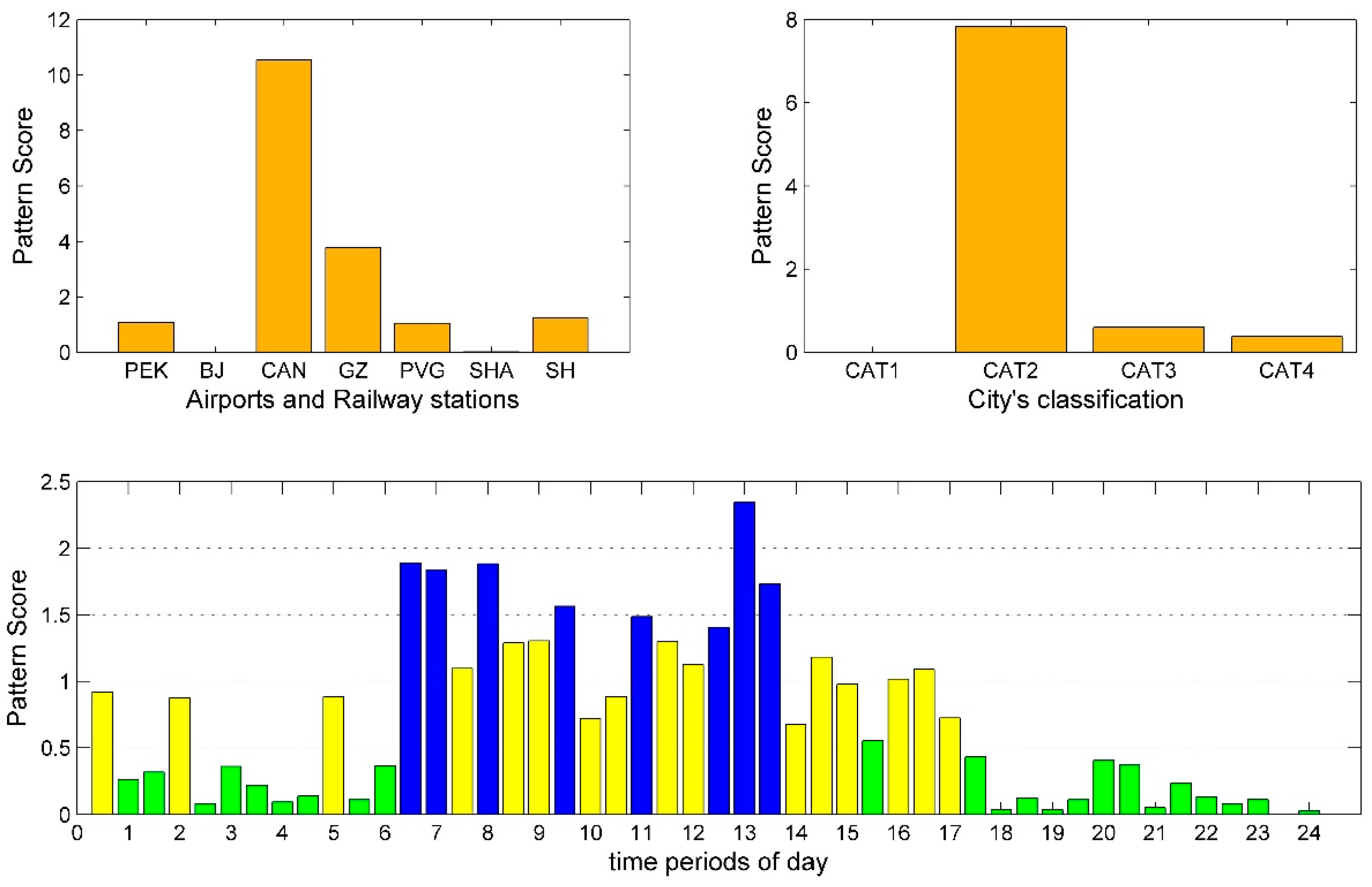
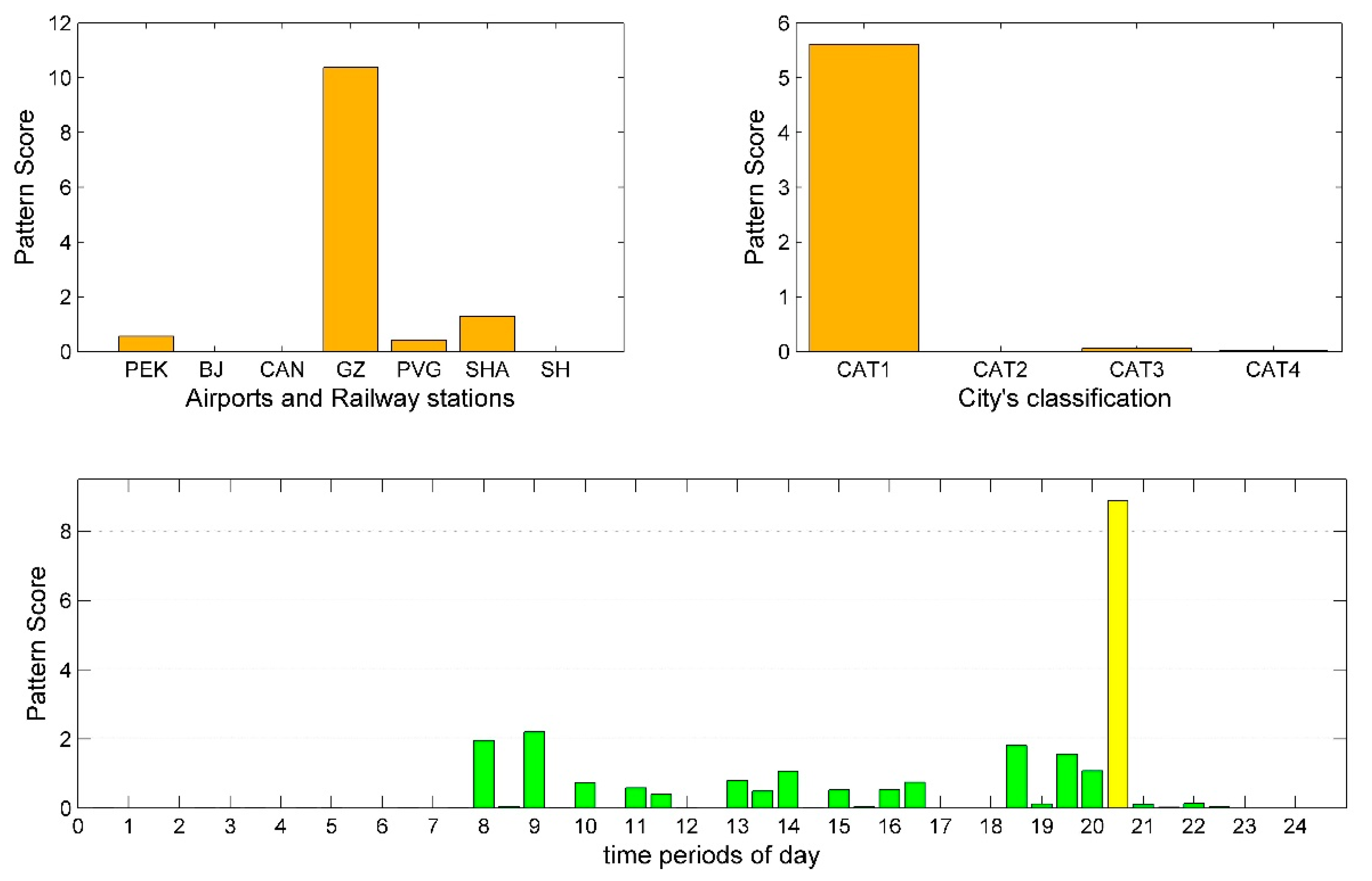
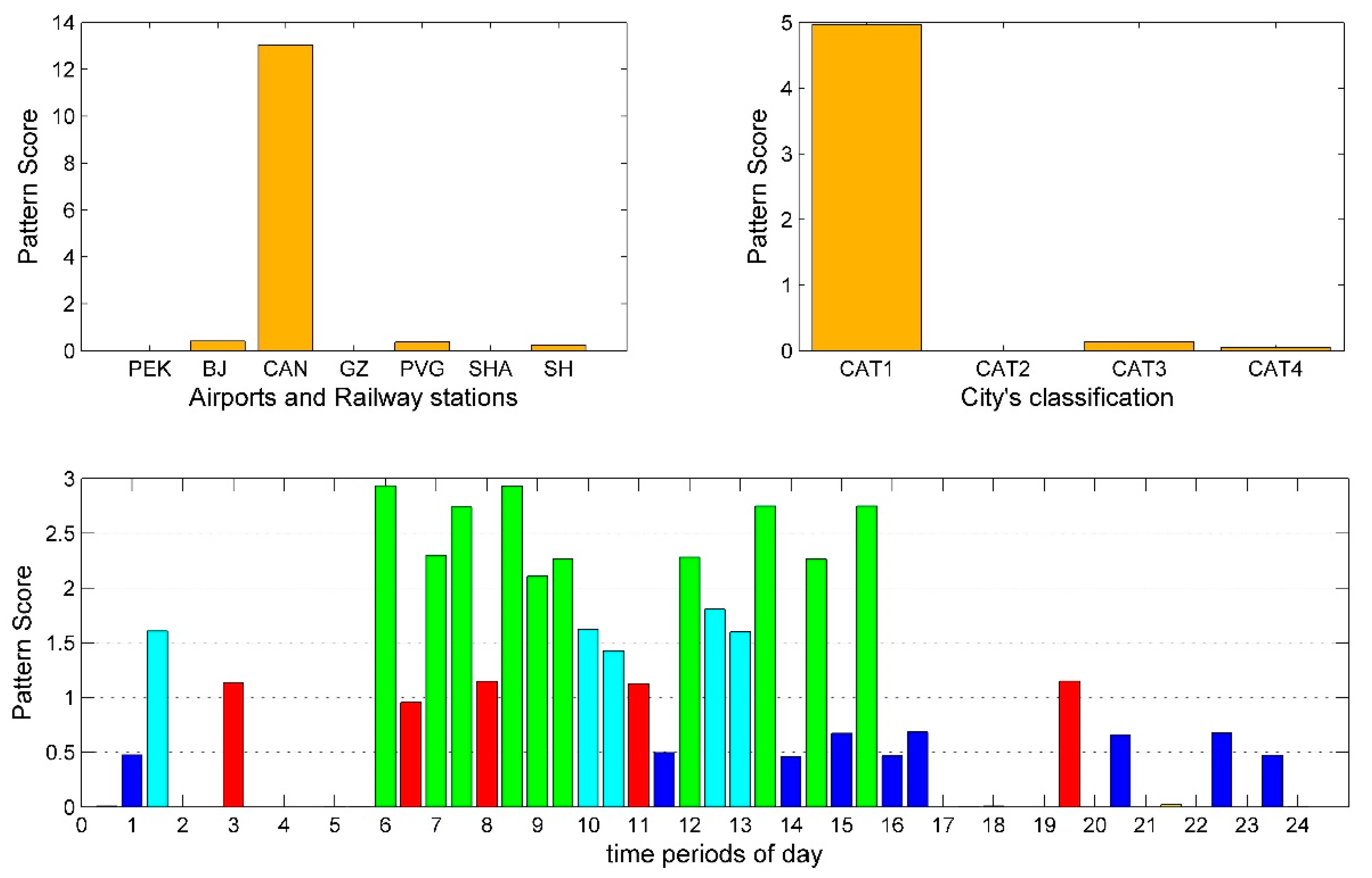
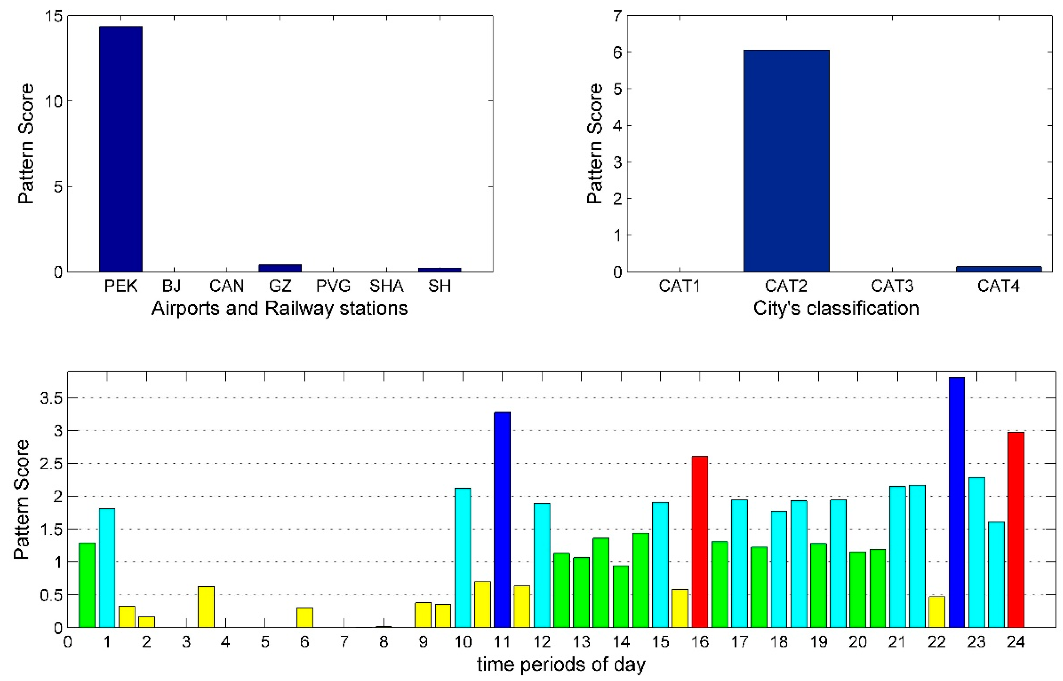
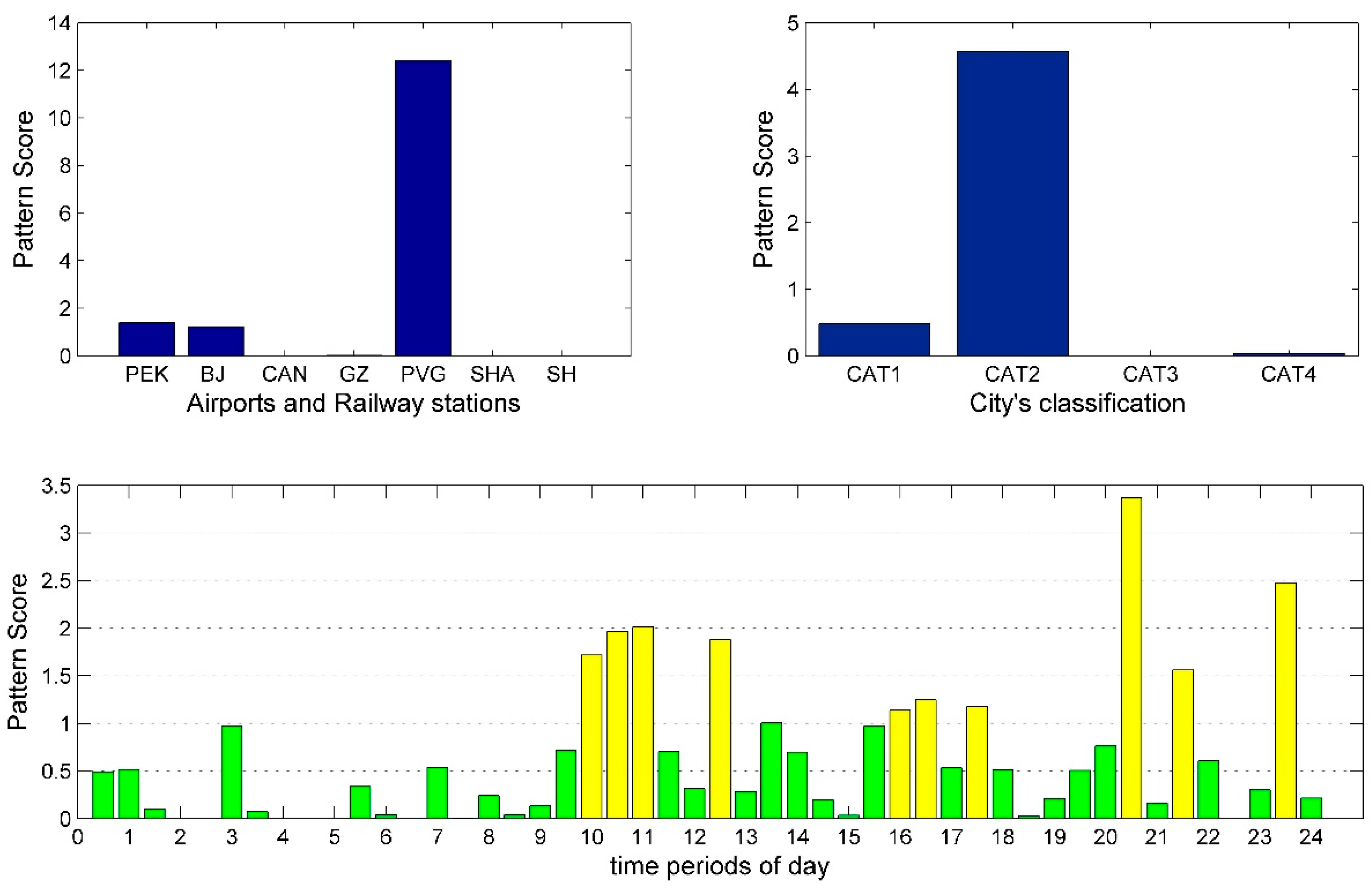
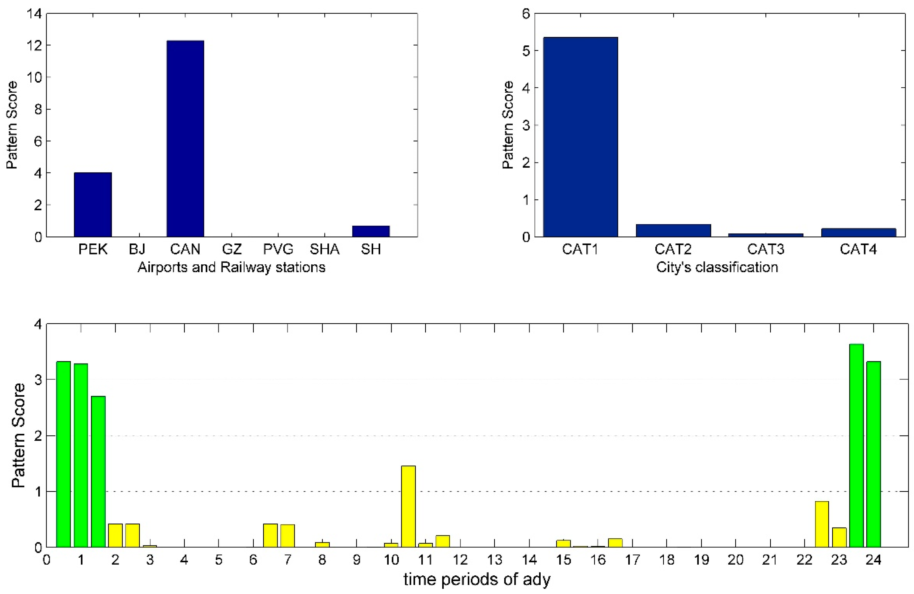
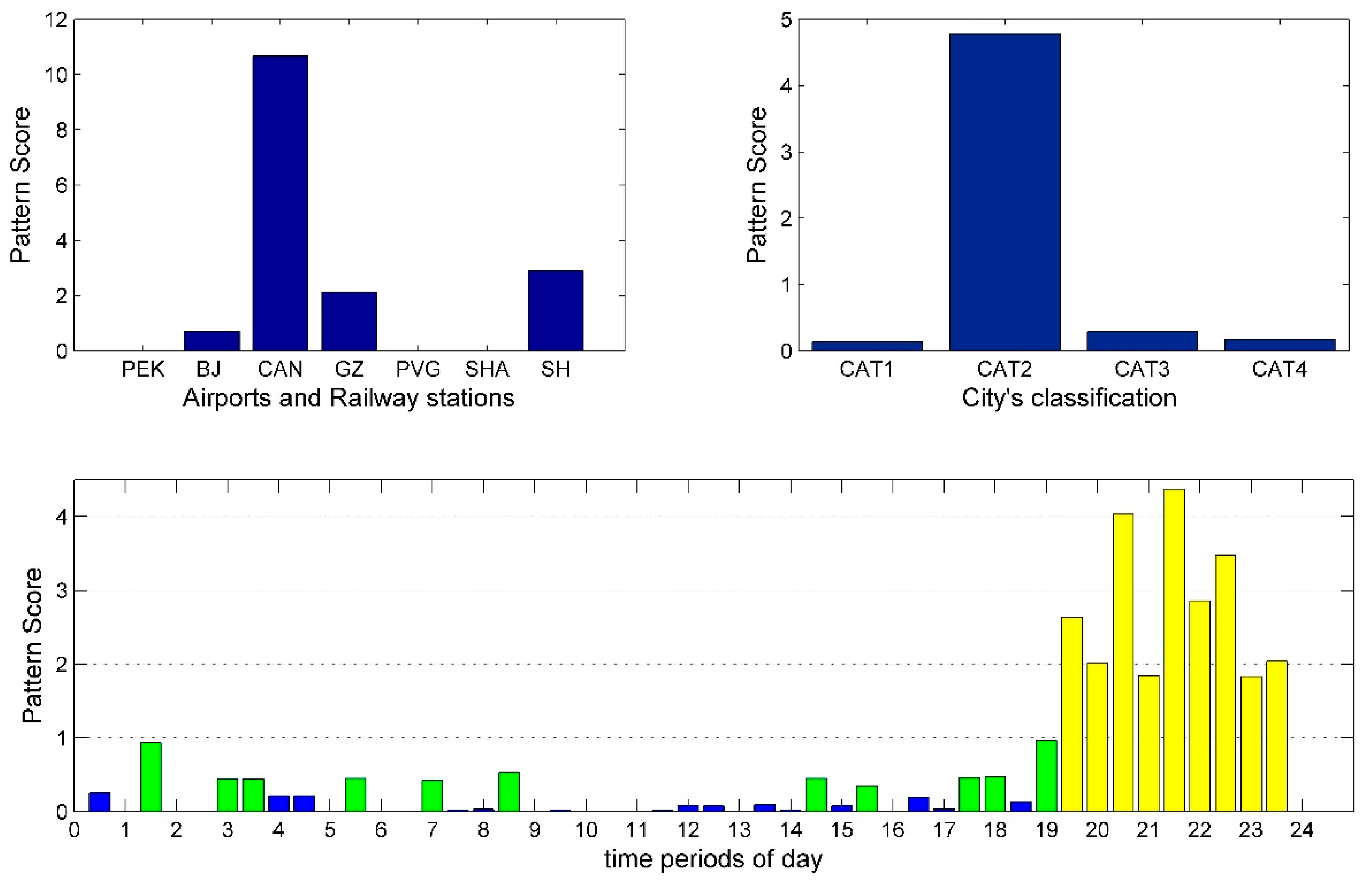
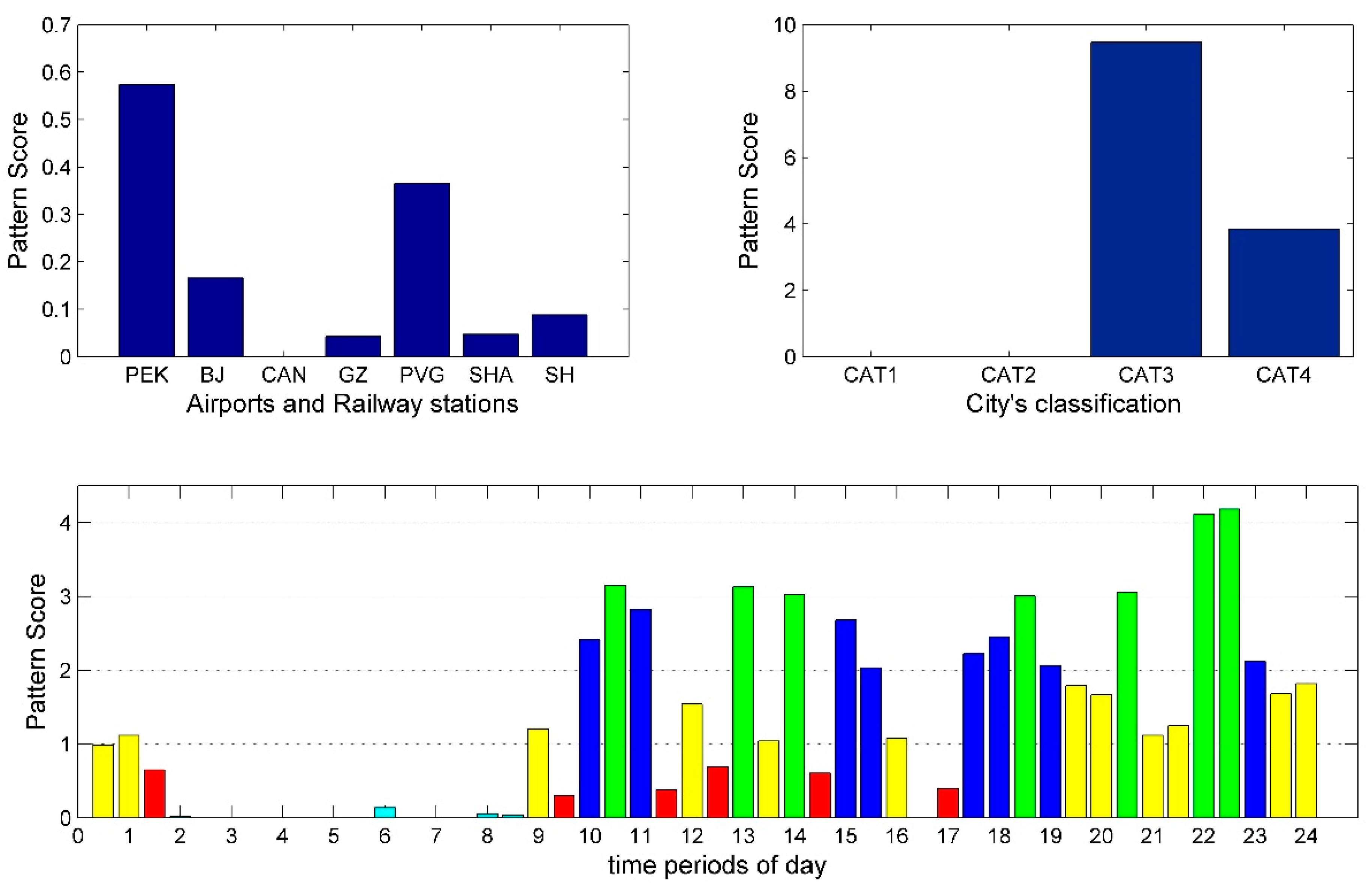
3. Patterns Recognition Result

The size of the tensors is set to 7 × 4 × 48, representing seven airport/railway stations, four classes of cities, and 48 time period of the day (half-hour period in 24 h). The number of patterns is a key parameter to be determined first. A small number of patterns does not refactor every situation, while too many will lose commonality. According to the methodology in the previous section, the number of patterns computation result is shown in Figure 1. Construct ratio, which is calculated from the relative residual between the original and approximated tensors, gradually increases, and the first turning point in Figure 1 that reaches the locally stable phase with two consecutive values was chosen as the number of patterns. The larger number of patterns not only bring better decomposition results but also more difficulties in understanding and analysis, which is a trade-off problem. Therefore, R = 7 (seven for Departure and seven for Arrival) is adopted as the specified number of potential patterns whose decomposition results can reconstruct almost 80% of the departure and arrival tensors in this study. The iterations for the departure and arrival tensors are 661 and 337, respectively.
The pattern scores, which come from the set of values of the latent factors decomposed by NTF, are presented in Figure 2, Figure 3, Figure 4, Figure 5, Figure 6, Figure 7, Figure 8, Figure 9, Figure 10, Figure 11, Figure 12, Figure 13, Figure 14 and Figure 15. The codes BJ, GZ, and SH represent the railway station of Beijing, Guangzhou, and Shanghai, respectively. The pattern score of airports and railway stations, and city’s classification indicate pattern conformity degree. The higher the score, the higher the pattern conformity degree for the corresponding airport, railway station, and city category. Furthermore, the pattern score value corresponding to the time period represents the supply level during that period. The higher the score value, the greater the supply level. Note that the fluctuation of supply level with time period, plus conformity degree of airport, railway station and city category together reflects the supply configuration pattern.
For the purpose of accurately analyzing the change in supply level over time periods, K-means was introduced to cluster the supply level pattern score, i.e., each column of the factorized matrix F 3 for different supply configuration patterns. Moreover, to facilitate the capture of supply level pattern score fluctuations, cluster separation ( SP ¯ ) is introduced, which reflects the average distance between two cluster centers. The calculation of SP ¯ is shown in Equation (3).
SP ¯ = 2 k 2 k i = 1 k j = i + 1 k w i w j 2
where k is the cluster number; w i and w j are cluster cores. SP ¯ indicates the fluctuations in the supply level of the pattern. The larger the SP ¯ value, the greater the gap between the clusters of the pattern. The clustering results are shown in Table 2. Accordingly, the supply level pattern score bars in Figure 2, Figure 3, Figure 4, Figure 5, Figure 6, Figure 7, Figure 8, Figure 9, Figure 10, Figure 11, Figure 12, Figure 13, Figure 14 and Figure 15 are marked with different colors to distinguish different clusters for each supply configuration pattern.

4. Result Analysis

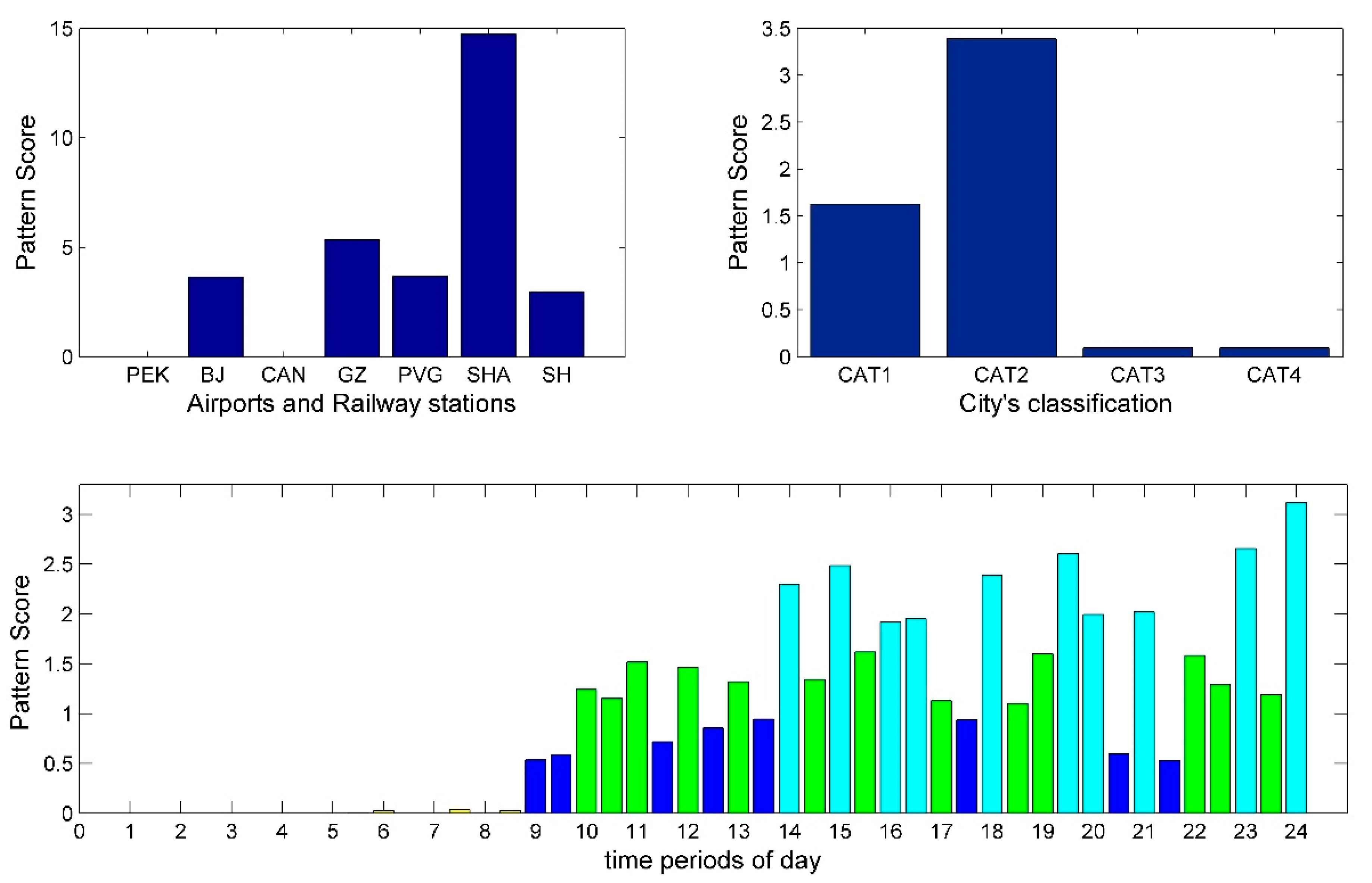
4.1. Overall Evaluation of the Pattern

Figure 2, Figure 3, Figure 4, Figure 5, Figure 6, Figure 7, Figure 8, Figure 9, Figure 10, Figure 11, Figure 12, Figure 13, Figure 14 and Figure 15 show that the pattern conformity degree of airports, railway stations, and city categories varies significantly with supply level distribution. However, it is necessary to indicate that the pattern scores are only for the pattern to which they belong. Thus, the pattern score cannot be directly compared across patterns. To comprehensively evaluate each pattern, especially to analyze its supply level peak characteristics, three indicators of peak span, average peak interval, and peak period ratio are introduced. The peak span refers to the length of time spanned by the first and last time periods of the cluster with the highest supply level in the pattern. The average peak interval (API) represents the average interval between adjacent supply level peak periods in the peak span. It reflects the degree of compactness within the peak cluster. Furthermore, the peak period ratio (PPR) represents the proportion of the number of peak periods in the total number of peak span periods. The combination of these three indicators enables a comparison of supply levels across patterns. For example, when the two patterns have the same peak span, the one with a smaller API and a higher PPR has a greater degree of supply peak aggregation. Figure 16 shows the supply level peak characteristic evaluation result of 14 patterns, where the green and blue dots represent the departure and arrival traffic respectively, and the area of the dots represents the magnitude of the PPR. The evaluation results show that there is a large difference in the peak aggregation degree of each pattern. For the API, 11 of the 14 patterns are between 0 and 5, showing a high degree of aggregation. Meanwhile, for peak span, there is a large range of variation for each pattern. Note that the API of departure pattern 6 is zero because there is only one period in the peak cluster. Moreover, the PPR of each pattern is negatively correlated with peak span and API. That is, PPR decreases as the peak span and API increase. The following sections provide a detailed analysis and comparison of each pattern on this basis.

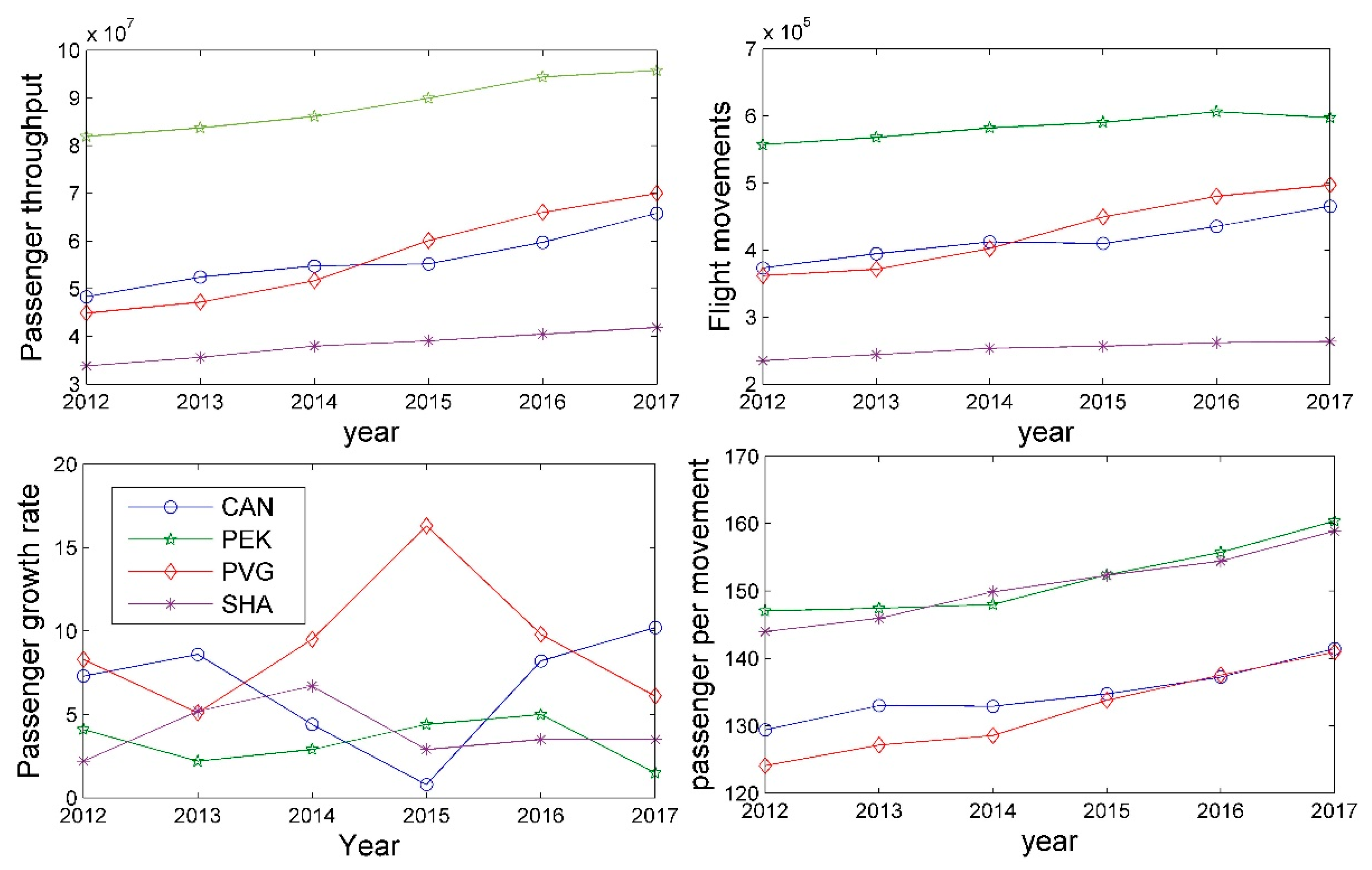
4.2. The Trend of Development of CAT1 Airports

PEK, CAN, PVG, and SHA as major hub airports in China, their development has their own characteristics. Figure 17 shows the passenger enplanements and annual growth rate, annual flight movements and passengers/movement of the CAT1 airports in the past 6 years.
PEK is the busiest airport in China. The passenger enplanement exceeded 90 million by 2017. It is the world’s second largest airport for passenger enplanement, next to Hartsfield–Jackson Atlanta International Airport. However, the passenger growth rate and flight movements have maintained a low level of growth for the last 6 years. This reveals that the PEK is in a state of saturation. The airport slot resource is very limited. To meet the needs of sustained demand growth, an increase in the average number of passengers per movement has been used by airlines at PEK. This indicator has grown rapidly since 2014. Similar situations are also observed in SHA. How to improve the utilization efficiency of slot capacity becomes the main challenge of their development.
Different from PEK and SHA, PVG and CAN show strong growth potential. Before 2014, CAN was ahead of PVG in terms of passenger enplanement, flight movements and passengers per movement. However, PVG has greatly increased the flight movements and passengers per movement at the same time since 2014, then completed the anti-overtaking against CAN in 2015. On the other side, CAN seems to prefer to achieve passenger enplanement growth by increasing the flight movements. Thus, it can be seen that the characteristics and limited conditions of the airport will make a difference in flight scheduling.

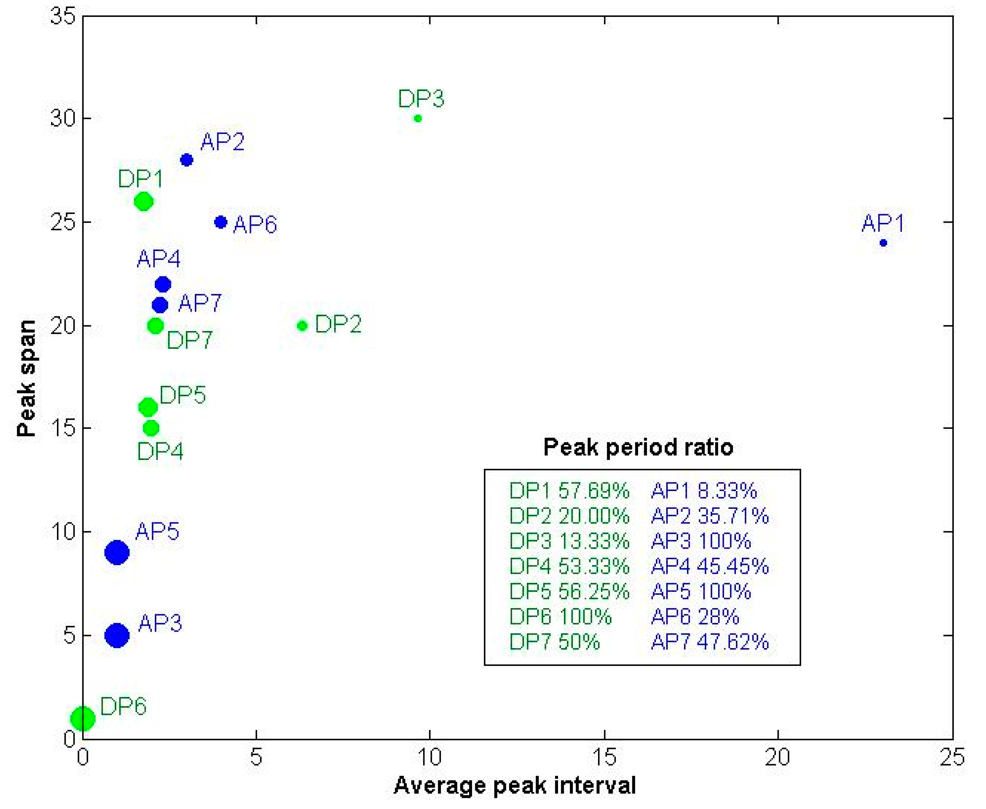
4.3. Pattern Analysis and Comparison

4.3.1. Departure Traffic

The CAT2 cities have a high conformity degree with the supply level shown in Figure 2. The scores between airports and railway stations in the same city are relatively close, except in Guangzhou (CAN and GZ). Furthermore, its peak span is from 7:30 to 20:30 with API of 1.7857 and PPR of 57.69%. The supply level of this pattern shows a high supply intensity. It also reveals that the arrangement of scheduled services of this pattern is very similar in Beijing and Shanghai. This state reflects strong competition within the scheduled services.
Cascetta E. et al. [16] adopted the maximum likelihood method to estimate desired departure time (DDT) temporal distribution for different distance classes and travel purposes from 3237 observed DDT data. Their daily DDT distribution for business travel on long distances (i.e., greater than 400 km) is presented in Figure 18. In our case, it is assumed that passengers follow the same DDT distribution. Supply peak periods shown in Figure 2 are highly correlated with the peak periods of DDT presented in Figure 18. It reveals that both railway and air transport arrange their schedules based on the same passenger departure preference to attract potential passengers as much as possible.
However, Guangzhou (CAN and GZ) seems to follow another strategy, and its flight and railway departure arrangements reflect distinct features. Figure 5 and Figure 8 correspond to the case where CAN has high conformity with CAT2 and CAT1 cities, respectively. Their peak spans are very close, CAT1 in departure pattern 7 is 2 h longer than CAT2 in departure pattern 2 in both morning and afternoon. No peak of the evening exists. Meanwhile, the optimal cluster number for departure pattern 4 and departure pattern 7 are three and five, respectively. The number of clusters represents the diversity of supply level, and the larger the number of clusters, the more supply level distributions. Furthermore, the SP ¯ of departure pattern 7 is larger than departure pattern 4. This means that the differences between clusters are greater. Compared with CAT2 cities, CAN provides more flexible supply distributions for CAT1 cities in our case. From a passenger perspective, this also means more choices and better services. Moreover, by comparing Figure 7 and Figure 8, departure supply configurations for CAT1 cities have a big difference between flight and train. Flights from CAN to CAT1 cities concentrate on 6:00 to 16:30 while railway supply level is much lower within the same period. The railway peak at GZ for CAT1 cities appears at 20:30. This is because Guangzhou is relatively far from Beijing (2146 KM) and Shanghai (1744 KM), the HSR has no advantage in travel time under these distances. The railway adopts such arrangements to avoid direct impact from flights. Therefore, this shows that transportation from Guangzhou to other CAT1 cities is mainly competition among airlines rather than the competition between flight and railway.
Furthermore, Figure 3 and Figure 4 correspond to the cases where PEK has a high conformity degree to the supply levels of CAT1 and CAT2 cities, respectively. Compared with other departure patterns, the peak span and API of these two patterns are larger while the PPR is lower. This implies that their peak supply levels are not high. However, by comparing their SP ¯ , departure pattern 2 is relatively small. It indicates that the departure pattern 2 supply level is more uniform within the peak span, while departure pattern 3 has a higher aggregation of supply level for CAT2 cities. From a convenience point of view, a uniformly distributed supply level can provide a wide range of departure time options, while supply level aggregation means that such more choices only occur at certain specific aggregation periods. Therefore, PEK provides a better departure convenience for CAT1 cities than CAT2 cities.
Similarly, BJ, SHA, and SH in Figure 6 have a higher conformity degree with CAT1 cites, with BJ being the most significant. The difference from GZ in Figure 7 is that the peak range of this pattern is 11:30 to 19:30. Considering the relatively small SP ¯ and API values, the supply level of this pattern is sufficient. It is worth pointing out that since SHA and SH are located together, the rail–air can better collaborate in this pattern from the perspective of passenger transit. However, since PEK and BJ are far apart, the characteristics of BJ in this pattern make PEK’s traffic to CAT1 face the full competition of BJ’s HSR during the day.
Overall, the conformity degree of CAT1 and CAT2 cites in different patterns are negatively correlated. Although CAT3 and CAT4 have a low conformity degree due to low supply level for the patterns, they are positively correlated. This shows that rail–air intercity transportation has different emphasis on the supply of different types of cities. The CAT1’s rail–air intercity transport has higher supply levels and better convenience than CAT2 cities, while departure time selection and service convenience to CAT3 and CAT4 cities are not as good as CAT1 and CAT2 cities from the perspective of the passenger.

4.3.2. Arrival Traffic

The arrival traffic patterns have some characteristics as the departure traffic pattern. However, it still has some differences that need to be analyzed. Figure 9 and Figure 12 correspond to the cases where PEK has a high conformity degree to the supply levels of CAT2 and CAT1 cities, respectively. Although their peak spans are similar, their PPR remain different, which is 8.33% and 45.45%, respectively. It shows that for PEK, the supply level of arrival traffic from CAT1 cities is still higher than CAT2 cities. Furthermore, Figure 14 shows PEK and PVG have a high conformity degree to the supply levels of CAT3 and CAT4 cities. The peak span of the supply level in Figure 14 is almost the same as that of the CAT1 and CAT2 cities. However, its PPR is lower than CAT1 cities but higher than CAT2 cities. In fact, this is the only pattern in which CAT3 and CAT4 cities have higher pattern conformity. This is because the airport departure capacity of CAT3 and CAT4 cities is not saturated and they can arrange the departure time slot according to their own preferences, but this leads to accumulation of arrival time slots at the destination airport. In Figure 14, the airports in addition to CAN in the CAT1 cites have this pattern conformity with CAT3 and CAT4 cities.
By comparing Figure 11 and Figure 13, the arrival supply configuration pattern of CAN for CAT1 and CAT2 cities shows a significant difference. The arrival supply level peak for CAT2 is from 19:00 to 23:30, while for CAT1 it is pushed back to 22:30 to 02:00 on the next day. Both patterns have a PPR of 100%. Thus, they have the highest supply level peak aggregation in their peak span. Compared with the airports in Beijing and Shanghai, this measure has improved the utilization of slot resources fully by staggering the arrival peak, which helps CAN increase flight movements.
Although PVG and SHA are both located in Shanghai, their arrival supply configuration patterns difference remains distinct. Figure 10 and Figure 15 show that PVG and SHA have higher pattern conformity for CAT2 cities, respectively. The PVG peak span is from 10.00 to 23:30, while SHA is from 14.00 to 24.00, and the peak supply level slowly increases with time. PPR and SP ¯ for them are 35.71% and 2.3483, 47.62% and 0.8289, respectively. This shows the supply intensity of SHA to CAT2 cities is greater than PVG. Considering that SHA and the HSR station are located together, passengers from CAT2 cities to Shanghai can get more transit convenience at SHA.
Overall, in Figure 12, Figure 14 and Figure 15, the airports and railway stations of Beijing and Shanghai have higher consistency in pattern conformity. In addition to the fact that SHA and HSR stations are located together to facilitate coordinated operation, for PEK and PVG, intercity rail–air transportation reflects more competition. Moreover, because Guangzhou is far away from Beijing and Shanghai, airlines and railways provide services according to their own advantages, and they show complementarity in the supply level.
Note that to clarify the problem, the representative patterns are selected for comparison in the analysis process, but all the possible situations are not limited to this.

4.4. Inspiration for Practical Application

Between Beijing, Shanghai, and Guangzhou, there are two of the world’s busiest networks, the air route network and the high-speed rail network. Through recognition and analysis of the intercity rail–air transport supply configuration, some inspirations and suggestions are made.
a. The peak span and supply intensity of the intercity rail–air supply configuration in Beijing, Shanghai, and Guangzhou reflect their respective characteristics depending on the departure or arrival traffic. For departure traffic, Beijing and Shanghai have supply aggregation for CAT1 and CAT2 cities due to traffic volume and priority considerations. Then for arrival traffic, CAT3 and CAT4 cities lead to supply aggregation. From the perspective of travel time selection, going to CAT3 and CAT4 cities from Beijing and Shanghai is obviously not as convenient as CAT1 and CAT2 cities, especially for departure traffic. Therefore, from the perspective of fairness and welfare, this issue deserves further improvement.
b. Whether it is a railway station or an airport, Guangzhou has differentiated supply configurations according to different city categories. This measure does not allocate the supply according to the traditional DDT, and makes full use of each time period with a specific strategy. This will enable Guangzhou to flexibly adjust the supply configuration patterns based on changes in external conditions. Moreover, Guangzhou is a unique market due to its proximity to Shenzhen and Hong Kong which provide an alternative to air and rail transport. There is a possibility of passenger leakage to these markets which has not been analyzed due to scope limitation. However, this work is worth considering in future analysis.
c. The similarity of intercity rail–air transport supply configuration patterns between Beijing and Shanghai is high at the current stage. This has created a fierce competition between aviation and railways. For travelers, it will bring more travel options and more attractive travel expenses. However, as both sides continue to increase supply capacity in this way, the overall efficiency of the system may be damaged by excessive competition. Therefore, despite the difficulties in implementation, policymakers should establish a high-level collaborative framework to guide both sides in deep cooperation between railway timetable and flight schedule planning.
d. From the perspective of providing passengers with a better travel experience, through the study of rail–air intercity traffic supply pattern recognition and peak characteristics, it can provide theoretical reference for the supply configuration of urban traffic, such as bus, subway, and taxi, especially for customized bus and ride-sharing which have emerged in recent years, to achieve efficient, comfortable and environmentally friendly travel.

5. Conclusions

This paper investigated the application of NTF to extract the supply configuration pattern of intercity rail–air transport from the constructed tensors. To compare these two different modes of transport under different city categories, supply level was proposed under the effect of decomposition and the BCD algorithm. The designed method could effectively carry out pattern recognition for the tensors of departure and arrival which have different factors including the studied airports and railway stations, the connected city’s classification, and time periods. At the same time, a good performance of the method in terms of computation speed and solution quality was observed.
The experimental results showed significant pattern characteristics and reveal the status of rail–air transport supply between different airports, railway stations, and city classification by patterns compassion. The current discussion between competition and efficiency can not only deepen our understanding of their supply configuration but also provide some new perspectives for practical policymakers when transport system efficiency and equity must be considered.
As for future work, accessing passenger flow data (demand side) and integrating it into a united patterns recognition is a meaningful extension.

Author Contributions

Conceptualization, H.Z., G.Q. and W.G.; Data curation, H.Z. and X.H.; Funding acquisition, W.G.; Methodology, H.Z. and G.Q.; Supervision, W.G.; Writing—original draft, H.Z. and X.H.; Writing—review and editing, G.Q.

Funding

This research was funded by the National Natural Science Foundation of China under Grant No.71621001 to W.G.

Conflicts of Interest

The authors declare no conflict of interest. The funders had no role in the design of the study; in the collection, analyses, or interpretation of data; in the writing of the manuscript, or in the decision to publish the results.

References

  1. Zhang, Q.; Yang, H.; Wang, Q. Impact of high-speed rail on China’s Big Three airlines. Transp. Res. Part A 2017, 98, 77–85. [Google Scholar] [CrossRef]
  2. Yang, H.; Dobruszkes, F.; Wang, J.; Dijst, M.; Witte, P. Comparing China’s urban systems in high-speed railway and airline networks. J. Transp. Geogr. 2018, 68, 233–244. [Google Scholar] [CrossRef]
  3. Jiang, C.; Zhang, A. Effects of high-speed rail and airline cooperation under hub airport capacity constraint. Transp. Res. Part B 2014, 60, 33–49. [Google Scholar] [CrossRef]
  4. Román, C.; Martín, J.C. Integration of HSR and air transport: Understanding passengers’ preferences. Transp. Res. Part E Logist. Transp. Rev. 2014, 71, 129–141. [Google Scholar] [CrossRef]
  5. Takebayashi, M. How could the collaboration between airport and high-speed rail affect the market? Transp. Res. Part A 2016, 92, 277–286. [Google Scholar] [CrossRef]
  6. Jiang, C.; Zhang, A. Airline network choice and market coverage under high-speed rail competition. Transp. Res. Part A Policy Pract. 2016, 92, 248–260. [Google Scholar] [CrossRef]
  7. Chen, Z. Impacts of high-speed rail on domestic air transportation in China. J. Transp. Geogr. 2017, 62, 184–196. [Google Scholar] [CrossRef]
  8. Lee, D.D.; Seung, H.S. Learning the parts of objects by non-negative matrix factorization. Nature 1999, 401, 788–791. [Google Scholar] [CrossRef] [PubMed]
  9. Marti-Henneberg, J. Attracting travellers to the high-speed train: A methodology for comparing potential demand between stations. J. Transp. Geogr. 2015, 42, 145–156. [Google Scholar] [CrossRef]
  10. Escobari, D. Airport, airline and departure time choice and substitution patterns: An empirical analysis. Transp. Res. Part A Policy Pract. 2017, 103, 198–210. [Google Scholar] [CrossRef] [Green Version]
  11. Ministry of Housing and Urban-Rural Development of the People’s Republic of China (MOHURD) Home Page. Available online: http://www.mohurd.gov.cn/xytj/index.html (accessed on 18 July 2018).
  12. 12306 CHINA RAILWAY Home Page. Available online: https://www.12306.cn/index/ (accessed on 21 January 2018).
  13. China Railway High-speed Home Page. Available online: http://shike.gaotie.cn/ (accessed on 21 January 2018).
  14. Kolda, T.G.; Bader, B.W. Tensor Decompositions and Applications. Siam Rev. 2009, 51, 455–500. [Google Scholar] [CrossRef] [Green Version]
  15. Carroll, J.D.; Chang, J.J. Analysis of individual differences in multidimensional scaling via an N-way generalization of Eckart-Young decomposition. Psychometrika 1970, 35, 283. [Google Scholar] [CrossRef]
  16. Harshman, R.A. Foundations of the PARAFAC procedure: Model and conditions for an “explanatory’’ multi-mode factor analysis. UCLA Work. Pap. Phon. 1970, 16, 1–84. [Google Scholar]
  17. Tucker, L.R. Some mathematical notes on 3-mode factor analysis. Psychometrika 1966, 31, 279–311. [Google Scholar] [CrossRef] [PubMed]
  18. Xu, Y.; Yin, W. A Block Coordinate Descent Method for Regularized Multiconvex Optimization with Applications to Nonnegative Tensor Factorization and Completion. Siam J. Imaging Sci. 2012, 6, 1758–1789. [Google Scholar] [CrossRef]
  19. Kolda, T.G. Multilinear Operators for Higher-Order Decompositions; Office of Scientific & Technical Information Technical Reports; OSTI: Washington, DC, USA, 2006. [Google Scholar]
  20. Fackler, P.L. Notes on Matrix Calculus. 2005. Available online: http://www4.ncsu.edu/~pfackler/ (accessed on 24 March 2019).
  21. Cascetta, E.; Coppola, P.; Rose, J. Assessment of schedule-based and frequency-based assignment models for strategic and operational planning of high-speed rail services. Transp. Res. Part A 2016, 84, 93–108. [Google Scholar] [CrossRef]
Figure 1. Number of patterns computation result. The red dot and red circle indicates the construct ratio corresponding to the different number of patterns and the selected number of patterns.
Sustainability 11 01803 g001
Figure 2. Departure pattern 1: Decomposition results of departure tensor. the supply level pattern score bars in Figure 2, Figure 3, Figure 4, Figure 5, Figure 6, Figure 7, Figure 8, Figure 9, Figure 10, Figure 11, Figure 12, Figure 13, Figure 14 and Figure 15 are marked with different colors to distinguish different clusters for each supply configuration pattern.
Sustainability 11 01803 g002
Figure 3. Departure pattern 2: Decomposition results of departure tensor.
Sustainability 11 01803 g003
Figure 4. Departure pattern 3: Decomposition results of departure tensor.
Sustainability 11 01803 g004
Figure 5. Departure pattern 4: Decomposition results of departure tensor.
Sustainability 11 01803 g005
Figure 6. Departure pattern 5: Decomposition results of departure tensor.
Sustainability 11 01803 g006
Figure 7. Departure pattern 6: Decomposition results of departure tensor.
Sustainability 11 01803 g007
Figure 8. Departure pattern 7: Decomposition results of departure tensor.
Sustainability 11 01803 g008
Figure 9. Arrival pattern 1: Decomposition results of arrival tensor.
Sustainability 11 01803 g009
Figure 10. Arrival pattern 2: Decomposition results of arrival tensor.
Sustainability 11 01803 g010
Figure 11. Arrival pattern 3: Decomposition results of arrival tensor.
Sustainability 11 01803 g011
Figure 12. Arrival pattern 4: Decomposition results of arrival tensor.
Sustainability 11 01803 g012
Figure 13. Arrival pattern 5: Decomposition results of arrival tensor.
Sustainability 11 01803 g013
Figure 14. Arrival pattern 6: Decomposition results of arrival tensor.
Sustainability 11 01803 g014
Figure 15. Arrival pattern 7: Decomposition results of arrival tensor.
Sustainability 11 01803 g015
Figure 16. Supply level peak characteristic evaluation result.
Sustainability 11 01803 g016
Figure 17. The trend of development of CAT1 airports.
Sustainability 11 01803 g017
Figure 18. The desired departure time (DDT) distribution for business travel over long distances (Cascetta E et al. [21]).
Sustainability 11 01803 g018
Table 1. City (airport) classification.
IndicatorCities (Airports)HSR Coverage Ratio
CAT1Beijing (PEK), Shanghai Pudong (PVG), Shanghai Hongqiao (SHA), Guangzhou (CAN)100%
CAT2Tianjin (TSN), Dalian (DLC), Hangzhou (HGH), Xiamen (XMN), Nanjing (NKG), Qingdao (TAO), Fuzhou (FOC), Shenzhen (SZX), Wuhan (WUH), Haikou (HAK), Changsha (CSX), Sanya (SYX), Chengdu (CTU), Kunming (KMG), Chongqing (CKG), Xi’an (XIY), Urumchi (URC), Shenyang (SHE), Harbin (HRB), Zhengzhou (CGO), Jinan (TNA), Nanning (NNG), Guiyang (KWE)100%
CAT3Nanchang (KHN), Zhuhai (ZUH), Yinchuan (INC), Taiyuan (TYN), Xining (XNN), Hohhot (HET), Changchun (CGQ), Shijiazhuang (SJW), Ningbo (NGB), Lanzhou (LHW), Hefei (HFE), Guilin (KWL), Wenzhou (WNZ)76.9%
CAT4The remaining cities (airports)21.3%
Table 2. K-means based supply level pattern score clustering results.
Pattern IDOptimal Cluster NumberSilhouette Coefficient SP ¯
Departure pattern 130.85121.8102
Departure pattern 250.84520.3108
Departure pattern 330.86588.5821
Departure pattern 430.81080.4131
Departure pattern 540.84821.1791
Departure pattern 620.989773.068
Departure pattern 750.86630.8069
Arrival pattern 150.82721.5222
Arrival pattern 220.82332.3483
Arrival pattern 320.97539.8210
Arrival pattern 450.87001.8622
Arrival pattern 530.93244.1883
Arrival pattern 650.83131.0773
Arrival pattern 740.82240.8289

