Article

How to Balance the Trade-off between Economic Development and Climate Change?

1
School of Economics and Management, Dalian University of Technology, Dalian 116024, China
2
School of Finance, Dongbei University of Finance and Economics, Dalian 116023, China
*
Author to whom correspondence should be addressed.
Sustainability 2019, 11(6), 1638; https://doi.org/10.3390/su11061638
Submission received: 21 January 2019 / Revised: 11 March 2019 / Accepted: 12 March 2019 / Published: 18 March 2019
(This article belongs to the Special Issue Climate Change and Sustainable Development Policy)

Abstract

:
Climate change is not only an environmental issue but also a development problem. Maintaining rapid economic development while simultaneously mitigating climate change is a pivotal and challenging task. Previous studies mainly focused on testing the validity of the environmental Kuznets hypothesis but ignored the internal influencing mechanism. This paper extends the past work in three aspects. First, we theoretically discuss the interaction of the scale, structure and technology effects of economic development and their impact on carbon emissions based on a classic model and the general equilibrium theory. Second, the relationship between carbon emissions and these three effects are examined by considering the quadratic term, and the interactive mechanism among them is evaluated by applying multiple mediating analysis. Due to the important role of the technology effect, we further divide it into different sources to reveal its impact on carbon emissions and discuss the rebound effect. Finally, the policy effect is considered, and the results demonstrate that the implementation of effective environmental regulations can mitigate the adverse impact of economic development on carbon emissions. Our research is an initial attempt to thoroughly explore the pathways to balance the trade-off between development and environment from the perspective of internal influencing mechanisms. The empirical results can serve as an important reference for making policies about energy conservation and emission reduction.

1. Introduction

Climate change is one of the most challenging issues faced by mankind in the 21st century, and it will bring a series of problems, such as glacial recession, extreme weather, spread of disease and collapse of the social system. According to the fifth assessment report (AR5) published by the Intergovernmental Panel on Climate Change (IPCC), as temperature has increased, the sea level has risen by 19 cm, and the future situation will be even worse [1]. Currently, greenhouse gas emissions from the combustion of fossil fuels have reached unprecedented highs. To mitigate climate change and avert further deterioration, the international community promised to cope with global warming by signing the Paris Agreement, and the contracted parties agreed to participate in mitigation actions via independent contributions.
In this context, climate change respects no national borders, and no country is immune from it, especially China, who has a long path to the goal of carbon emissions reduction. Data on greenhouse gas emissions announced by the British risk assessment company Maplecroft show that China discharges more than 6 billion tonnes of CO2 each year. As demonstrated in Figure 1, the total carbon emissions of China have been far more than the sum of Europe and America, ranking first worldwide [2]. This result is because the industrial structure of China highly depends on the secondary industry, and China has a long-standing reliance on the combustion of fossil fuels and resource consumption, which is obviously unsustainable. Faced with the dual pressure from both international and domestic societies, achieving energy conservation and emissions reduction and leading the way to low-carbon development cannot be delayed. China promised that carbon emissions would peak in 2030 and carbon intensity in 2020 would decrease by 40–45% compared with that in 2005 [3].
It is challenging to achieve that goal because it is not only an environmental problem but also a development issue. Since China’s reform and opening up, the Chinese economy has gained rapid growth. During the period of the 12th Five-Year Plan (FYP) [4], the annual GDP of China grew an average of 8%, forming a win-win situation of increasing speed and quality. After 2017, major economic indicators, such as the purchasing managers index (PMI) and industrial added value, continued to be stable and improved. It is expected that GDP per capita in 2020 will quadruple compared to that in 2000. However, as a by product of economic development, carbon emissions are closely associated with the economy. At present, China is at a critical stage in the 13th FYP period and maximizing reductions in carbon emissions while maintaining sustained and rapid economic growth seems particularly important.
The premise to solve this problem is to clarify the relationship between economic development and carbon emissions. Grossman and Krueger [5] pointed out that economic development can affect carbon emissions in three ways: scale effects, technology effects and structure effects. Firstly, the scale effect refers to the economic input. Economic growth will drive resources consumption and create additional pollution. Next, the technology effect means that economic development can promote the popularity of low-carbon and energy-saving technologies so that more capital is applied to the clean sectors. Technical progress can help companies improve the technological level and enhance energy utilization efficiency to reduce the discharge of CO2 [6]. Lastly, the structural effect indicates that economic growth can accelerate the optimization of industrial structure and energy consumption structure. In general, the evolutionary process of industrial structure is from agriculture to industry in the early industrialization stage and from secondary to tertiary industry in the post-industrialization stage. Accordingly, carbon emissions will increase first and then tend to decrease. Notably, the changing process of industrial structure can partly account for the inverted U-shape of the environmental Kuznets curve (EKC).
Based on the background above, this paper extends previous work from the following perspectives. Firstly, this paper theoretically analyses the internal influencing mechanism of economic development on carbon emissions and uses the general equilibrium theory to prove the relationship among scale effect, structure effect and technology effect proposed by Grossman and Krueger [6]. Secondly, we explore the impact of multiple mediating variables on carbon emissions, to identify crucial mediators for coordinating the conflict between economic development and carbon emissions. Based on the multiple mediating effect analysis, the direct and indirect influence of economic development on carbon emissions are discussed. Conclusions show that the technology effect plays a more important role in reducing carbon emissions in the long term because the change of industrial structure will be very slow and there is a ceiling effect. Thirdly, in view of the significance of technology, we divide it into three sources: foreign direct investment (FDI), export, and research and development (RD) input, to further discuss which type of technology plays the most crucial role in curbing carbon emissions. It is found that the independent RD is a fundamental tool to decrease carbon emissions in the long term. Fourthly, we consider the impact of environmental regulation on the influencing mechanism by adding it to the equation and we find that carbon emissions reduction policies can effectively mitigate the adverse influence of economic development on carbon emissions. Finally, cross-sectional heterogeneity is considered by using the cross-sectional dependence (CD) test [7]. Based on the cross-sectional dependence, the CIPS test [8] and Westerlund test [9] are performed to test the unit root and co-integration relationship, respectively. Overall, this paper aims to explore the deeper influencing mechanism of economic development on carbon emissions to seek the economic root of the greenhouse effect and seek effective pathways to prevent climate change. The conclusion has both practical and theoretical significance to relieve the pressure of carbon emissions reduction, balance the relationship between carbon emissions and economic development and formulate corresponding policies.
The remainder of this paper proceeds as follows: Section 2 is a literature review. Section 3 elaborates the theoretical base and model specification, and the methodology and data are presented in Section 4. Section 5 shows the empirical results, and Section 6 contains further discussion. Conclusions and policy implications are discussed in Section 7.

2. Brief Literature Review

Balancing the trade-off between economic development and climate change is a challenging task and a heated topic. This relationship is analogous to two sides of the same coin. Some scholars have explored the interaction effect by applying bidirectional causality [10,11]. For example, Appiah [12] examined the causal interdependence between energy consumption, economic growth, and CO2 emissions in Ghana from 1960 to 2015 by using the Toda–Yamamoto and Granger causality tests. Other scholars investigated the presence of the EKC relationship and whether the environmental Kuznets hypothesis (EKH) is valid by building regression equations. On the one hand, studies are based on global data or data from parts of the world. Dogan and Seker [13] analyzed the influence of real income, energy consumption, trade openness and financial development on carbon emissions in the EKC model for the top countries listed in the Renewable Energy Country Attractive Index, and the empirical results supported the existence of EKH. On the other hand, due to the heterogeneous problem, many studies have been conducted on the relationship between economic development and carbon emissions centered on single countries, such as America [14], Arabian countries [15], and Russia [16]. For China, most studies proved the presence of EKC [17,18,19], indicating that carbon emissions in China will first increase and then decrease with economic development. However, there are mixed results on EKH in the existing literature, and some scholars found no evidence for the presence of EKC [20,21]. Stern [22] presented a critical history of EKC, arguing that the EKC results had a very flimsy statistical foundation and it did not applicable for all countries. Ozturk and Acaravci [23] found that EKH at a causal framework by applying a linear logarithmic model was not valid in Turkey. Shuai et al. [24] researched carbon emissions of Shanghai, China during 1994–2009 and proved an inverted N-curve between per capita output and carbon emissions with two turning points. Ahmad et al. [25] investigated the long- and short-run relationships among carbon emissions, energy consumption and economic growth in India, and showed that the EKC was invalid in India, because the growth rate of carbon emissions was dependent on energy consumption. Antonakakis et al. [26] found that the continued process of growth aggravated the carbon emissions phenomenon, so they could not provide any evidence that developed countries would grow out of environmental pollution.
According to Grossman and Krueger [5], economic development also has technology and structure effects. Nevertheless, their influences on carbon emissions have not been confirmed, and the conclusions are not consistent. Initially, the technology effect is generally represented by technical progress, and the total factor productivity is used to measure the technical progress in a country or region. Cheng et al. [27] used dynamic spatial panel models to analyze the technical progress on carbon intensity and whether it could lead to a reduction in carbon intensity in China. Empirical results indicated that technical progress played the most important role in reducing carbon intensity. Jiao et al. [28] constructed an inter-provincial RD spillover network and measured the direct and indirect technology spillover effect. The results indicated that the direct effect had a significant inhibitory effect in the nationwide, eastern and central regions of China, except in the western region, while the indirect effect varied widely in the sub-regions. Yang and Li [29] argued that technical advance was the greatest contributor to carbon emissions mitigation and deeply discussed the rebound effect of technical advance. The results proved that a rebound effect between technology and carbon emissions existed in China and differed among regions. Zhang et al. [30] investigated the dynamic carbon emissions performance and decomposed the non-radial global Malmquist carbon emissions performance index into efficiency change and technical change indexes. The results showed that the dynamic carbon emissions performance was mainly boosted by innovation. Therefore, most studies support the reduction effect of technical progress on carbon emissions, with the exception of some opposing views. Li and Wang [31] argued that technology had relatively independent economic and environmental attributes and that technical change indeed decreased aggregate carbon dioxide emissions, but the scale and intensity effects of technical change expressed positive and negative values, respectively.
Another category of research on the effect of technology on carbon emissions is to decompose the technology effect into different sources: invention, innovation and diffusion. The former two channels can be regarded as RD activities, so the most direct source for technical progress is RD input [28]. However, for developing countries, such as China, it may be inappropriate to only consider RD. Under the circumstances of economic opening, developing countries can also achieve technical progress or even technology catch-up by introducing, imitating and absorbing the advanced experience of developed countries through international trade and foreign direct investment (FDI). On the one hand, the learning-by-exporting hypothesis argues that the export of companies can improve productivity because they are able to contact advanced technology and are exposed to more rigorous standards. On the other hand, FDI can result in technology spillover through the industry chain. Numerous studies have researched their relationship with carbon emissions.
Lee and Min [32] found a positive relationship between green RD and carbon emissions and supported that firms should organize unique resources to adopt a proactive environmental strategy. Alam et al. [33] investigated how RD investment affected the environmental performance of firms measured by energy and carbon emission intensities and found that it was able to improve the firm’s environmental performance, which was consistent with the theoretical argument of the natural resource-based view. However, Kahouli [34] held the opposite view by proving the bidirectional causality between carbon emissions and RD stocks and argued that the increase in RD stocks could negatively affect the environmental quality because the current RD stocks belonged to technologies that emit high CO2. Another source of technical progress is FDI, which can result in the pollution haven effect. Developed countries will transfer their pollution-intensity industries into developing countries due to the loose rules and regulations on the environment, so the quality of FDI can directly affect the environment of developing countries. However, high-quality FDI can also lead to technological reform and knowledge spillover to promote the technical progress of developing countries. Therefore, the influence of technical progress on carbon emissions is uncertain. Zhang and Zhang [35] examined the impacts of GDP, trade structure, exchange rate and FDI inflows on China’s carbon emissions and verified the validity of the EKC. They proved that the impacts of FDI inflows were negative, indicating the low quality of FDI in China. Baek [36] estimated the effects of FDI inflows, income and energy consumption on carbon emissions by applying panel data from five ASEAN countries, and the results showed that FDI tended to increase carbon emissions, which was in support of the pollution haven hypothesis. Omri et al. [37] investigated the causality links between carbon emissions, FDI and economic growth of 54 countries, and they proved that there was bidirectional causality between FDI inflows and carbon emissions for all panels, except Europe and North Asia. Tang and Tan [38] also examined the relationship between carbon emissions and FDI and provided evidence that there were two-way causalities between carbon emissions and FDI in Vietnam. Jalil and Feridun [39] held an opposite view that financial development in China had not taken place at the expense of environmental pollution, and on the contrary, FDI led to a decrease in environmental pollution. Finally, export can also contribute to technical progress and further affect carbon emissions with the existence of the learning-by-doing effect. Mulali and Ozturk [40] used panel non-stationary techniques to examine the effect of influencing factors on carbon emissions and the existence of the EKC hypothesis, and the results demonstrated that trade openness was able to reduce carbon emissions. Based on the above discussion, we observe that the technology effect can explicitly affect carbon emissions; however, the influencing direction and source are still uncertain.
Third, the conclusions on how the structure effect can influence carbon emissions are relatively consistent. Zhang et al. [41] discussed that upgrading the industrial structure under the constraints of CO2 emissions reduction policies was an urgent challenge for northeastern China, and empirical results proved that changing the industrial structure helped northeastern China mitigate carbon emissions. Nevertheless, more effective and targeted strategies were required for sustainable future industrial development. Shafiei and Salim [42] explored the determinants of carbon emissions for OECD countries, and the empirical results showed that the current industrial structure would increase carbon emissions. Thus, continuously optimizing the industrial structure is an effective way to control environmental pollution. Banaerjee and Rahman [43] held the same idea that there was a co-integrated relationship between industrial output growth and carbon emissions in Bangladesh, and the current industrial structure would increase carbon emissions. Zhou et al. [44] used panel data to analyze the relationship between industrial structural transformation and carbon emissions in China and found that the first-order lag of industrial structural adjustment could effectively reduce carbon emissions, while technical progress itself would not reduce emissions but indirectly cause a decrease in carbon emissions by optimizing and upgrading the industrial structure.
Although various studies have been conducted on analyzing how the scale, technology and structure effects of economic development can affect climate change, the following problems still exist: first, due to differences in data periods, research objectives and research methods, mixed results are presented, and conclusions are contradictory on how these effects can separately influence carbon emissions. Secondly, few studies focus on their interaction and the internal influencing mechanism. To the best of our knowledge, the impact of economic development on carbon emissions is complex, so analyzing the combined action of three effects on carbon emissions is meaningful. Thirdly, when discussing the existence of EKC, the policy effect is usually neglected. To address these problems, this paper will initially explore whether the EKC hypothesis exists among carbon emissions, economic growth, technical progress and industrial structure to analyze their relationships. Then, the interaction among the three effects will be illustrated by applying multiple mediating effect analysis to discuss their internal influencing mechanism on carbon emissions. Based on the results that technical progress plays a dominant role in reducing carbon emissions, we divide it into different sources to further determine what kind of technical progress can have the greatest influence on carbon emissions. Finally, the policy effect is discussed by introducing it into the EKC model to test whether the current policy is effective in energy conservation and emission reduction.
Relevant studies are summarized in Table 1.

3. Theoretical Setting and Model Specification

The earliest model with regard to carbon emissions was proposed by Grossman and Krueger [5], and they listed the decomposition equation:
E t = j = 1 n Y t ( E j t Y j t ) ( Y j t Y t ) = j = 1 n Y t I j t S j t , j = 1 , 2 , , n   ,
where t and j represent time and industry, respectively, E is the pollution emissions, Y is the gross regional domestic product, I is the emission intensity of pollutants and S is the proportion of industry output in GDP. Equation (2) is obtained by including the differential for time on both sides of Equation (1) and dividing it by Et:
E ˙ t E ˙ E = Y ˙ Y + j = 1 n e j S ˙ j S j + j = 1 n e j I ˙ j I j , j = 1 , 2 , , n   ,
where ej denotes the proportion of industrial pollution emissions of j industry in GDP. The left side of Equation (2) is total pollution emissions, while the right side of Equation (2) signifies the growth effect, industrial structure effect and energy efficiency effect in sequence. Equation (2) describes the dynamic process of pollution emissions. Based on Equation (2), we can denote carbon emissions CEjt of j industry at time t as:
C E j t = G D P t × G D P j t G D P t × E N j t G D P j t × C E j t E N j t   ,
where GDPjt/GDPt is the proportion of output of j industry in GDP of all industries at time t, represented as Sjt; ENjt/GDPjt is the energy consumption of unit output of j industry; CEjt/ENjt represent carbon emissions resulting from unit output of j industry. Energy efficiency has a direct influence on the energy consumption of unit output and related carbon emissions, so improving energy efficiency can reduce the energy consumption of unit output and carbon emissions. Therefore, (ENjt/GDPjt) × (CEjt/ENjt) can be denoted as ETjt. Equation (3) can be further transformed into:
C E j t = G D P t × S j t × E T j t   ,
where GDPt, Sjt and ETjt are the scale, structure and technology effect, respectively. According to Grossman and Krueger [5], carbon emissions will be affected by the above effects. However, the decomposition equation only presents the driving forces of carbon emissions, and it does not indicate the influencing direction.
Therefore, we will continue analyzing the influencing mechanism of the above effects on carbon emission based on the general equilibrium theory. The built model takes different types of technology into consideration. On the one hand, the model can further prove that carbon emissions are determined by scale, structure and technology effects; on the other hand, it mainly focuses on discussing the impact of heterogeneous technologies on carbon emissions. In addition, it is quite pivotal to analyze the influencing mechanism in regard to production and management, which can fully consider the macro and micro factors.
Based on the model by Copeland and Taylor [45], the general equilibrium analysis process is as follows:

3.1. Basic Assumptions

Assume that the economic system only produces two types of products: a clean product (Y) and pollution product (X). The production of X will discharge the pollutant Z, and the emissions of Z are positively correlated to the output of X. The scale returns of X and Y remain unchanged, and product X is capital-intensive with respect to product Y. The pollutant Z will have a negative external effect on other producers or customers, so the production of Z has a social cost and enterprises must pay for corresponding opportunity costs τ. In reality, τ can be regarded as the environmental tax, pollution fee or purchased discharge permission. For a company that pursues profit maximization, discharging pollutants arbitrarily is not an optimal choice; thus, the company will decide to reduce pollution emissions by using part of the resources. Use θ [ 0 , 1 ] to represent the pollution control intensity, where θ is the ratio of resources that are used to control pollution to total resources. When θ = 0, the company completely ignores pollution control, and the output at that time is the potential output F, which can also be thought of as the production ability of a company. In comparison, if the company controls the pollution by utilizing some resources θ, its actual output and pollution emissions are (1 − θ)F and Z, where X = (1 – θ)F and Z = Ψ(θ)F. Ψ(θ) is a pollution emission function of θ, and it is a decreasing function of θ. The specific form of Ψ(θ) is:
ψ ( θ ) = 1 A ( 1 θ ) 1 / α   ,
where A represents the production technology, and the parameters obey α ( 0 , 1 ) , ψ ( ) < 0 and ψ ( ) > 0 .
Assuming that two factors are necessary for producing X and Y, and capital K and labor L, the production function of X, Y and Z can be represented as:
Y = H ( K Y , L Y )
X = ( 1 θ ) F ( K X , L X )
Z = ψ ( θ ) F ( K X , L X ) ,
where KY and LY are the input of capital and labor, respectively, to produce Y and KX and LX are the input of capital and labor to produce X. The functions H( ) and F( ) both satisfy the property of constant returns to scale, so they are homogeneous functions of capital and labor.
Based on Equations (5) and (8), Z = ( 1 θ ) 1 / α F ( K X , L X ) / A , and the production function of product X is:
X = ( A Z ) α [ F ( K X , L X ) ] 1 α   ,
where product X can be regarded as the output by inputting pollution emissions Z and potential output F, and the production function has the feature of constant returns to scale. α is the proportion of pollution input in total costs.

3.2. Cost Minimization

According to the production function in Equation (9), when producing product X, company decisions for profit maximization are made by considering two separate aspects. The first is to select the appropriate ratio of capital to labor based on exogenous capital costs w and labor wage r, to make the costs cF of potential output F the smallest. The second is to select the optimal pollutant emissions Z and potential output portfolio F to make the production costs cX of unit product X the smallest under the premise that the pollutant emissions costs τ and unit potential output costs cF are given. The above decisions can be represented as follows:
c F ( w , r ) = min { r a K F + w a L F , F ( a K F , a L F ) = 1 }
c X ( τ , c F ) = min { τ A Z + c F F , ( A Z ) α F 1 α = 1 }   ,
where a K X and a L X denote the capital and labour for the unit potential output. The first-order condition of Equation (10) is that the marginal rate of technical substitution of capital and labor is equal to the ratio of capital costs r to wage w ; that is, T R S K , L = ( F / K X ) × ( F / L X ) = r / w . The optimal first-order derivative for Equation (11) is:
( 1 α ) A Z α F = c F τ   .

3.3. Pollutant Emissions

Assume that the market is perfectly competitive and that the net profit of companies is 0, then
P X X = c F F + τ Z   ,
where P X is the price of product X and Z = A Z , representing the effective pollutant emissions. Based on Equations (12) and (13), the pollutant emissions intensity e satisfies:
e Z X = α P X A τ   .
Equation (14) indicates that there is a negative relationship between pollutant emissions intensity and the technical level A and emissions costs τ , while it is positively related to the product price P X . Based on this relationship, the total pollutant emissions can be represented as Z = S ϕ X e / P X , and the economic scale is S = P X X + P Y Y . The share of output of product X in the total output is ϕ X = P X X / ( P X X + P Y Y ) ; P Y is the price of product Y . The pollutant emissions per capita z can be obtained by dividing the total labor L on both sides of Equation (14):
z = s ϕ X e / P X   ,
where s = S / L , denoting the output per capita. By substitute Equation (14) into Equation (15), we can obtain Equation (16) after taking the logarithm:
ln z = ln α + ln s ln A ln τ   .
Clearly, Equation (16) also indicates that pollutant emissions z will be determined by scale factor s , structure factor ϕ X and technical level A . This result shows not only their relationships but also the influencing direction. The scale factor and structure scale have a negative impact on pollutant emissions, while the technical factor can help reduce pollutant emissions.
Given that the industrial structure will ultimately stay in a balanced state and the technical process will be continuous and unlimited in the long term, we will mainly discuss how technical progress can influence carbon emissions. Based on the discussion of the literature, we divide technical progress into RD input, FDI and export according to different sources.
Therefore, the technical level A can be written as:
A = exp ( γ 0 + γ 1 R D + γ 2 F D I + γ 3 E X + μ )   ,
where γ 0 is the constant term, F D I is the degree of foreign direct investment, R D is the research and development level, E X is the export, γ 1 , γ 2 and γ 3 are the influencing coefficients of technical progress, and μ is the error term, μ ~ N ( 0 , σ μ 2 ) .
On the basis of the theoretical analysis, the econometric equation can be specified as:
C E i , t = ϕ 0 + ϕ 1 G P C i , t + ϕ 2 G P C i , t 2 + ϕ 3 I N S + ϕ 4 T E P i , t + ϕ 5 E C i , t + ϕ 6 U R B i , t + ε i , t   ,
where i is province of China, i = 1 , 2 , , 30 ; t represents the time series between 2001 and 2015, t = 1 , 2 , , 15 ; C E is the total carbon emissions; G P C is the economic development measured by GDP per capita; I N S is the industrial structure; T E P is the technical progress measured by total factor productivity (TFP); Based on the literature [46,47,48,49,50,51] and practical situations of China, E C and U R B are selected as control variables, representing the total energy consumption and urbanization, respectively; and ε i , t is the random disturbance term.

4. Methodology and Data

4.1. Estimation Method

To estimate Equation (18), the fully modified ordinary least squares (FMOLS) proposed by Phillips and Hansen [52] and the dynamic ordinary least squares (DOLS) proposed by Stock and Watson [53] were used. FMOLS is able to address the estimation bias caused by the system disturbance by introducing the correction factor. Based on the OLS estimation, FMOLS can correct the balancing error and the explained variable by using nonparametric kernel estimation to eliminate the endogeneity and the serial correlation of the error term. In comparison, DOLS can solve the endogeneity of regression variables and the possible serial correlation simultaneously by applying the differential variable in the leading and lagged form of the explanatory variable. Kao and Chiang [47] compared the OLS, FMOLS and DOLS in terms of finite sample features, and the results of a Monte Carlo simulation experiment indicated that compared to the OLS estimator with inconsistent characteristics and non-negligible bias, the FMOLS and DOLS estimators with asymptotic normal distributions are better choices. However, in comparison, the FMOLS estimator cannot improve the OLS estimator significantly; instead, it will result in deviation that may even exceed the OLS estimator, especially for the homogeneous panel data. Thus, DOLS is the best estimated technique among the three methods, and it can also solve the endogenous problem well.
According to the principle of DOLS, Equation (18) can be simplified and written as:
Y i , t = a i + β X i , t + e i , t   ,
where β is the coefficient matrix, representing the co-integration coefficients; X is an independent variable and Y represents the dependent variable. Then, we introduce the leading and lagged differential variable Δ X i , t k of the explanatory variable to Equation (19):
Y i , t = a i + β X i , t + k = K i K i γ i , k Δ X i , t k + e i , t   .
According to Equation (20), β can be denoted as β ^ G D = N 1 i = 1 N ( t = 1 T Z i , t Z i , t ) 1 ( t = 1 T Z i , t Y i , t ) ; Z i , t = ( X i , t X ¯ i , Δ X i , t k , , Δ X i , t + k ) is the regression vector of 2 ( K + 1 ) × 1 , Y ˜ i , t = Y i , t Y ¯ i . Thus, the DOLS estimator can be restated as β ^ G D = N 1 i = 1 N β ^ D i , where β ^ D i is the traditional DOLS estimator of the i-th panel unit.
In addition, due to the existence of EKH, the dissimilation needs to be considered when estimating the EKC. Initially, we included the cubic term of GDP per capita into the equation to examine whether there is an N-shaped or inverted N-shaped relationship. However, the estimated results were not significant, so we did not list the results and only discussed the quadratic term of GDP per capita.

4.2. Tests before Model Construction

4.2.1. Cross-Sectional Dependence Test

Because the variable or residual correction across panel members due to the global common shocks and the spillover effect can lead to inaccurate estimation of the model, Pesaran [54] proposed the cross-sectional dependence (CD) test to verify whether a cross-sectional correlation exists. This test has the following hypotheses:
H0: 
No cross-sectional dependence.
H1: 
Existence of cross-sectional dependence.
The CD test is robust in the presence of multiple breaks in error variance and in slope coefficients.
Assume that the panel data model to be estimated is described in Equation (21), and when the cross-section N is larger than time T, the CD statistic can be calculated by Equation (22):
y i t = α i + β i x i t + u i t , i = 1 , 2 , , N , t = 1 , 2 , , T
C D = T N ( N 1 ) ( i = 1 N 1 j = i + 1 N ρ ^ i j )   ,
where α i and β i are the intercept term and slope of the sample regression equation, respectively; u i t is the residual term; and ρ ^ i j is the covariance between the residual term of each cross section after the ordinary least squares.

4.2.2. Panel Unit Root Test

The second issue to be addressed before model estimation was to examine the existence of a panel unit root. According to the co-integration theory, all variables should be integrated with first order, I(1). Although the literature on unit root tests is abundant, most panel unit root tests, such as the LLC test [55], HT test [56], Breitung test [57], IPS test [58], Fisher-type test [59,60] and Hadri test [61], were performed under the assumption of cross-sectional independence in the dynamics of the autoregressive coefficients. Considering the cross-sectional dependence, Pesaran [7] proposed the cross-sectionally augmented IPS panel unit root test (CIPS) to avoid the presence of spatial spillover, the omission of common factors and the residual interdependence among other factors. CIPS can be calculated by:
C I P S = N 1 i = 1 N C A D F i   ,
where C A D F i represents the individual cross-sectionally augmented Dickey–Fuller statistic for individual i or time series [54].

4.2.3. Panel Co-Integration Test

The third issue to be solved was determining whether there is a long-term co-integration relationship between variables. The non-stationary variables should have a stationary linear combination. Similar to the panel unit root test, the panel co-integration tests should consider the cross-sectional dependence. Usually, the Kao test [62] and Pedroni test [63] are suitable for cross-sectional independence problems, while the Westerlund test [9] can be performed when assuming cross-sectional dependence.
In this paper, in light of the presence of cross-sectional dependence, the Westerlund test based on the panel error-correction model is employed as described in Equation (24):
Δ y i t = δ i d t + α i ( y i , t 1 β i x i , t 1 ) + j = 1 p i α i j Δ y i , t j + j = q i p i γ i j Δ x i , t j + e i t , i = 1 , 2 , , N , t = 1 , 2 , , T ,
where T is the time series and N is the number of provinces, respectively; d t is the deterministic factor, and when d t = 0 , there is no deterministic factor; when d t = 1 , Δ y i t contains the constant term; and when d t = ( 1 , t ) , Δ y i t contains both the constant term and the trend term; x i t is the k-dimension random walk sequence, and Δ x i t and e i t are independent variables; α i is the speed to return to the balanced state y i , t 1 β i x i , t 1 after the short-term impact. When α i < 0 , there is an error-correction term and y i t and x i t have a co-integration relationship; conversely, when α i = 0 , there is an error-correction term or co-integration relationship. Therefore, the null hypothesis of the Westerlund test is H 0 : α i = 0 for all provinces i; accordingly, the alternative hypothesis is to ensure that α i is homogeneous, and it can be divided into two groups: group-mean tests ( G T , G α ) and panel tests ( p T , p α ). For the former group, the α i value of each cross section does not need to be equal, so the alternative hypothesis can be that H 1 g : α i = 0 for at least one i; the latter group assumes that the α i value of each cross section is equal, so its alternative hypothesis is H 1 p : α i = α < 0 for all i. The four statistic are shown in Equations (25) and (26):
{ G T = 1 N i = 1 N α ^ i S E ( α ^ i ) G α = 1 N i = 1 N T α ^ i α ^ i ( l )
{ P T = α ^ i S E ( α ^ ) P α = T α ^   ,
where S E ( α ^ i ) is the standard error of α ^ i ; α ^ i ( l ) is calculated by the variance estimator of the long-term co-integration equation of Newey and West [64]; α ^ = ( i = 1 N t = 2 T y ˜ i , t 1 2 ) 1 i = 1 N t = 2 T 1 / ( α ^ i ( 1 ) ) y ˜ i , t 1 Δ y ˜ i t .

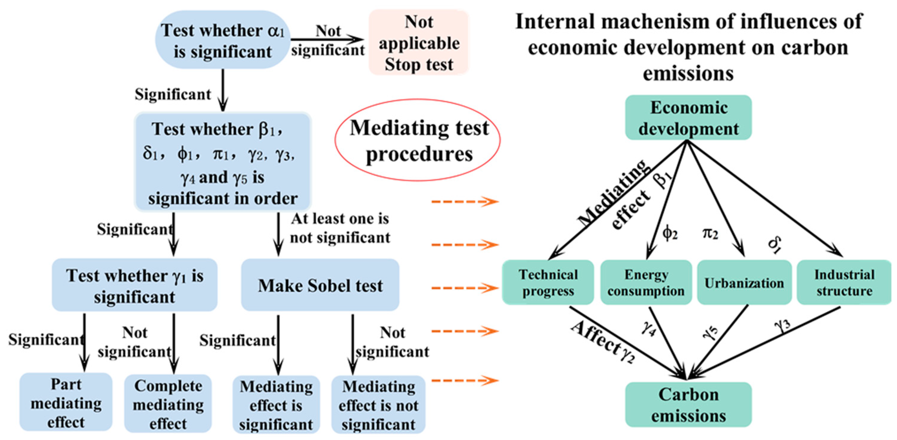
4.3. Multiple Mediating Effect Analysis

To further study the interactive mechanism of the scale, structure and technical factors, the multiple mediating effect model is applied to test the direct and indirect impact of economic development on carbon emissions. It is assumed that economic development will directly affect carbon emissions through scale effect and indirectly affect carbon emissions through technology and structure effects. The equations of the multiple mediating effect model are as follows:
C E i , t = α 0 + α 1 G D P i , t + ε i , t
T E P i , t = β 0 + β 1 G D P i , t + ε i , t
I N S i , t = δ 0 + δ 1 G D P i , t + ε i , t
E C i , t = ϕ 0 + ϕ 1 G D P i , t + ε i , t
U R B i , t = π 0 + π 1 G D P i , t + ε i , t
C E i , t = γ 0 + γ 1 G D P i , t + γ 2 T E P i , t + γ 3 I N S i , t + γ 4 E C i , t + γ 5 U R B i , t + ε i , t   .
To verify the presence of a mediating effect, three steps can be followed, as shown in Figure 2:
Step 1. Estimate Equation (27) to examine whether the coefficient of economic development, α 1 , is significant. If it is significant, economic development can affect carbon emissions; move to Step 2. If not, stop the test.
Step 2. Estimate Equation (28), Equation (29), Equation (30) and Equation (31) to test the significance of the coefficient of technical progress, industrial structure, energy consumption and urbanization. If β 1 , δ 1 , ϕ 1 and π 1 are all significant, perform Step 3.
Step 3. Estimate Equation (32) to determine the existence of a mediating effect. If γ 2 , γ 3 . γ 4 and γ 5 are all significant and γ 1 is smaller than α 1 , there is a partial mediating effect. If γ 1 is not significant but γ 2 , γ 3 . γ 4 and γ 5 are significant, the four variables play the complete mediating role.

4.4. Data and Variables

Considering the availability of data, we choose to research 30 provinces in China during 2001-2015. The core variables include carbon emissions, economic growth, technical progress, RD input, FDI, export and industrial structure, and the control variables are energy consumption and urbanization. The measurement, economic implications, explanation and sources are described below and shown in Table 2. For carbon emissions and technical progress, the detailed calculation process is described as follows:
Carbon emissions mainly come from two sources: combustion of fossil fuels and production of cement. For the former source, coal, oil and natural gas are the most widely applied fossil fuels, accounting for 66%, 17.1% and 5.7% of the total energy consumption, respectively. Therefore, this paper chooses 13 types of related fossil fuels, including raw coal, cleaned coal, other washed coal, briquettes, coke, crude oil, gasoline, kerosene, diesel oil, fuel oil, liquefied petroleum gas, refinery gas and natural gas, to calculate the cumulative carbon emissions to improve the accuracy. Equation (33) shows the detailed equation:
C f o s s i l = j = 1 13 C i t j = j = 1 13 M i t j × K j × q j   ,
where M i t j is the physical quantity of the j-th fossil fuel in the i-th province in the t-th year; K j is the standard coal efficiency collected from the China Energy Statistical Yearbook [65]; and q j is the carbon emissions coefficient, which was published by the Intergovernmental Panel on Climate Change (IPCC) in 2006 [1]. K j and q j are constants because utilization efficiency of carbon emissions remains unchanged in the short term. Secondly, carbon emissions generated from the cement production process can be calculated by Equation (34):
C c e m e n t = N i t × a   ,
where N i t is the physical quantity of cement in the i-th province in the t-th year and a is the carbon emissions factor with a value of 0.5272 [66]. Data on cement output in each province of China can be collected from the CEinet Statistics Database [67].
Technical progress is reflected by total factor productivity (TFP) and was calculated based on data envelopment analysis (DEA) and the Malmquist index. According to the principle of DEA–Malmquist, each province can be regarded as a decision-making unit (DMU), and the TFP of 30 provinces in China can be measured to reflect the generalized technical progress. ( x t , y t ) denotes the input and output at the t-th time. The production technology can be defined as Equation (35), and the output distance function of the production possibility set is shown as Equation (36):
F t = { ( x t , y t ) :   all   x t   can   be   used   to   produce   y t }
D t ( x t , y t ) = inf { φ > 0 : ( x t , y t / φ ) F t }
where D represents the distance; φ is the technical efficiency; inf is the greatest lower bound; and F is the production possibility frontier. Equation (36) can reflect the reciprocal of magnification of output y with fixed input x at the technical level in the t-th period. When the input-output combination is at the production technical frontier, D t ( x t , y t ) = 1 . Thus, the Malmquist index can be constructed as Equation (37):
M 0 ( x t , y t , x t + 1 , y t + 1 ) = D 0 t + 1 ( x t + 1 , y t + 1 ) D 0 t + 1 ( x t , y t ) × [ D 0 t + 1 ( x t + 1 , y t + 1 ) D 0 t + 1 ( x t + 1 , y t + 1 ) × D 0 t ( x t , y t ) D 0 t + 1 ( x t , y t ) ] 1 2 = E F F C H × T E P C H   .
The key to calculating the DEA–Malmquist index is to choose proper input and output indexes. In this paper, capital stock and labor force were the input indexes, and GDP is the output index. We estimate the capital stock by applying the perpetual inventory method according to Shan [68]. The labor force is represented by the average value of the labor force at the beginning and end of the year. Related data are all from the China Statistical Yearbook [69].

5. Empirical Results

5.1. Results of the Tests Before Analysis

Prior to panel unit root tests, we perform the CD test, considering that the variable or residual correction across panel members can lead to the problem of inaccurate estimates of models due to the global common shocks and spillover effect. The results in Table 3 show that each variable under consideration rejects the null hypothesis that there is no cross-sectional relationship. On the other hand, the correlation coefficient that measures the degree of cross-sectional dependence is high, further proving the cross-sectional dependence of the variables.
When a cross-sectional dependence is present, we use the CIPS test to conduct the panel unit root test. Table 4 demonstrates that variables in levels with or without a trend all accept the null hypothesis of the existence of a panel unit root; however, when using the first-order difference of each variable, the null hypothesis is rejected. Therefore, we conclude that all variables examined obey the I(1) process.
After confirming the I(1) process of each variable, the final issue to be solved is to test whether there is a co-integration relationship by the Westerlund test allowing for cross-sectional dependence. Table 5 reveals that the robust p-value of Ga, Pt and Pa was 0.000, rejecting the null hypothesis that there is no co-integration. Therefore, a long-term equilibrium exists between the two variables, which is a pivotal premise for the subsequent analysis.

5.2. Impact of Each Effect on Carbon Emissions

The influences of scale, technology and structure effects on carbon emissions are shown in Table 6. The results of FMOLS and DOLS were almost similar from the perspectives of sign, magnitude and statistical significance, verifying the robustness of the estimated results. As discussed above, DOLS can obtain more reliable results, so the following analysis is based on the results of DOLS. Model (5) presented the basic regression results of three variables without quadratic items. At the 5% significance level, GPC, INS and EC all negatively affected carbon emissions, while TEP and URB had a positive impact on carbon emissions. EC had the greatest influence, followed by GPC, INS, TEP and URB. The quadratic items of GPC, INS and TEP were separately introduced into model (6)–(8), and the results demonstrated that GPC and TEP both had an inverted U-shape relationship with carbon emissions, but the relation between INS and carbon emissions tends to be linear. The values of R-square and adjusted R-square of models (5)–(8) were all above 0.800, indicating a good fit. The detailed analysis of the influences of each variable on carbon emissions is as follows:
(1)
Economic development. The negative impact of economic development on carbon emissions shows that the current economic development in China can contribute to increasing carbon emissions. Then, by adding the quadratic term of GPC into the equation, the presence of EKH was tested. In fact, we also considered the cubic term of GPC, but it was not significant, so we do not show the related results for simplicity. The coefficients of GPC and GPC square were 0.492 and −0.351, respectively, proving the existence of EKH and an inverted U-shape between carbon emissions and economic development. Our research results are consistent with those reported by [35,49]. It is confirmed that early-stage development in China negatively impacts the environment, especially during the industrialization and urbanization processes. Currently, although China is becoming better by promoting industrial transformation from the secondary industry to the tertiary industry and developing morelow-carbon technologies, much work is still needed for China to balance economic development and environmental pollution.
(2)
Industrial structure. According to model (7), INS negatively affected carbon emissions, while its quadratic item was not significant even at the 10% significance level. When the proportion of the secondary industry increases by one unit in GPC, carbon emissions will increase by 0.159 units. The results indicate that the continuous increase in the output value of the secondary industry will damage the environment without any turning point, which has critical implications for carbon emissions reduction. On the one hand, a large number of energy-intensive industries with heavy emissions and consumption, such as the thermal power industry and manufacturing industry, are included in the secondary industry. Therefore, to control carbon emissions, it is imperative to achieve low-carbon development of the secondary industry. On the other hand, industrial transformation is priority number one, and each country, especially China, is seeking to update and develop their industry towards a green industry. At present, China still depends on the secondary industry. For example, despite the rapid development of renewable energy, thermal power plays the dominant role in China in supplying electricity. In addition, from a perspective of the global value chain, the advantages of China center on the manufacturing industry. Thus, to control carbon emissions, China should positively promote an industrial transformation from the traditional secondary industry to the modern service industry and high-tech industry.
(3)
Technical progress. The impact of TEP on carbon emissions was positive, indicating that technical progress can help reduce carbon emissions. Furthermore, the results in Table 6 show that there is an inverted U-shape relationship between carbon emissions and technical progress. When the technology is at an initial stage, it will cause an increase in carbon emissions because, at that time, the development of technology will be at the expense of the environment. After arriving at a certain threshold, technical progress can contribute to a decrease in carbon emissions. Currently, China’s technology is developing at a high speed, including carbon capture and storage technology for traditional energy and some renewable energy technologies. Therefore, stimulating technical progress is the most essential and effective way to rapidly improve environmental quality and mitigate climate change in both the short and long run. In the Paris Agreement, China has promised that by 2030, carbon emissions will peak, and the Chinese government will undertake to implement the carbon intensity reduction of 60–65% below 2005 level by 2030 [72]. According to model (8), when carbon emissions reach the peak, the technical progress will be 0.625, which is high. We did not estimate the relationship between technical progress and carbon intensity of China, but based on the results in Table 6, it can be known that when technical progress increases 1 unit, carbon emissions will decrease by 0.229 units. Therefore, to achieve that goal, technical progress will be very high. Although technical progress can be used as a tool, it needs to undergo great changes. To promote the rapid development of technical progress and accelerate the carbon emissions reduction, stringent environmental regulation will be needed for a deep decarbonization.
(4)
Control variables. Compared with the three major driving forces, energy consumption had the largest impact on carbon emissions, indicating that energy consumption is the main source of carbon emissions. However, energy consumption is incorporated into economic development, industrial structure updating and technical progress, and those processes will all consume energy. Our results are also consistent with the research conducted by [73,74]. The energy can be divided into two types: renewable energy and non-renewable energy. The former is clean and sustainable, including wind and solar, while the latter, such as coal and oil, generates pollutants. The energy consumption examined in this paper indicates the total energy consumption, so the negative impact means that the energy consumption structure of China still overwhelmingly relies on non-renewable energy. The resources in China consist of abundant coals, minor oil and no gas, and the proportion of coal consumption to the total energy consumption is above 60%. Specifically, the thermal power industry, which can generate approximately 80% of China’s cumulative electric power, undoubtedly belongs to the coal-consumption sector. Until now, the installed capacity of thermal power has remained high, with a proportion above 74%. Therefore, our estimated results are meaningful for China to make policies to reduce carbon emissions. China should vigorously explore and develop renewable energies to gradually replace non-renewable energy. Another control variable is urbanization. Based on the DOLS results, at the 5% significance level, urbanization can significantly reduce carbon emissions, and this inhibiting effect becomes more obvious with the continuous promotion of the urbanization process. Our conclusion is proven by Yao et al. [51], who also argued that urbanization could present an abatement effect on carbon emissions, but such an abatement effect would be diminished with increasing urbanization. However, due to the different research data and methods applied, Wu et al. [75] reached the opposite conclusion. In recent years, the rapid development of urbanization has effectively improved the clustered benefits and economic-scale effects of population, traffic and industry, dramatically promoting resource conservation and driving the development of the service industry, such as catering, tourism, modern logistics and the financing and banking industry. Therefore, carbon emissions can be reduced. The results have great practical significance because, according to previous researches, urbanization is a contributor to the rise of carbon emissions. However, currently, the situation is different and more optimistic, and carbon emissions can be controlled by accelerating the urbanization process.

5.3. Interaction Among the Three Effects on Carbon Emissions

After clarifying the role of the scale, structure, and technology effects separately, their interactions were discussed by applying the multiple mediating effect analysis. Here, technical progress, industrial structure, energy consumption and urbanization were considered to be mediating variables between economic development and carbon emissions. The scale effect was regarded as a direct effect, while the structure and technology effects were regarded as indirect effects. From Table 7, it can be seen that the regression coefficients of GPC, TEP and EN were all significant, and the coefficient of GPC in model (14) is 0.386, which is smaller than that in model (9), with a value of 0.414. The detailed analysis is as follows:
1) Individual mediating effect. The mediating effect of technical progress was −0.5112, which is significant at the 1% significance level. This result means that technical progress can mitigate the scale effect of increasing GPC. Similarly, the mediating effect of energy consumption is −0.6921, so the energy consumption can increase carbon emissions. The mediating effect of the other two variables are not obvious.
2) Overall mediating effect. This effect can be obtained by calculating the individual mediating effect, and the value is 1.2003. The direct effect of economic development on carbon emissions was 0.2331, indicating that after removing the mediating effect of technical progress and energy consumption, economic development will not contribute to carbon emissions reduction; instead, it will contribute to an increase in carbon emissions. Therefore, we can conclude that promoting technical progress is an importantly functional mechanism for decreasing carbon emissions.
3) Comparison of individual mediating effects. According to the previous analysis, the individual mediating effects of technical progress and energy consumption on carbon emissions were −0.5112 and −0.6921, respectively, accounting for 42.6% and 57.4% of the overall mediating effect. The mediating effect of technical progress was nearly half in terms of absolute values and proportions in the overall mediating effect. Therefore, compared to industrial structure, technical progress is more effective in controlling carbon emissions and can effectively reduce the adverse impact of energy consumption and economic development on carbon emissions.
The results of the mediating effect analysis show that promoting technical progress is the most important channel to reduce carbon emissions, and without the above two mediating variables, the scale effect of economic development will lead to an increase in carbon emissions. Moreover, the effect of technical progress on reducing carbon emissions was more significant, and it is the main channel to decrease carbon emissions. On the one hand, the technical progress signifies that the technical level of each industry should be improved, which can prominently control carbon emissions. For example, for a long time, coal-fired power generation has been the dominant energy source in China; thus, the focus should not replace coals with other types of energy but instead develop low-carbon technologies, such as carbon capture and storage and desulfurization technology, which are more aligned with the current situations in China. On the other hand, the popularity and speed of technology is faster than the industrial adjustment speed. Industrial transformation is a slow process, and China will still depend on primary energy, such as coals. In addition, technical progress can be regarded as unlimited and completed in a few years, while the transformation of industrial structure is a slow process, and even the industrial sector is changed from secondary to tertiary, the problem of carbon emissions will still exist. So, the potential of the structure effect is restrictive. Therefore, promoting technical progress is a key method to reduce carbon emissions in the short and long term.

5.4. Discussion of Technology Effect

In view of the significance of the technology effect in easing carbon emissions, this section mainly discusses how technical progress can affect carbon emissions by dividing it into different sources. The equation is as follows:
C E i , t = ϕ 0 + ϕ 1 G P C i , t + ϕ 2 G P C i , t 2 + ϕ 3 I N S + ϕ 4 R D i , t + ϕ 5 F D I i , t + ϕ 6 E X i , t + ϕ 7 E C i , t + ϕ 8 U R B i , t + ε i , t   ,
where RD is research and development, representing the technical progress within China; FDI is foreign direct investment, denoting the technology spillover, and it can measure whether the FDI of China is of high quality; EX is the export, which can test whether the learning-by-doing hypothesis exists.
The results in Table 8 show the technology effect based on DOLS. In this case, there is still an inverted U-shape between carbon emissions and economic development, with a positive coefficient for GPC and a negative coefficient for GPC2. Similar to the above results, INS and EC can cause an increase in carbon emissions, while URB can lead to a decrease in carbon emissions. Then, we will focus on analysing the three technology effects. Firstly, the influence of RD is positive, which indicates that independent research and development in China has become a main source of technical progress. With rapid development, China has possessed many advanced technologies, especially in the field of energy conservation and emission reduction. This result implies that the most important and sustainable method to control carbon emissions is to enhance the ability of national independent RD. Second, FDI has a significantly negative impact on carbon emissions at the 5% significance level. This result proves the existence of the pollution haven effect and implies that China needs to improve the quality of FDI and focus more on the introduction of green FDI. On the other hand, FDI is not a source of technical progress, nor does it contribute to carbon emissions reduction. This is because that the environmental regulations in China are relatively loose, and many international companies regard China as a trade factory that produces products with high carbon emissions. The international trade and FDI focus more on the energy-intensive industry, and both the products themselves and the process to produce products contain high carbon emissions. The research results are also supported by [31]. Finally, the coefficient of EX is negative, indicating that it can mitigate carbon emissions. Thus, the learning-by-doing hypothesis exists in China, and technical progress is achieved during the export process. Exporters will strengthen the innovation ability among the fierce export competition, which has a positive impact on improving the technical level.

6. Further Discussion

6.1. Discussion on Policy Effect

Faced with the increasingly serious problem of carbon emissions, the Chinese government has attached great importance to this problem and proposed that China’s carbon intensity will be reduced by 40–45% in 2020 and 60–65% in 2030. Since 1979, China has begun to impose a blowdown fee and enacted many regulations and policies to decrease environmental pollution and carbon emissions. However, whether energy or environmental policies can effectively accelerate carbon emissions reduction is still controversial. On the one hand, Wang et al. [17] argued that energy policies play a consistent role in regulating carbon emissions. Zhang et al. [76] considered that the clean development mechanism (CDM) was beneficial for the development of renewable energy and reduction of carbon emissions. On the other hand, the research by Zhang et al. [41] showed that the impact of the Central Rise Policy of China on carbon emissions at the stage of operation in road sectors proved relatively weak during 2006–2015. Similarly, Peng [77] used the investment in industrial pollution control as the proxy variable of environmental regulation and confirmed that the influence of environmental regulation on carbon emissions reduction was not obvious. The mixed nature of the empirical findings investigated above proves that it is significant to continue exploring this issue and determine whether environmental regulation can affect the relationship between economic development and carbon emissions.
In this section, we will examine the policy effect by answering the question: Can the negative impact of the scale effect on carbon emissions be reduced when considering environmental regulation? To solve this problem, we introduced a variable, named the environmental regulation level, to reflect the policy effect. This variable can be measured by the ratio of total investments on industrial pollution control to the industrial added value. The equation to be tested is:
C E i , t = θ 0 + θ 1 I P C i , t + θ 2 G P C i , t + θ 3 G P C i , t 2 + θ 4 I P C i , t × G P C i , t + θ 5 I N S i , t + θ 6 E C i , t + θ 7 F D I i , t + θ 8 R D i , t + θ 9 E X i , t + θ 10 U R B i , t + ε i , t
where IPC represents the environmental regulation level. The higher the value is, the higher the environmental regulation level is; conversely, the lower the value is, the lower the environmental regulation level is.
The results in Table 9 demonstrate an interesting conclusion that the coefficient of IPC and its interaction term with GPC is significant, and the inverted U-shape still exits. But the influencing amplitude of GPC on carbon emissions is smaller compared with results without IPC. This result has two implications: 1) Although economic development can affect carbon emissions and the EKC exists, the policy to control carbon emissions can diminish such impact. In addition, the negative coefficient of the interaction term between IPC and GPC shows that when the investment of industrial pollution control increases, the influence of GPC decreases. 2) When considering IPC, the impact of export, FDI and urbanization becomes insignificant. Therefore, we can further infer that the policy plays a very pivotal role in reducing carbon emissions because it not only weakens the impact of economic development but also reduces the effect of the pollution haven effect; therefore, the government should focus full attention on the environmental problems and formulate effective policies to control carbon emissions.

6.2. Discussion on Rebound Effect

In this paper, we focus on discussing how technical progress can contribute to carbon emissions reduction; however, it might be not true that technical progress is always able to decrease carbon emissions. Technical progress will boost the economic growth as well, which is at the cost of using more fossil fuel energies to replace labor force and capital investment in the production activities [29]. This phenomenon is called as rebound effect (RE), and it can directly influence the ultimate impact of technical progress on carbon emissions reduction. Therefore, although the vital influence of technical progress on reducing carbon emissions has been proven above, the rebound effect cannot be ignored, and should be discussed. In this section, we initially analyze reasons for the rebound effect, and then calculate the rebound effect of China.
According to Equation (25), TEPCH and EFFCH represents the technical changes and efficiency changes of TEP, respectively. As shown in Table 10, coefficients of TEP and EFFCH are both negative, indicating that they can contribute to carbon emissions reduction; however, what is interesting is that the coefficient of TEPCH is positive, and it means that technical changes will increase carbon emissions. In general, technical innovation is of three types: original innovation, integrated innovation, and digestion, absorption and re-innovation. Technical changes always result from original innovation, while efficiency changes are caused by the latter sources. That is, the efficiency changes will affect the economic system through secondary innovation, which can shorten the distance between technical frontier and economic system [27]. In comparison, innovation related to efficiency change is more mature and can promote the utilization of available energy and reduce carbon emissions effectively. So, the results further prove the existence of rebound effect, and it is improper to conclude that technical progress can curb carbon emissions at no costs.
The rebound effect will be calculated by applying the method of Yang and Li [29]. The carbon emissions rebound effect at the macro level is defined as Equation (40) (please refer to [29] for specific steps to deduce Equation (40)).
R t = A t × Y t × C I t + 1 Y t + 1 × ( C I t + 1 C I t ) × γ t = ( T E P C H t t + 1 1 ) × Y t × C I t + 1 Y t + 1 × ( C I t + 1 C I t ) × ( Δ C I i t p / Δ C I t )   ,
where T E P C H t t + 1 is the technical changes extracted from TEP from time t to time t + 1; Y t is the economic output, which is measured by GDP; C I t + 1 and C I t are carbon intensity at time t + 1 and t, which is the ratio of carbon emissions to GDP. In the method of Yang and Li [29], they used LMDI method to decompose the carbon intensity and defined that the changes of carbon intensity ( Δ C I t ) were caused by changes of energy structure ( Δ C I i e s ), industrial structure ( Δ C I i i s ) and technical progress ( Δ C I i t p ). Based on Equation (40), the rebound effect of China from 2002–2015 can be estimated.
Table 11 presents estimated results of carbon emissions rebound effect. The results are basically consistent with the results of Yang and Li [29]. We update the data from 2011–2015 and our results are a bit larger than their results due to differences of samples selection and data processing methods. In addition to the year of 2005, when the rebound effect was negative, other years had positive rebound effects. It indicates that before 2005, China has invested more money in promoting economic growth instead of carbon emissions reduction or energy savings. After that, the rebound effect becomes positive. Since 2011, the rebound effect has become smaller, and the declining tendency reflects that the policies for carbon emissions reduction of Chinese government are effective to some extent and such effectiveness increases stably. On the other hand, technical progress is not the only means to curb carbon emissions, and it needs to coordinate with other policies, such as environmental regulation and carbon tax. However, compared with results of Zhang et al. [27], our estimated rebound effect is much smaller, because we followed the methods of Yang and Li [29] and used LMDI to decompose carbon intensity into different components. So, it results in the distinct results. In this paper, we consider that decomposing the carbon intensity is more reasonable, for it can differentiate changes of carbon emissions caused by technical progress with other sources.

6.3. Robust Test

To prove the robustness of the estimated results, several additional tests are performed by considering two aspects: estimating methods and variables. First, as shown in Table 6, the direction of the variables, amplitude of coefficients and significance are almost similar for the two methods of DOLS and FMOLS, which further proves that our estimated results can successfully avoid the bias caused by using only one estimation method. Second, one may argue that the indicator of total carbon emissions is not representative, so we repeat our analysis with alternative indicators: carbon emissions per capita. In addition, the variable exports are replaced with imports for a robust test. The estimated results show that the relevant variables lost their statistical significance but never changed the direction of influence. Therefore, the variation in the variables does not change the main findings. For simplicity, we do not list the results of the robustness tests.

7. Conclusions and Policy Implications

This paper studies how to balance the trade-off between economic development and carbon emissions by discussing the interaction among scale, technology and structure effects. The conclusions are rich and interesting, and the main findings are summarized as follows:
(1)
Economic development and industrial structure will both negatively affect carbon emissions, while technical progress has a positive influence on carbon emissions. An inverted U-shape exists among carbon emissions, economic growth and technical progress, but the relationship between industrial structure and carbon emissions is linear. Our results confirm that there is a threshold point for economic growth and technical progress, and carbon emissions will increase first and then decrease after the threshold value.
(2)
As for the interaction among the scale, technology and structure effects, economic development can increase carbon emissions directly through the scale effect and indirectly decrease carbon emissions through the technology effect. Therefore, promoting technical progress and optimizing the industrial structure are two effective ways to mitigate carbon emissions. In comparison, the technical progress is unlimited and can play a key role in the short and long terms, while the role of the industrial structure is less important because it is a slow process to update it.
(3)
In view of the importance of promoting technical progress, to realize the goal of China in the Paris Agreement, technical progress needs to be fast. However, it will be not possible for technical progress to be so high in the short run. So stringent environmental regulation will be needed for deep decarbonization. To further explore the impact of technical progress, we divide it into different sources: RD, FDI and export. The empirical results prove that the most direct technical progress in China is national RD, so investing more into RD in China can help achieve the promise of reducing carbon emissions. Both the pollution haven hypothesis and learning-by-doing hypothesis exist in China. On the one hand, the quality of FDI should be enhanced by transforming the type of FDI from energy intensity into knowledge intensity. On the other hand, China is supposed to insist on high-quality exports and improve the environment by learning from practice. In addition, to reflect the influences of technical progress, the carbon emissions rebound effect is calculated and discussed. The existence of rebound effect is proven, and it is between 12% and 62% during 2001–2015. Results indicate that the technical progress alone cannot achieve the necessary carbon emissions reduction and too much focus on technical solutions might lead to a dead end. So other policies should coordinate with technical progress.
(4)
By considering the policy effect, we obtain that the policies related to energy savings and emissions reduction can have a great impact on controlling carbon emissions. When there are effective policies, the impact of economic development on carbon emissions becomes much smaller. Additionally, the negative influence of other variables becomes less significant as pollution control strengthens.
Based on the conclusions above, some recommendations are proposed:
First, to promote the technical progress is a fundamental strategy for China to reduce carbon emissions. Compared with other industries, it is urgent to improve the technical level in the secondary industry. One of the important conclusions of this paper is that there is no a turning point for the industrial structure in China, and it fully indicates that the current development of manufacturing industry is at the cost of sacrificing the environment. For example, the main source of carbon emissions in China is energy consumption in thermal power industry, because it highly depends on the coal-fired generation due to natural resource conditions of China. Therefore, enhancing the technical level in the power generation sector can help reduce carbon emissions greatly, such as ultra-supercritical thermal power units and coal desulfurization technology. Additionally, the manufacturing industry should continue achieving green and intelligent development. For example, it is useful to accelerate the commercial application of new-energy vehicles, smart grids and communication equipment so that the industry can be updated and transformed from extensive growth to intensive growth.
Secondly, for different sources of technology, various policies should be implemented. Initially, more investments should be used to encourage the independent RD in low-carbon technologies. Although China takes its place in the front ranks of the world in the aspect of solar and wind energy, the international competitiveness needs to be enhanced. There is still a large gap between China and other countries in patents and licensing of low-carbon technologies. So, China should stimulate enterprises to carry out innovation activities by combining production, teaching and research. In addition, to perfect the support services mechanism of technical innovation and educate high-end talents is also effective measures to strengthen the ability of RD. As for the trade, China should provide more financial and policy supports to enhance the competitiveness of products. Moreover, it is important to improve the access threshold of FDI by formulating more rigorous technical standard, industrial standard and environmental standard. In the eastern inshore area, most foreign companies engage in processing trade business, and currently, some high-carbon industries have not been put into the category of prohibited industry; therefore, it is suggested that the Chinese government put them in the prohibited category to control carbon emissions from the source.
Finally, it is known that the policy effect is important for controlling carbon emissions; however, the existing environmental policies are still loose. So, China should improve the pollution criteria of carbon emissions, and involve the carbon emissions and environmental pollution as an indicator to measure the development of one region. In addition, the environmental regulation should also take regional differences into full consideration. By seizing the opportunity of One Belt and One Road, regions with better economic development should positively drive the development of undeveloped regions to improve the utilization rate of energy, promote capital flow and achieve win-win and harmonious results among different regions.
Notably, economic development is currently the main task for China, but economic development itself cannot control the increase or decrease of carbon emissions. Instead, it will reduce carbon emissions by the technology effect. Therefore, when formulating carbon emission reduction policies, the interaction among scale, technology and structure effects should be comprehensively considered instead of regarding economic development as the opposite side of carbon emissions. At present, China is on the front line of carbon emissions reduction, so to enforce the Paris Agreement and contribute to the global carbon emissions target, China has much work to complete.

Author Contributions

Conceptualization, X.M. and Q.J.; methodology, X.M.; software, X.M.; validation, X.M. and Q.J.; formal analysis, Q.J.; investigation, Q.J.; resources, Q.J.; data curation, Q.J.; writing—original draft preparation, X.M.; writing—review and editing, Q.J.; visualization, X.M.; supervision, X.M.; project administration, X.M.; funding acquisition, X.M.

Funding

This research was funded by the National Statistical Science Research Project, grant number 2018609; Research Foundation for Talented Scholar of Dalian University of Technology, grant number DUT18RC(3)053; Humanities and Social Sciences Research Project of the Ministry of Education, grant number 18YJC910013.

Conflicts of Interest

The authors declare no conflict of interest.

References

  1. IPCC (Intergovernmental Panel on Climate Change). The Fifth Assessment Report. 2009. Available online: http://www.ipcc.ch/report/ar5/ (accessed on 4 March 2018).
  2. Wu, Y.; Chau, K.W.; Lu, W.S.; Shen, L.Y.; Shuai, C.Y.; Chen, J.D. Decoupling relationship between economic output and carbon emission in the Chinese construction industry. Environ. Impact Assess. Rev. 2018, 71, 60–69. [Google Scholar] [CrossRef]
  3. Huang, G.X.; Ouyang, X.L.; Yao, X. Dynamics of China’s regional carbon emissions under gradient economic development mode. Ecol. Indic. 2015, 51, 197–204. [Google Scholar] [CrossRef]
  4. Gu, A.; Teng, F.; Lv, Z.Q. Exploring the nexus between water saving and energy conservation: Insights from industry sector during the 12th Five-Year Plan period in China. Renew. Sustain. Energy Rev. 2016, 59, 28–38. [Google Scholar] [CrossRef]
  5. Grossman, G.M.; Krueger, A.B. Environmental Impacts of the North American Free Trade Agreement; Working Paper 3914; NBER: Cambridge, UK, 1991. [Google Scholar]
  6. Yang, L.; Yao, Y.; Zhang, J.; Zhang, X.; Mcalinden, K.J. A CGE analysis of carbon market impact on CO2 emission reduction in China: A technology-led approach. Nat. Hazards 2016, 81, 1107–1128. [Google Scholar] [CrossRef]
  7. Pesaran, M.H. General diagnostic tests for cross section dependence in panels. Soc. Sci. Electron. Publ. 2004, 7, 1240. [Google Scholar]
  8. Pedroni, P. Panel cointegration: Asymptotic and finite sample properties of pooled time series tests with an application to the ppp hypothesis: New results. Econ. Theory 2004, 20, 597–627. [Google Scholar] [CrossRef]
  9. Westerlund, J. Testing for error correction in panel data. Oxf. Bull. Econ. Stat. 2007, 69, 709–748. [Google Scholar] [CrossRef]
  10. Esso, L.J.; Keho, Y. Energy consumption, economic growth and carbon emissions: Cointegration and causality evidence from selected African countries. Energy 2016, 114, 492–497. [Google Scholar] [CrossRef]
  11. Mirza, F.M.; Kanwal, A. Energy consumption carbon emissions and economic growth in Pakistan: Dynamic causality analysis. Renew. Sustain. Energy Rev. 2017, 72, 1233–1240. [Google Scholar] [CrossRef]
  12. Appiah, M.O. Investigating the multivariate Granger causality between energy consumption, economic growth and CO2 emissions in China. Energy Policy 2018, 112, 198–208. [Google Scholar] [CrossRef]
  13. Dogan, E.; Seker, F. The influence of real output, renewable and non-renewable energy, trade and financial development on carbon emissions in the top renewable energy countries. Renew. Sustain. Energy Rev. 2016, 60, 1074–1085. [Google Scholar] [CrossRef]
  14. Apergis, A.; Christou, C.; Gupta, R. Are there environmental Kuznets Curves for US state-level CO2 emissions? Renew. Sustain. Energy Rev. 2017, 69, 551–558. [Google Scholar] [CrossRef]
  15. Samargandi, N. Sector value addition, technology and CO2 emissions in Saudi Arabia. Renew. Sustain. Energy Rev. 2017, 78, 868–877. [Google Scholar] [CrossRef]
  16. Yang, X.C.; Lou, F.; Sun, M.X.; Wang, R.Q.; Wang, Y.T. Study of the relationship between greenhouse gas emissions and the economic growth of Russia based on the environment Kuznets Curve. Appl. Energy 2017, 193, 162–173. [Google Scholar] [CrossRef]
  17. Wang, Y.; Zhang, C.; Lu, A.T.; Li, L.; Zhu, X.D. A disaggregated analysis of the environmental Kuznets curve for industrial CO2 emissions in China. Appl. Energy 2017, 190, 172–180. [Google Scholar] [CrossRef]
  18. Wang, S.J.; Liu, X.P. China’s city-level energy-related CO2 emissions: Spatiotemporal patterns and driving forces. Appl. Energy 2017, 200, 204–214. [Google Scholar] [CrossRef]
  19. Alam, M.M.; Murad, M.W.; Noman, A.H.M.; Ozturk, I. Relationships among carbon emissions, economic growth, energy consumption and population growth: Testing environmental Kuznets Curve hypothesis for Brazil, China, India and Indonesia. Ecol. Indic. 2016, 70, 466–479. [Google Scholar] [CrossRef]
  20. Ozokcu, S.; Ozdemir, O. Economic growth, energy, and environmental Kuznets curve. Renew. Sustain. Energy Rev. 2017, 72, 639–647. [Google Scholar] [CrossRef]
  21. Zhui, H.M.; Duan, L.J.; Guo, Y.W.; Yu, K.M. The effects of FDI, economic growth and energy consumption on carbon emissions in ASEAN-5: Evidence from panel quantile regression. Econ. Modell. 2016, 58, 237–248. [Google Scholar] [CrossRef]
  22. Stern, D. The rise and fall of the environmental Kuznets curve. World Dev. 2004, 32, 1419–1439. [Google Scholar] [CrossRef]
  23. Ozturk, I.; Acaravci, A. CO2 emissions, energy consumption and economic growth in Turkey. Renew. Sustain. Energy Rev. 2010, 14, 3220–3225. [Google Scholar] [CrossRef]
  24. Shuai, S.; Yang, L.; Yu, M.; Yu, M. Estimation, chracteristics, and determinants of energy-related industrial CO2 emissions in Shanghai (China), 1994–2009. Energy Policy 2011, 39, 6476–6494. [Google Scholar]
  25. Ahmad, A.; Zhao, Y.H.; Shahbaz, M.; Bano, S.; Zhang, Z.; Wang, S.; Liu, Y. Carbon emissions, energy consumption and economic growth: An aggregate and disaggregate analysis of the Indian economcy. Energy Policy 2016, 96, 131–143. [Google Scholar] [CrossRef]
  26. Antonakakis, N.; Chatziantoniou, I.; Filis, G. Energy consumption, CO2 emissions, and economic growth: An ethical dilemma. Renew. Sustain. Energy Rev. 2017, 68, 808–824. [Google Scholar] [CrossRef]
  27. Cheng, Z.H.; Li, L.S.; Liu, J. Industrial structure, technical progress and carbon intensity in China’s provinces. Renew. Sustain. Energy Rev. 2018, 81, 2935–2946. [Google Scholar] [CrossRef]
  28. Jiao, J.L.; Jiang, G.L.; Yang, R.R. Impact of R&D technology spillovers on carbon emissions between China’s regions. Struct. Chang. Econ. Dyn. 2018, 47, 35–45. [Google Scholar]
  29. Yang, L.S.; Li, Z. Technology advance and the carbon dioxide emission in China-Empirical research based on the rebound effect. Energy Policy 2017, 101, 150–161. [Google Scholar] [CrossRef]
  30. Zhang, N.; Wang, B.; Liu, Z. Carbon emissions dynamics, efficiency gains, and technological innovation in China’s industrial sectors. Energy 2016, 99, 10–19. [Google Scholar] [CrossRef]
  31. Li, M.Q.; Wang, Q. Will technology advances alleviate climate change? Dual effects of technology change on aggregate carbon dioxide emissions. Energy Sustain. Dev. 2017, 41, 61–68. [Google Scholar] [CrossRef]
  32. Lee, K.H.; Min, B. Green R&D for eco-innovation and its impact on carbon emissions and firm performance. J. Clean. Prod. 2015, 108, 534–542. [Google Scholar]
  33. Alam, M.S.; Atif, M.; Chi, C.C.; Soytas, U. Does corporate R&D investment affect firm environmental performance? Evidence from G-6 countries. Energy Econ. 2019, 78, 401–411. [Google Scholar]
  34. Kahouli, B. The causality link between energy electricity consumption, CO2 emissions, R&D stocks and economic growth in Mediterranean countries. Energy 2018, 145, 388–399. [Google Scholar]
  35. Zhang, Y.; Zhang, S.F. The impacts of GDP, trade structure, exchange rate and FDI inflows on China’s carbon emissions. Energy Policy 2018, 120, 347–353. [Google Scholar] [CrossRef]
  36. Baek, J. A new look at the FDI-income-energy-environment nexus: Dynamic panel data analysis of ASEAN. Energy Policy 2016, 91, 22–27. [Google Scholar] [CrossRef]
  37. Omri, A.; Nguyen, D.K.; Rault, C. Causal interactions between CO2 emissions, FDI, and economic growth: Evidence from dynamic simultaneous-equation models. Econ. Modell. 2014, 42, 382–389. [Google Scholar] [CrossRef]
  38. Tang, C.F.; Tan, B.W. The impact of energy consumption, income and foreign direct investment on carbon emissions in Vietnam. Energy 2015, 79, 447–454. [Google Scholar] [CrossRef]
  39. Jalil, A.; Feridun, M. The impact of growth, energy and financial development on the environment in China: A cointegration analysis. Energy Econ. 2011, 33, 284–291. [Google Scholar] [CrossRef]
  40. Mulali, U.A.; Ozturk, I. The investigation of environmental Kuznets curve hypothesis in the advanced economies: The role of energy prices. Renew. Sustain. Energy Rev. 2016, 54, 1622–1631. [Google Scholar] [CrossRef]
  41. Zhang, Y.J.; Liu, Z.; Zhou, S.M.; Qin, C.X.; Zhang, H. The impact of China’s Central Rise policy on carbon emissions at the stage of operation in road sector. Econ. Modell. 2018, 71, 159–173. [Google Scholar] [CrossRef]
  42. Shafiei, S.; Salim, R.A. Non-renewable and renewable energy consumption and CO2 emissions in OECD countries: A comparative analysis. Energy Policy 2014, 66, 547–556. [Google Scholar] [CrossRef]
  43. Banaerjee, P.K.; Rahman, M. Some determinants of CO2 emissions in Bangladesh. Int. J. Green Econ. 2012, 2, 205–215. [Google Scholar] [CrossRef]
  44. Zhou, X.Y.; Zhang, J.; Li, J.P. Industrial structural transformation and carbon dioxide emissions in China. Energy Policy 2013, 57, 43–51. [Google Scholar] [CrossRef]
  45. Copeland, B.R.; Taylor, M.S. North-south trade and the environment. Q. J. Econ. 1994, 109, 755–787. [Google Scholar] [CrossRef]
  46. Dong, K.Y.; Sun, R.J.; Dong, X.C. CO2 emissions, natural gas and renewables, economic growth: Assessing the evidence from China. Sci. Total Environ. 2018, 640, 293–302. [Google Scholar] [CrossRef] [PubMed]
  47. Kao, C.; Chiang, M.H.; Chen, B. International R&D spillovers: An application of estimation and inference in panel cointegration. Oxf. Bull. Econ. Stat. 1999, 61, 691–709. [Google Scholar]
  48. Naves, R.B.; Pino, J.F.; Mayor, M. Do countries influence neighbouring pollution? A spatial analysis of the EKC for CO2 emissions. Energy Policy 2018, 123, 266–279. [Google Scholar] [CrossRef]
  49. Riti, J.S.; Song, D.Y.; Shu, Y.; Kamah, M. Decoupling CO2 emission and economic growth in China: Is there consistency in estimation results in analyzing environmental Kuznets curve? J. Clean. Prod. 2017, 166, 1448–1461. [Google Scholar] [CrossRef]
  50. Xu, Q.; Dong, Y.X.; Yang, R. Urbanization impact on carbon emissions in the Pearl River Delta region: Kuznets curve relationships. J. Clean. Prod. 2018, 180, 514–523. [Google Scholar] [CrossRef]
  51. Yao, X.L.; Kou, D.; Shao, S.; Li, X.; Wang, W.; Zhang, C. Can urbanization process and carbon emissions abatement be harmonious? New evidence from China. Environ. Impact Assess. Rev. 2018, 71, 70–83. [Google Scholar] [CrossRef]
  52. Phillips, P.C.B.; Hansen, B.E. Statistical inference in instrumental variables regression with I(1) processes. Rev. Econ. Stud. 1990, 57, 99–125. [Google Scholar] [CrossRef]
  53. Stock, J.H.; Watson, M.W. A simple estimator of cointegration vectors in high order integrated systems. Econometrica 1993, 61, 783–820. [Google Scholar] [CrossRef]
  54. Pesaran, M.H. A simple panel unit root test in the presence of cross section dependence. J. Appl. Econom. 2007, 22, 265–312. [Google Scholar] [CrossRef]
  55. Levin, A.; Lin, C.F.; Chu, C.S.J. Unit root test in panel data: Asymptotic and finite-sample properties. J. Econom. 2002, 108, 1–24. [Google Scholar] [CrossRef]
  56. Harris, R.D.F.; Tzavalis, E. Inference for unit roots in dynamic panels where the time dimension is fixed. J. Econom. 1991, 91, 201–226. [Google Scholar] [CrossRef]
  57. Breitung, J. The Local Power of Some Unit Root Tests for Panel Data, Advances in Econometrics, Nonstationary Panels, Panel Cointegration, and Dynamic Panels; JAI Press: Amsterdam, The Netherlands, 2000; pp. 161–178. [Google Scholar]
  58. Im, K.S.; Pesaran, M.H.; Shin, Y. Testing for unit roots in heterogeneous panels. J. Econom. 2003, 115, 53–74. [Google Scholar] [CrossRef]
  59. Maddala, G.S.; Wu, S. A comparative study of unit root tests with panel data and a new simple test. Oxf. Bull. Econ. Stat. 1999, 61, 631–652. [Google Scholar] [CrossRef]
  60. Choi, I. Unit root tests for panel data. J. Int. Money Financ. 2001, 20, 249–272. [Google Scholar] [CrossRef]
  61. Hadri, K. Testing for stationarity in heterogeneous panel data. J. Econom. 2000, 3, 148–161. [Google Scholar] [CrossRef]
  62. Kao, C. Spurious regression and residual-based tests for cointegration in panel data. J. Econom. 1999, 90, 1–44. [Google Scholar] [CrossRef]
  63. Pedroni, P. Critical values for cointegration tests in heterogeneous panels with multiple regressors. Oxf. Bull. Econ. Stat. 1999, 61, 653–670. [Google Scholar] [CrossRef]
  64. Newey, W.K.; West, K.D. Automatic lag selection in covariance matrix estimation. Rev. Econ. Stud. 1994, 61, 631–653. [Google Scholar] [CrossRef]
  65. CESY (China Energy Statistical Yearbook), 2002–2016; China Statistical Publishing House: Beijing, China, 2017.
  66. Li, K.; Qi, S.Z. Trade openness, economic growth and carbon dioxide emission in China. J. Econ. Res. 2011, 11, 60–72. [Google Scholar]
  67. CEinet Statistics Database, Cement Data. Available online: http://db.cei.gov.cn (accessed on 8 May 2018).
  68. Shan, H.J. Re-estimate of China’s capital stock K. Quantitative %. Techn. Econ. 2008, 10, 17–31. [Google Scholar]
  69. CSY (China Statistical Yearbook), 2002–2016; China Statistical Publishing House: Beijing, China, 2017.
  70. CSYFA (China Statistical Yearbook of Fixed Asset), 2002–2016; China Statistical Publishing House: Beijing, China, 2017.
  71. CDESY (China’s Demographic and Employment Statistical Yearbook), 2002–2016; China Statistical Publishing House: Beijing, China, 2017.
  72. Chen, C.; Zhao, T.; Yuan, R.; Kong, Y.C. A spatial-temporal decomposition analysis of China’s carbon intensity from the economic perspective. J. Clean. Prod. 2019, 215, 557–569. [Google Scholar] [CrossRef]
  73. Hanif, I. Impact of fossil fuels energy consumption, energy policies and urban sprawl on carbon emissions in East Asia and the Pacific: A panel investigation. Energy Strategy Rev. 2018, 21, 16–24. [Google Scholar] [CrossRef]
  74. Rahman, M.M.; Kashem, M.A. Carbon emissions, energy consumption and industrial growth in Bangladesh: Empirical evidence from ARDL cointegration and Granger causality analysis. Energy Policy. 2017, 110, 600–608. [Google Scholar] [CrossRef]
  75. Wu, Y.Z.; Shen, J.H.; Zhang, X.L.; Skitmore, M.; Lu, W.S. The impact of urbanization on carbon emissions in developing countries: A Chinese study based on the U-Kaya method. J. Clean. Prod. 2017, 163, s284–s298. [Google Scholar] [CrossRef]
  76. Zhang, Y.J.; Sun, Y.F.; Huang, J.L. Energy efficiency, carbon emission performance, and technology gaps: Evidence from CDM project investment. Energy Policy 2018, 115, 119–130. [Google Scholar] [CrossRef]
  77. Peng, S.J.; Zhang, W.C. Carbon emissions tendency of China’s household consumption and its influencing factors. World Econ. 2013, 3, 124–142. (In Chinese) [Google Scholar]
Figure 1. Carbon emissions of world main economies in 2016.
Sustainability 11 01638 g001
Figure 2. Procedure of the mediating test model and internal influencing mechanism of economic development on carbon emissions.
Sustainability 11 01638 g002
Table 1. Summary of relevant studies.
DateRegionEquationDriving ForcesRef.
1971–201012 African countries Δ Y t = μ + β i Δ Y t i + β i Δ C O 2 t j + α 1 Y t i + α 2 C O 2 t j + ε 1 , t GPC (+)[10]
1971–2009Pakistan Δ C O 2 t = α 3 + j = 1 p β 3 j Δ G D P t j + j = 1 p γ 3 j Δ E t j + j = 1 p θ 3 j Δ C O 2 t j + λ 3 E C T t 1 + μ 3 t EC (+), GPC (+)[11]
1985–201123 countries ( C O 2 ) i t = β 0 + β 1 Y i t + β 2 Y i t 2 + β 3 R E C i t + β 4 N R E C i t + β 5 T R i t + e i t GPC (+), TOP (−), EC (+/−) [13]
1980–2010OECD ln ( C O 2 ) i t = β 1 i + β 2 ln ( G D P ) i t + β 3 ( ln G D P ) i t 2 + β 4 ( ln G D P ) i t 3 + β 5 ( ln e c ) i t + u i t GPC (−), EC (+) [20]
1981–2011ASEAN Q y i t ( τ | α i , ξ t , x i t ) = α i + ξ t + β 1 τ E N C i t + β 2 τ G D P i t + β 3 τ G D P i t 2 + β 4 τ P O P i t + β 5 τ T R A D E i t + β 6 τ I N S i t + β 7 τ F D I i t + β 8 τ F I N i t EC (+), GPC (+), INS (+), FDI (−), EX (−), POP (+)[21]
2000-2013China ln C E i j t = α i + β 1 ln A i t + β 2 ( ln A i t ) 2 + β 3 ln E I i t + β 4 ln U R i t + T t + ε i t EC (+), GPC (+), URB (+)[17]
1992–2013China y i t = α y i , t 1 + β Z i t + η i + ε i t GPC (+), INS (+), POP (+), CIN (+), FDI (−)[19]
1970–2012China ln C O 2 t = β 0 + β 1 ln G D P t + β 2 ln G D P t 2 + β 3 ln E U t + β 4 ln P O P t + ε t EC (+), GPC (+), POP (+)[19]
1971–2013India L C O 2 t = α 0 + β 1 L E C t + β 2 L Y t + β 3 L Y t 2 + e t EC (+), GPC (+)[25]
1998–2014China ln C E i t = β 0 + β 1 ln Y i t + β 2 ln I S U i t + β 3 ln I S O i t + β 4 ln T F P i t + β 5 ln F D I i t + β 6 ln U L i t + β 7 ln E C S i t + ε i t EC (+), GPC (-), INS (−), TEP (−), FDI (+), URB (+) [27]
2000–2015China ln C i t = α 0 + α 1 ln D S i t + α 2 ln I S i t ( c , e , b ) + α 3 ln R S i t + α 4 ln F D I i t + α 5 ln Y i t + α 6 ( ln Y i t ) 2 + α 7 ln S i t + ε i t GPC (+), INS (+), TEP (−), FDI (−)[28]
1997–2010China R t = [ ( T E C H t t + 1 1 ) × Y t × C I t + 1 ] / [ Y t + 1 × ( C I t + 1 C I t ) × ( Δ C I i t C I i ) ] TEP (−)[29]
1990–2012China N G M C P I = [ T C P I G ( K t + 1 , L t + 1 , E t + 1 , Y t + 1 , C t + 1 ) ] / [ T C P I G ( K t , L t , E t , Y t , C t ) ] TEP (−)[30]
1996–200795 countries Δ I = I t + 1 I t = ( E t + 1 / Y t + 1 ) ( E t / Y t ) TEP (+/−)[31]
2001–2010Japanese Y i t = c o n s tan t + β 1 G R D i t + β 2 R D i t + β 3 G R D R D i t + ε i t RD (−)[32]
2004–2016G-6 countries Y i t = α + β 1 ( R D ) i t + β 2 ( G F C D ) i t + δ 3 ( f i r m ) i t + δ 4 ( i n d u s t r y ) i t + δ 5 ( y e a r ) i t + δ 6 ( c o u n t r y ) i t + ε i t RD (−)[33]
1990–2016Mediterranean countries ln C O 2 i t = α 0 + α 1 ln G D P i t + α 2 ln E E C i t + α 3 ln R D S i t + α 4 ln T i t + α 5 ln F D i t + α 6 ln P O P i t + ε i t GPC (+), RD (+), POP (−)[34]
1982–2016China L n C O 2 t = α 0 + α 1 L n Y t + α 2 L n Y t 2 + α 3 L n E I M t + α 4 L n e x t + α 5 L n F D I t + ε t GPC (+), EX (−), FDI (+)[35]
1981–2010ASEAN C O i t = α 0 + α 1 y i t + α 2 y i t 2 + α 3 e n i t + α 4 f d i i t + u i t EC (+), FDI (+)[36]
1990–201154 countries Y / L = b λ e ε A ( K / L ) α ( C O 2 / L ) λ ( F D I / L ) ψ GPC (+), FDI (+), EX (+), URB (−)[37]
1976–2009Vietnam ln C O 2 t = β 0 + β 1 ln G D P t + β 2 ln G D P t 2 + β 3 ln E C t + β 4 ln F D I t + ε t GPC (+), FDI (−)[38]
1953–2006China c t = β 0 + β 1 e t + β 2 y t + β 3 y t 2 + β 4 f d t + β 5 t r t + ε t EC (+), GPC (+), FDI (-), EX (+)[39]
1990–201227 advanced economies Δ L C O 2 i t = π 1 t + p π 11 i p L C O 2 i t p + p π 12 i p L G D P i t p + p π 18 i p L P C i t p + ε 2 i t EC (+/−), GPC (+), EX (−), URB (+)[40]
1980–2011OECD ln ( C O 2 i t ) = ln b 0 + b 1 ln ( P i t ) + b 2 ln ( A i t ) + b 3 ln ( I N D i t ) + b 4 ln ( S i t ) + b 5 ln ( U i t ) + b 6 ln ( P D i t ) + ln e 2 i t EC (+/−), GPC (+), INS (+), URB (+)[42]
1990–2012China ln C i t = β 0 + β 1 T i t + β 2 T l i t + β 3 M i t + β 4 M T i t + β 5 M T l i t + + β 11 G o v i t + β 12 I n f r a i t + β 13 U r b a n i t + γ y e a r + ε i t GPC (+), INS (−), URB (+)[44]
Note: 1) + means the positive impact; while—indicates the negative impact; 2) GPC: GDP per capita; CIN: capital investment; EC: energy consumption; TOP: trade openness; INS: industrial structure; EX: export; POP: population; URB: urbanization; TEP: technical progress; RD: research and development input.
Table 2. List and description of variables.
NameTypeVariable MeasureSymbolUnit of MeasurementEconomic ImplicationsExpected SignData Source
Total carbon emissionsExplained variableSum of total carbon emissionsCEThousand tonnes//[65]
Economic growthExplaining variableGross domestic product per capitaGPCBillion yuanThe impact is uncertain. According to EKC, carbon emissions will increase first with the rise of GPC and then show a declining trend after a certain threshold value is reached.+/−[69]
Industrial structureMediating variableSecondary industry’s added value/GDPINS%It is considered that a reasonable industrial structure can contribute to carbon emissions reduction. The secondary industry will generate more carbon emissions than that of the agricultural and tertiary industry.+[69]
Technical progressMediating variableTotal factor productivityTEP/Capital stock and labor force are the input indexes, and GDP of each province is the output index. A higher value means a lower level of carbon emissions.[67,69,70]
RDExplaining variableRD input/GDPRD%RD input in the clean energy sectors can decrease carbon emissions; while on the contrary technical progress in dirty energy sectors will lead to increase of carbon emissions. +/−[69]
Foreign direct investmentExplaining variableTotal of foreign direct investmentFDIBillion yuanUnder the background of processing trade, there is certain correlation between carbon emissions and FDI.+/−[69]
ExportExplaining variableExport/GDPEX%The process of export usually contains carbon emissions, and the influence is determined by the learning-by-doing effect.+/−[69]
Energy consumptionControl variableTotal of energy consumptionECMillion tonsCarbon emissions mainly come from energy consumption. Compared with clean energy, combustion of fossil fuels can generate a large amount of carbon emissions. The amount generated by coal combustion is nearly 1.7 times than that of natural gas. +[65]
UrbanizationControl variableNumber of urban population/Total populationURB%Improvement of urbanization levels means the increase of urban population number and expansion of urban size, which will increase carbon emissions. However, at the late stage of urbanization, the technology tends to be mature and carbon emissions will decrease.+/−[71]
Environmental governanceExplaining variableInvestment of industrial pollution control/GDPIPC%The environmental governance can directly affect the sources of carbon emissions by making them pay more for producing carbon emissions. [69]
Table 3. Results of cross-sectional dependence (CD)test.
VariableCD-Testp-ValueCorr.
CE72.310.000 ***0.927
GPC65.810.000 ***0.826
INS55.180.000 ***0.707
TEP23.890.000 ***0.306
EC66.640.000 ***0.854
EX36.500.000 ***0.468
FDI76.310.000 ***0.978
URB34.540.000 ***0.443
IPC46.910.000 ***0.601
Note: 1) Corr. represents the average correlation coefficients; 2) *** denotes a significance of 1%; 3) results were estimated by Stata (14.0, StataCorp, Texas, USA).
Table 4. Results of panel unit root test.
No. LagVariables in LevelsVariables in First Difference
With TrendWithout TrendWith TrendWithout Trend
11231123
CE−2.154−1.974−1.962−2.134−3.353 ***−3.296 ***−3.311 ***−3.296 ***
GPC−2.325−1.906−2.139−1.906−3.428 ***−3.735 ***−3.871 ***−3.735 **
INS−10.784−1.671−1.671−1.511−2.927 **−2.655 ***−2.655 ***−2.655 ***
TEP−2.166−1.754−1.754−2.070−2.945 **−2.496 ***−2.496 ***−2.496 ***
EC−1.686−1.855−2.010−2.093−3.144 ***−2.722 ***−2.741 ***−2.722 ***
EX−1.506−0.858−0.841−1.198−2.925 **−2.695 ***−2.552 ***−2.695 ***
FDI−1.261−1.164−1.294−1.425−2.862 **−2.602 ***−2.636 ***−2.602 ***
URB−1.962−1.643−1.579−1.774−3.083 ***−2.843 ***−2.483 ***−2.909 ***
IPC−1.645−1.438−1.429−1.531−2.988 ***−2.500 ***−2.500 ***−2.508 ***
Note: 1) *** and **denote a significance of 1% and 5%, respectively; 2) we only list the value of the statistics, and the significance is given by comparing it with the critical values at the 10%, 5% and 1% significance level; 3) The critical values with the Q Trend were −2.66, −2.76 and −2.96, respectively. The critical values without the Q Trend were −2.14, −2.25 and −2.45, respectively. 4) Results were estimated by Stata (version 14.0, StataCorp, Texas, USA).
Table 5. Results of panel co-integration test.
StatisticValuez-Valuep-ValueRobust p-Value
Gt−3.701−6.5280.0001.000
Ga−1.2047.2991.0000.000 ***
Pt−4.7964.6211.0000.000 ***
Pa−1.2585.5801.0000.000 ***
Note: 1) *** denotes a significance of 1%; 2) trend assumption: no deterministic trend; 3) results were estimated by Stata (version 14, StataCorp, Texas, USA).
Table 6. Results of scale, technology and structure effect on carbon emissions.
VariablesFMOLSDOLS
Model(1)(2)(3)(4)(5)(6)(7)(8)
GPC0.386 ***
(4.5102)
0.436 ***
(4.6017)
0.375 ***
(4.3762)
0.327 ***
(3.7162)
0.247 ***
(3.4313)
0.492 ***
(5.6910)
0.471 ***
(4.6378)
0.248 ***
(3.2545)
GPC2 −0.324 ***
(−4.1769)
−0.351 ***
(−4.3208)
INS0.338 ***
(5.5609)
0.130 ***
(4.6054)
0.240 ***
(3.1596)
0.166 ***
(3.2548)
0.315 ***
(4.2216)
0.159 ***
(4.2809)
0.228 ***
(3.6982)
0.178**
(3.8627)
INS2 0.186
(0.0106)
0.215
(0.2614)
TEP−0.355 ***
(−4.2095)
−0.226 ***
(−4.1178)
−0.259 ***
(−4.1723)
0.264 ***
(5.1289)
−0.317 ***
(−5.2671)
−0.239 ***
(−4.0652)
−0.283 ***
(−4.3246)
0.229 ***
(3.2846)
TEP2 −0.148 ***
(−3.1563)
−0.183
(−3.4597)
EC0.462 ***
(5.2874)
0.427 ***
(5.4501)
0.419 **
(3.6387)
0.205 ***
(3.1762)
0.410 ***
(5.3905)
0.469 ***
(4.6072)
0.440 **
(3.4219)
0.234 ***
(3.5329)
URB−0.113 ***
(−3.4272)
−0.108 ***
(−2.7856)
−0.152 **
(−2.1732)
−0.143 ***
(−3.1680)
−0.090 ***
(−3.7158)
−0.133 ***
(−2.2322)
−0.137 **
(−2.3097)
−0.156 ***
(−3.1105)
R-squared0.80130.79640.77320.70950.89460.86520.85350.8362
Adjusted R-squared0.81290.79300.76410.68620.87460.85100.84490.8127
S.E. of regression0.11280.12930.10540.17610.12460.15370.14200.1678
Long-run variance0.00220.00040.00260.00310.00090.00630.00740.0018
Sample size435435435435435435435435
ShapeLinear shapeInverted U-shapeLinear shapeInverted U-shapeLinear shapeInverted U-shapeLinear shapeInverted U-shape
Note: 1) *** and ** denote a significance of 1% and 5%, respectively; 2) the co-integration regression contains no constant or trend; 3) lags and leads are set according to the AIC and BIC selection criterion; 4) results were estimated by Eviews (version 9, HIS Global Inc., Pennsylvania, USA).
Table 7. Results of multiple mediating effect analysis based on dynamic ordinary least squares (DOLS) method.
ModelModel (9)Model (10)Model (11)Model (12)Model (13)Model (14)
Dependent VariableCETEPINSECURBCE
GPC0.414 ***
(5.2284)
1.526 ***
(7.3171)
−2.628
(−0.6875)
−1.498 ***
(−6.6302)
1.376
(1.0490)
0.386 ***
(4.5102)
INS/////0.338 ***
(5.5609)
TEP/////−0.355 ***
(−4.2095)
EC/////0.462 ***
(5.2874)
URB/////−0.113 ***
(−3.4272)
R-squared0.9530.8140.8570.9130.7210.8013
Adjusted R-squared0.9370.8050.8860.9030.7150.8129
S.E. of regression0.1760.1230.1660.1850.1470.1128
Long-run variance0.00120.00090.00530.00050.00310.0022
Sample size435435435435435435
Note: 1) *** denotes a significance of 1%; 2) the co-integration regression contains no constant or trend; 3) lags and leads are set according to AIC and BIC selection criterion; 4) results were estimated by Eviews (version 9, HIS Global Inc., Pennsylvania, USA).
Table 8. Results of technical effect based on DOLS method.
VariablesCoef.t-Statp-ValueVariablesCoef.t-Statp-Value
GPC0.2434.17620.0000 ***FDI0.1343.42580.0000 ***
GPC2−0.5213.96250.0000 ***EX−0.1884.00090.0000 ***
INS0.1753.33430.0000 ***EC0.3763.71640.0000 ***
RD−0.218−4.16090.0000 ***URB−0.182−3.08750.0000 ***
R-squared0.8037S.E. of regression0.0721
Adjusted R-squared0.8195Long-run variance0.0014
Note: 1) *** denotes a significance of 1%; 2) the co-integration regression contains no constant or trend; 3) lags and leads are set according to AIC and BIC selection criterion; 4) results were estimated by Eviews.
Table 9. Results of policy effect based on DOLS method.
VariablesCoef.t-Statp-ValueVariablesCoef.t-Statp-Value
GPC0.3164.33750.0000 ***EC0.1545.05720.0000 ***
IPC0.2474.52930.0000 ***EX−0.037−0.21690.3372
GPC20.1293.39140.0000 ***FDI−0.082−0.07980.5577
GPC*IPC−0.228−3.84290.0000 ***RD−0.139−0.83570.0000 ***
INS0.1682.78510.0008 ***URB−0.150−0.26740.2237
R-squared0.8566S.E. of regression0.0964
Adjusted R-squared0.8610Long-run variance0.0005
Note: 1) *** denotes a significance of 1%; 2) the co-integration regression contains no constant or trend; 3) lags and leads are set according to AIC and BIC selection criterion; 4) results were estimated by Eviews.
Table 10. Results of technical progress on carbon emissions considering technical change based on DOLS model.
Model (15)(16)
GPC0.492 ***
(5.6910)
0.494 ***
(5.7284)
GPC2−0.351 ***
(−4.3208)
−0.355 ***
(−4.2051)
INS0.159 ***
(4.2809)
0.160 ***
(4.1932)
TEP−0.239 ***
(−4.0652)
TEPCH 0.037 ***
(3.1246)
EFFCH −0.215 ***
(2.8975)
EC0.469 ***
(4.6072)
0.458 ***
(4.4803)
URB−0.133 ***
(−2.2322)
−0.131 ***
(−2.2467)
R-squared0.86520.8582
Adjusted R-squared0.85100.8479
S.E. of regression0.15370.1360
Long-run variance0.00630.0015
Note: 1) *** denotes a significance of 1%; 2) the co-integration regression contains no constant or trend; 3) lags and leads are set according to AIC and BIC selection criterion; 4) results were estimated by Eviews.
Table 11. Carbon emissions rebound effect.
YearRebound EffectYearRebound EffectYearRebound Effect
2000–200158.31%2005–200614.01%2010–201132.64%
2001–200212.37%2006–200711.25%2011–201241.08%
2002–200315.82%2007–200816.76%2012–201339.87%
2003–200461.46%2008–200945.38%2013–201424.20%
2004–2005−17.99%2009–201028.56%2014–201516.69%

