Towards Strong Sustainability Management—A Generalized PROSA Method

Abstract

To solve decision problems related to sustainability, MCDA (Multi-Criteria Decision Analysis) methods are commonly used. However, from the methodological and practical perspective of sustainability assessment, MCDA methods have some shortcomings. To address this, the PROSA (PROMETHEE for Sustainability Assessment) method was designed. In contrast to other MCDA methods, PROSA is characterized by a lower degree of criteria compensation, thus supporting the strong sustainability paradigm. However, PROSA has some imperfections related to, among other things, its taking into consideration only basic sustainability dimensions and lack of criteria hierarchy handling. This article proposes a generalization of the PROSA method towards handling detailed criteria and their groups, while at the same time increasing the clarity of the computational procedure. Additionally, a new analytical tool called PROSA GAIA (Geometrical Analysis for Interactive Assistance) was developed, making it possible to perform descriptive analyses of decision problems. The practical advancements of the proposed method were illustrated using a reference case covering the sustainable decision making area, and were compared to other MCDA methods. The obtained research results clearly show that the generalized PROSA handles the strong sustainability paradigm better than its classical version, while at the same time providing the decision-maker with more possibilities to analyse a decision problem and its solution.

1. Introduction

In recent years, there has been a steady increase in the number of published articles related to sustainability. The articles deal with different issues: sustainable spatial and infrastructure planning [1,2,3], sustainable supply chain management [4], project management as well as sustainable production and manufacturing [5,6], sustainable energy planning [7,8,9], sustainable operations [10], sustainability management [11], etc. Sustainability is defined as a process which involves people, institutions and natural resources, as well as the environment [12]. Sustainability incorporates concepts which are closely related to each other: Sustainable Development (SD) and Sustainability Assessment (SA). SD is generally defined in the literature as a development which satisfies the needs of the present generation without detriment to future generations [13]. In particular, it refers to maintaining the equilibrium between the three pillars of sustainability, i.e., social, economic and environmental issues [13,14], in such a way that, for example, the fulfilment of economic needs of the present generation do not exclude the ability of fulfilling the environmental needs of future generations. On the other hand, the aim of SA is to provide decision makers with the means to evaluate global and local integrated nature–society systems from both short- and long-term perspectives. It is done to help them to determine which actions should or should not be taken in order to make a society sustainable [7]. SA makes it possible for decision makers to introduce different preferences for sustainability criteria and to identify most sustainable actions [8] on different levels: national, regional or urban community, industry and corporate sectors [15]. It should be noted that SA does not need to take into consideration all three pillars of sustainability; however, it must consider environmental criteria [16]. Nevertheless, SA may also comprise other criteria, for instance, technical, political, technological, institutional, spatial, etc. [12,17]. Both SD and SA are closely related to the strong and weak sustainability paradigms. Strong sustainability denotes that the ability to substitute certain natural capital with other types of capital is seriously limited. On the other hand, weak sustainability assumes that there are different types of capitals which are perfectly substitutable [18,19]. Strong sustainability seems to more precisely represent the intentions of the decision makers who are responsible for sustainability [19], is considered a more reasonable approach [20] and is preferred in terms of scientific methodology [18].

Multi-Criteria Decision Analysis (MCDA) methods are commonly employed to solve decision problems related to SD and SA [7,8,9,12,17,21,22,23]. These methods include a very popular and interesting method called PROMETHEE II (Preference Ranking Organization Method for Enrichment Evaluations) [24]. Based on this, Ziemba et al. developed the PROSA (PROMETHEE for Sustainability Assessment) method [25], which is an extension of PROMETHEE towards strong sustainability. Both methods apply one of six various preference methods, as well as the preference (p) and indifference (q) thresholds. Therefore, these methods offer a direct possibility of setting the sustainability strength in a limited range. Moreover, PROSA is characterized by a stronger sustainability than PROMETHEE II. However, PROSA has also some shortcomings which limit its usability in sustainability decision problems. These shortcomings include: taking into account only the three fundamental dimensions of sustainability, operating solely on sustainability dimensions without considering the detailed criteria on further calculation stages, inability to carry out a descriptive analysis of a decision problem, and the decision maker’s inability to directly influence sustainability of a solution.

The aim of this article is the development of a new generalized PROSA method in order to eliminate the above-mentioned disadvantages and to promote a less restrictive approach to SA. Notably, generalized PROSA should be more flexible in terms of the selection of criteria and their groups in the decision problem. Moreover, the developed generalization should provide the decision maker with more analytical possibilities by allowing a direct definition of the expected strength of sustainability (weak and strong sustainability, as well as possible intermediate values). Another important aim is the development of the PROSA GAIA method (Geometrical Analysis for Interactive Assistance), being complementary to the generalized PROSA and making it possible to analyse the solution from a descriptive perspective.

The remaining part of the article is organized in the following way. Section 2 presents basic information about criteria compensation in the MCDA methods and a relation between compensation and decision problems relating to sustainability. This section contains essential information about the PROMETHEE II, upon which the generalized PROSA method was based, and an analysis of compensation degree of criteria (related to sustainability of a solution) in the PROMETHEE II method. In Section 2, the research gap providing a foundation for the undertaken research was also discussed. Section 3 deals with the generalized PROSA method considering the sustainability at the level of criteria and their groups, as well as a mathematical apparatus of the GAIA analysis for the generalized PROSA method. Moreover, this section depicts the compensation degree/sustainability strength in the PROSA method and its influence on the scale of an obtained solution. Section 4 presents the use of the generalized PROSA method in a decision problem concerning the selection of a sustainable demolition waste management strategy. The section also discusses differences between the results obtained with the use of the generalized PROSA method and the use of other MCDA method with a different compensation degree of criteria. Furthermore, Section 4 contains a comparison of PROSA GAIA and PROMETHEE GAIA planes obtained for the considered decision problem. This section also presents an analysis of PROSA solution sensitivity to changes of criteria compensation. The article ends with conclusions in Section 5.

2. Background

One of the basic characteristics of MCDA methods is the compensation degree of the criteria. This characteristic is related to the strength of sustainability of the decision problem solution. Therefore, the choice of a specific MCDA method has a direct impact on the achievable strength of sustainability.

2.1. Compensation and Sustainability Strength of the MCDA Methods

In the phenomenon of compensation, the ‘disadvantage’ of a decision alternative with regard to one of the criteria can be offset by a sufficiently large ‘advantage’ on another criterion [26]. The literature distinguishes three types of the MCDA methods: (1) compensatory, (2) partially-compensatory and (3) non-compensatory [14,27]. It is generally acknowledged that the MCDA methods using a single synthesizing criterion or a utility theory are more compensatory than those based on outranking [19,28]. Moreover, the methods employing an additive aggregation model are more compensatory than those applying multiplicative aggregation [29,30]. Munda [31] points out that compensation is related to the way of interpreting weights of criteria. Using weights in terms of an intensity of preference/trade-offs between criteria makes the method compensatory. On the other hand, the use of weights as importance coefficients/ordinal scores makes the MCDA method non-compensatory [31]. Nonetheless, with some MCDA methods, such as AHP (Analytic Hierarchy Process) and PROMETHEE, it is difficult to determine if the weights are used as trade-offs or importance coefficients. It makes it difficult to determine the compensation degree of these methods [16]. Similarly, in the case of other MCDA methods, it is challenging to determine their compensation degree. For instance, ELECTRE (ELimination Et Choice Translating REality) methods are considered by many researchers as non-compensatory [32,33]. However, others believe they are marked by partial compensation [27,28]. Thus, qualifying an MCDA method as compensatory, non-compensatory or partially-compensatory is not easy.

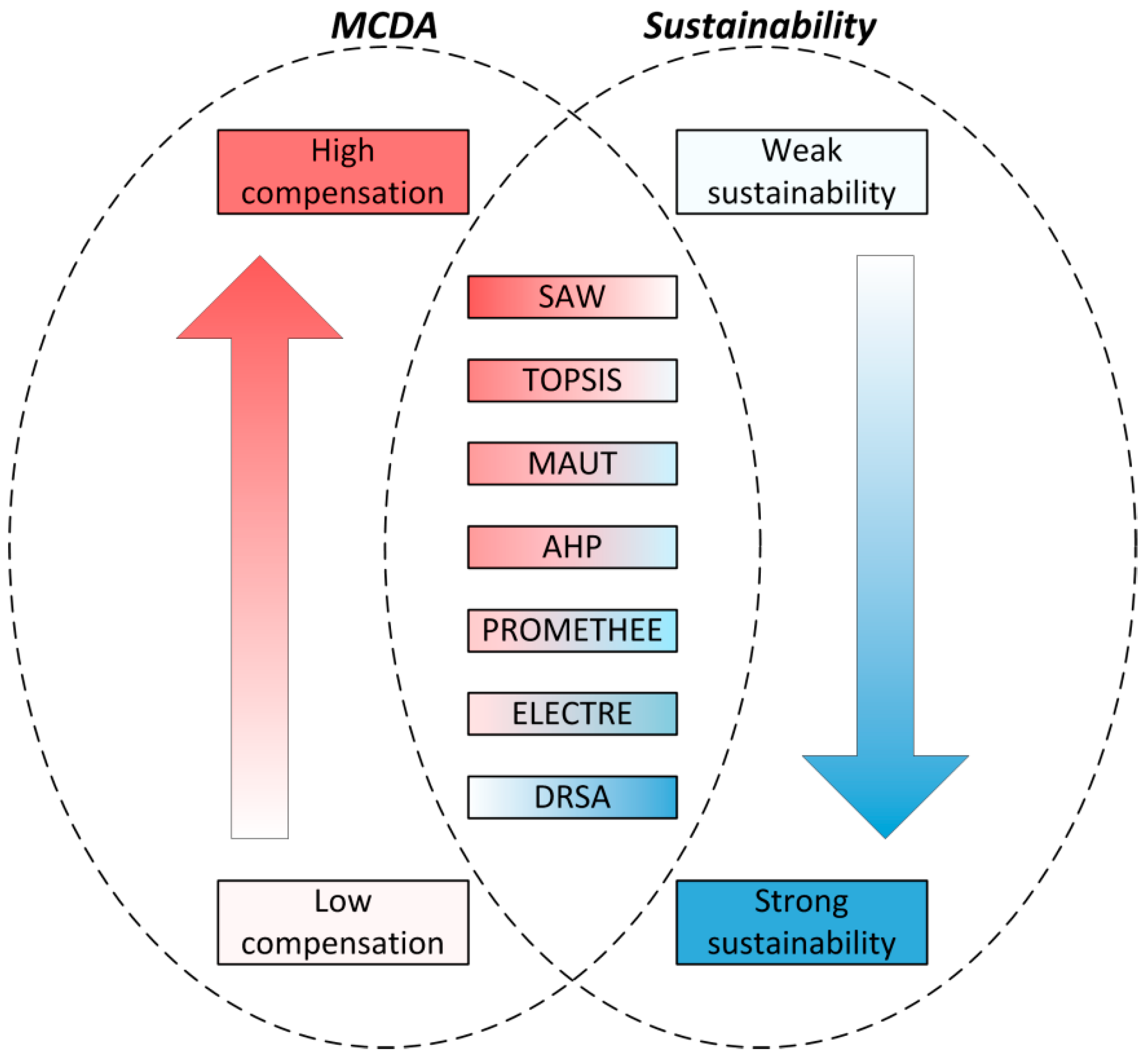
In the literature, a strong relationship between the compensation degree and weak and strong sustainability paradigms is stressed. Compensation validates substitution; therefore, compensatory methods are employed in problems related to weak sustainability, whereas non-compensatory methods are suitable for solving decision problems referring to strong sustainability [16,19]. In other words, a low compensation degree is reflected by the strong sustainability paradigm, whereas a high compensation degree corresponds to the weak sustainability paradigm.

Nevertheless, it should be noted that in many MCDA methods, the compensation degree, as well as the sustainability strength, depends on decision problem parameters provided by the decision maker. For instance, in the PROMETHEE and ELECTRE methods, the compensation degree can be adjusted to a certain extent by proper manipulation of the threshold values of indifference (q) and preference (p) [16,20]. Additionally, in the ELECTRE methods, compensation can be limited by proper values of veto thresholds (v) for criteria [16,26]. On the other hand, in the DRSA method [34], which is considered as non-compensatory [16,35], compensation is adjusted by attributes of objects/actions defined by the decision maker in a data table. For example, if in a data table consisting of two conditional attributes (criteria) c₁, c₂ and a decision attribute d, there will be an object a which has the values c₁(a) = 0, c₂(a) = 1, d(a) = 1; this means that strong compensation of a criterion c₁ by a criterion c₂ is permissible. As one can notice, in the aforementioned MCDA methods, the adjustment of a compensation degree is carried out indirectly; therefore, decision makers may find it difficult to select a proper degree of criteria compensation depending on needs, and to modify the compensation degree in order to analyse the solution to a decision problem.

Taking into consideration the difficulties with determining the compensation degree of some MCDA methods, and taking into account the fact that in many MCDA methods, the compensation degree can be adjusted, it is rational to talk about higher- or lower-degree compensation methods rather than categorizing methods such as compensatory, partially-compensatory or non-compensatory. Figure 1 presents an order of selected MCDA methods depending on their average compensation degree and a corresponding sustainability strength obtained for the decision problem solution [16,20,27,35,36,37].

2.2. PROMETHEE II and PROSA Methods

In the PROMETHEE II method, as in other MCDA methods, one can distinguish three main stages: preference modelling, aggregation and exploitation [38] (p. 163), which are elements of a five-stage decision-aid process [39]. As Bouyssou [38] (p. 165) points out, individual stages can be merged, which simplifies the PROMETHEE II computational procedure to a particular case of an additive value function model. What is more, it should be noted that the three-stage PROMETHEE II computational procedure can be conducted in two ways producing the same results [40] (p. 162): a classical one based on the aggregation of fuzzy preference relations into global preferences (aggregated preference indices) [38] (p. 163), employing net flows of a single criterion [40] (p. 197) [24] (p. 200).

The classical approach makes it possible to obtain a partial order and total order of alternatives, and can be employed in the PROMETHEE I and II methods. The approach based on single criterion net flows can be used in the PROMETHEE II method, and it can serve as the basis for GAIA analyses. Also, it can be used in the generalized PROSA method. Therefore, this approach will be presented below.

Preference modelling consists in selecting a preference function $F_j \mathrm{where} j=1\dots n$ for every criterion from among n criteria. Next, for every criterion, a fuzzy preference relation $P_j$ according to the formula (1) is calculated:

$$P_j\left(a,b\right)=F_j\left[c_j\left(a\right)-c_j\left(b\right)\right] \forall a,b\in A$$

(1)

where A is a fine set of m decision alternatives, $c_j\left(a\right)$ denotes evaluation/performance of an alternative a with regard to a criterion $c_j$.

At the aggregation stage, for every alternative a single criterion net flow with the use of the formula (2) is determined:

$${\varphi }_j\left(a\right)=\frac{1}{m-1}{\displaystyle \sum }_{b\in A}\left[P_j\left(a,b\right)-P_j\left(b,a\right)\right]$$

(2)

The last exploitation stage consists in calculating a net outranking flow according to the formula (3):

$${\varphi }_{net}\left(a\right)={\displaystyle \sum }_{j=1}^n{\varphi }_j\left(a\right) w_j$$

(3)

where $w_j$ is the weight of a criterion j, and the sum of weights is 1. The normalization of weights to 1 is carried out before the exploitation stage according to the formula (4):

$$w_j=\frac{w_j}{{\sum }_{j=1}^n w_j}$$

(4)

The ranking of alternatives is constructed on the basis of the obtained net outranking flow values.

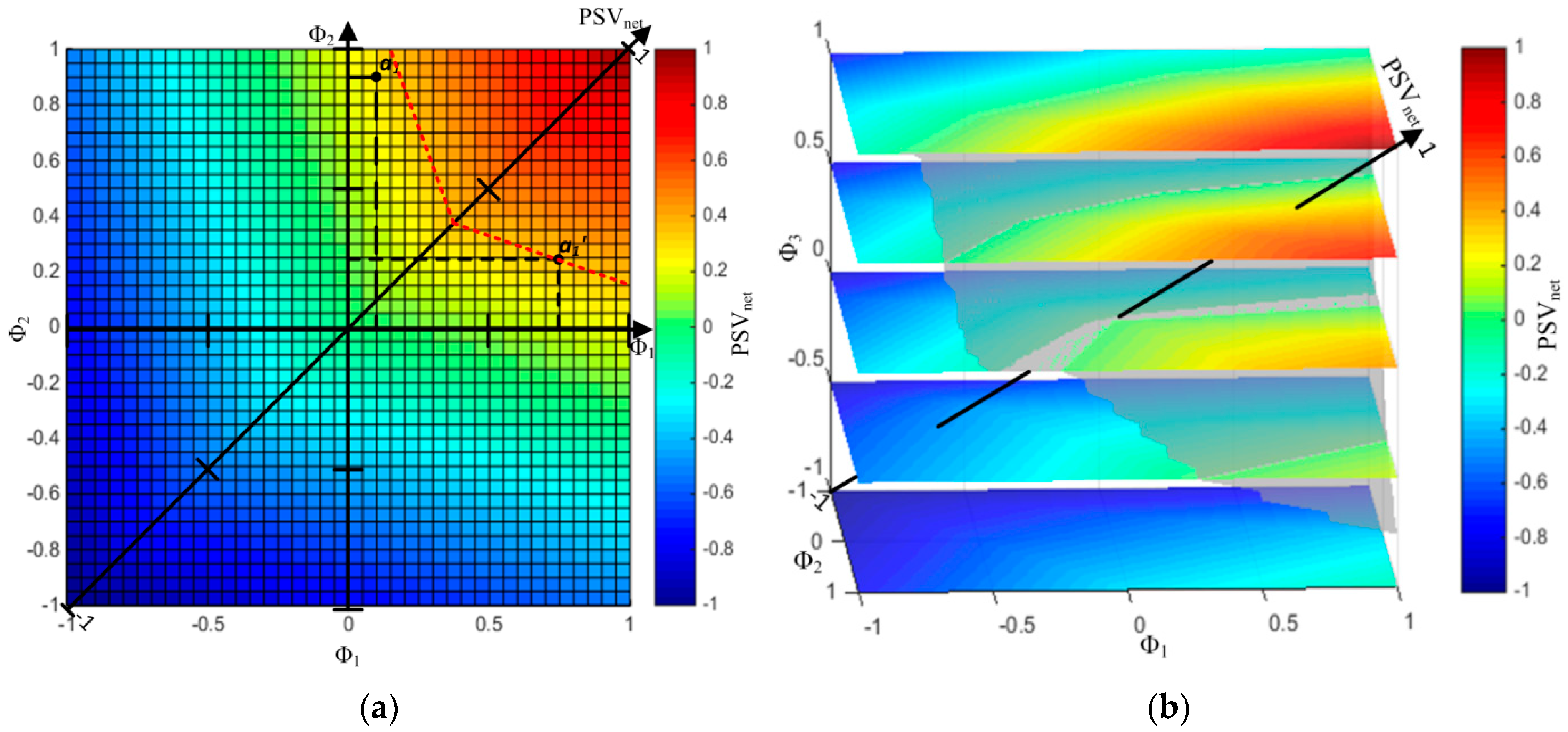
The analysis of formulas (1)–(3) allows us to notice that in the PROMETHEE II method, one can adjust the compensation degree only at the stage of preference modelling and the weights used in the method are employed as trade-offs because of the application of an additive aggregation model. This is confirmed by Figure 2, presenting a space of solutions ${\varphi }_{net}\left(a\right)$, depending on single criterion net flows obtained for two (Figure 2a) and three (Figure 2b) criteria with equal weights. Figure 2a depicts a hypothetical alternative $a_1$, whose net flow value equals ${\varphi }_1\left(a_1\right)=0.1$ and ${\varphi }_2\left(a_1\right)=0.9$. Therefore, the value ${\varphi }_{net}\left(a_1\right)=0.5$. The same value ${\varphi }_{net}$ will be assigned to an alternative $a_1^{\prime }$ where ${\varphi }_1\left(a_1^{\prime }\right)=0.75$ and ${\varphi }_2\left(a_1^{\prime }\right)=0.25$. As shown, the alternative $a_1^{\prime }$ is more sustainable than $a_1$ (low performance of a criterion $c_2\left(a_1^{\prime }\right)$ is to a lesser extent compensated by high performance of a criterion $c_1\left(a_1^{\prime }\right)$); however, according to the PROMETHEE II computational procedure, both alternatives, regardless of the sustainability of each of them, are characterized by the same performance. Generally speaking, it can be noted that for bicriteria problems, the value ${\varphi }_{net}$ is determined by a straight line orthogonal to a vector ${\varphi }_{net}$, whereas for tricriteria problems, the value ${\varphi }_{net}$ is determined by a plane orthogonal to the vector ${\varphi }_{net}$. For decision problems with a higher number of criteria, the value ${\varphi }_{net}$ is determined by analogous hyperplanes. In Figure 2b, a plane was marked which determines the location of possible alternatives for which the value ${\varphi }_{net}$ is 0, in the space of three criteria (three single criterion net flows). On the basis of Figure 2, it can be concluded that a decision alternative is sustainable if it is located in an n-dimensional space ${ℝ}^n$ near the vector ${\varphi }_{net}$, therefore it takes similar values ${\varphi }_j$ for every criterion.

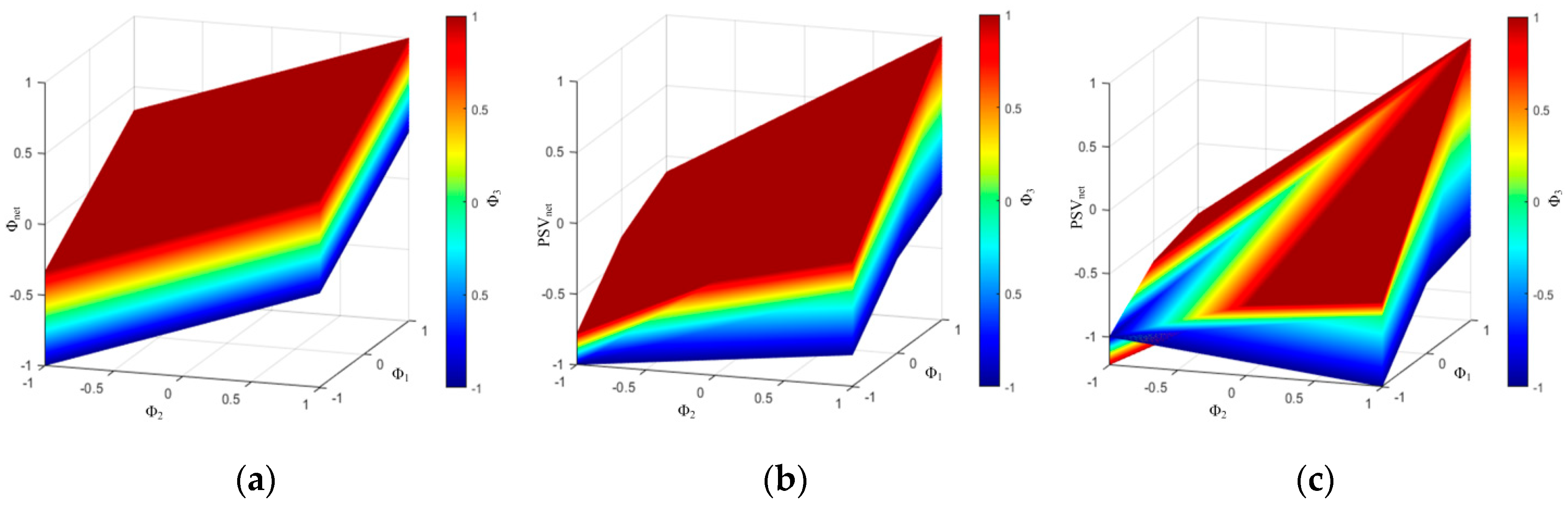
Figure 2a,b clearly depict that the value ${\varphi }_{net}$ increases linearly depending on the value of single criterion net flows and the PROMETHEE II method, when determining a ranking, does not take into consideration sustainability of alternatives. Therefore, the compensation degree of criteria, with the exception of the preference modelling stage, is high. The PROSA method is to decrease the compensation degree of criteria at the exploitation stage in such a way so that more sustainable alternatives were preferred. In addition, in the generalized PROSA method, the ability to flexibly adjust the compensation degree and to carry out the sensitivity analysis from the perspective of the compensation degree (sustainability strength) is essential.

The first version of the PROSA method [25] is an extension of the PROMETHEE II, based on four net outranking flow values. These values are calculated individually for the global result (${\varphi }_{net}$), as well as economic (${\varphi }_{net}^{Ec}$), social (${\varphi }_{net}^{So}$) and environmental (${\varphi }_{net}^{En}$) criteria. The PROSA method uses a weighted mean absolute deviation that addresses the aforementioned groups of criteria in accordance with the formula (5):

$$MA{D}_w\left(a\right)=\frac{\left|{\Phi }_{net}\left(a\right)-{\Phi }_{net}^{Ec}\left(a\right)\right|\ast w_{Ec}+\left|{\Phi }_{net}\left(a\right)-{\Phi }_{net}^{So}\left(a\right)\right|\ast w_{So}+\left|{\Phi }_{net}\left(a\right)-{\Phi }_{net}^{En}\left(a\right)\right|\ast w_{En}}{w_{Ec}+w_{So}+w_{En}}$$

(5)

As a result of the weighted MAD measure, the global assessment of alternatives in the PROSA method is based on the formula (6):

$$Value\left(a\right)={\Phi }_{net}\left(a\right)-MA{D}_w\left(a\right)$$

(6)

2.3. Justification and Research Gap

The wide usability of MCDA methods in decision problems related to sustainability is due to the fact that SD and SA problems are complex and require that many, often contradictory, criteria and uncertainties need to be considered [13,28]. The MCDA methods are designed to solve decision problems which have the characteristics (high complexity of a problem, conflicts between criteria, uncertainty), which allows their users to make decisions in a structured, transparent and reliable manner [12,16]. Moreover, the characteristics of the MCDA methods are consistent with weak and strong sustainability paradigms because of a different compensation degree of the criteria which are used in the individual methods.

An analysis of the literature indicates that in decision problems related to sustainability the following methods are most often used: WAM/SAW (Weighted Arithmetic Mean/Simple Additive Weighting), AHP, TOPSIS (Technique for Order of Preference by Similarity to Ideal Solution) and MAUT/MAVT (Multi-Attribute Utility Theory/Multi-Attribute Value Theory) [9,12,17,41]. Moreover, the majority of formal sustainability indices use a weighted average or a sum of sustainability indicators [19,21]. The following methods, characterized by a lower compensation degree, are considerably less frequently used in such decision problems: ELECTRE, PROMETHEE and DRSA (Dominance-based Rough Sets Approach) [4,12]. Therefore, decision problems in the field of sustainability are most often solved from the perspective of weak sustainability. However, as it has been noted, in decision problems of this type, the strong sustainability perspective is usually recommended [18,19,20]. Furthermore, strong sustainability is preferred in most decision contexts [35]. What is more, there is no MCDA method which would allow the decision maker to easily carry out a sensitivity analysis taking into account changes in the compensation degree and thereby changes in the sustainability strength.

From among the MCDA methods used in the context of sustainability, the PROMETHEE II method is worthy of particular attention. This method (including fuzzy versions) is widely used in decision-making problems related to sustainable development [42,43] and digital sustainability [44], and some of its unique features are useful for sustainability assessment. Thanks its use of six different preference functions, PROMETHEE II makes it possible to solve a decision problem taking into account both weaker sustainability and stronger one (higher and lower compensation degrees). This results from the fact that by fulfilling certain conditions by a preference model, and by applying the first (usual criterion) or the third (V-shape) preference function, the PROMETHEE II method works as the Borda’s method or SAW [45,46], ([38] p. 196) respectively. Both methods are characterized by a high compensation degree and also weaker sustainability [30]. On the other hand, if, for instance, the fifth preference function (V-shape with indifference area) with appropriate threshold values q and p is used, then a lower compensation degree and consequently stronger sustainability is obtained. It should be noted that the use of the thresholds q and p in PROMETHEE II makes it possible to take into account the decision maker’s uncertainty in a decision problem [47]. Furthermore, PROMETHEE enables its users to conduct a sensitivity analysis with regard to changes of weights of criteria and changes of input data which, as a result, makes it possible to analyse the reliability and robustness of a solution. Such analyses are highly recommended when solving decision problems concerning sustainability [12,17,29,48]. Moreover, PROMETHEE renders the GAIA tool accessible, which allows potential users to analyse a decision problem from a descriptive perspective. The PROMETHEE II method normalizes criteria to the scale [0, 1] and offers full comparability of alternatives with the use of the global scale [−1, 1]. Taking the process of normalization of partial evaluation into account is crucial in the PROMETHEE II method, since it is one of significant SA stages [12,17,48]. On the other hand, the ability of full comparability of alternatives is in conformity with the tendency, which has recently been visible, of using the MCDA methods, which construct a complete ranking of alternatives, in SA [12].

In [25], we presented the PROSA method based on PROMETHEE II. PROSA is characterized by a lower compensation degree than PROMETHEE II, and therefore, has stronger sustainability. This method makes it possible to use the six different preference functions used in PROMETHEE; therefore, PROSA makes it possible to modify a compensation degree and take preference uncertainty into consideration. PROSA, like PROMETHEE II, applies criteria normalization to the scale [0, 1] and allows the user to obtain a complete ranking of alternatives. Analogously to PROMETHEE, it enables its users to carry out a sensitivity analysis of a solution to changes of weights of criteria and changes of evaluations of alternatives. It should be noted that PROSA extends the PROMETHEE II computational procedure and, unlike PROMETHEE, is characterized by nonlinear sensitivity to changes of weights of criteria [25]. Moreover, PROSA, as is the case with ELECTRE III with a veto threshold, triggers ranging of alternatives with ‘well-balanced’ evaluations before ‘poorly-balanced’ alternatives [26].

Nevertheless, PROSA has also certain disadvantages. First of all, a ranking of variants is constructed only on the basis of three sustainability pillars, i.e., economic, social and environmental, without considering other sustainability dimensions. Furthermore, in the further stages of the computational procedure, it operates on sustainability dimensions without the ability to take detailed criteria into account. However, as Munda points out [30,31], in sustainability problems, using individual criteria and considering groups of criteria (dimensions) may yield different results. Also, the GAIA procedure, which would describe a decision problem from the perspective of a solution obtained via the PROSA method, has not been presented (a GAIA plane presented in [25] refers to a solution obtained with the use of the PROMETHEE method, not PROSA). Finally, PROSA, as well as PROMETHEE II and other MCDA methods, allow the user to manipulate the compensation degree only indirectly, in particular by the selection of proper preference function and by modifying the values of the thresholds q and p in the preference model. As a result, conducting a sensitivity analysis of a solution on the change of a compensation degree/sustainability strength is difficult.

Due to the aforementioned disadvantages, it is justified to undertake efforts to create a new generalized PROSA method which would derive the positive characteristics of the PROMETHEE II and PROSA methods, while at the same time avoiding their shortcomings in the context of sustainability assessment.

• The generalized PROSA ought to make it possible to consider sustainability of any dimensions and to provide the decision maker with the possibility of deciding whether SA is to be determined on the level of individual criteria or sustainability dimensions (groups of criteria).
• In addition, one needs to complete the PROSA method with the GAIA analysis which will graphically describe a solution obtained with the use of PROSA.
• A presented generalization should also provide decision makers with the ability to elastically adjust the compensation degree of individual criteria or sustainability dimensions related to sustainability of a solution.
• The adjustment of the compensation degree by decision makers ought to be conducted directly with the use of an unambiguous number coefficient in the range from the weakest to strongest sustainability.
• Moreover, the decision maker should have the ability to carry out a sensitivity analysis because of the change of the compensation degree/sustainability strength.

All requirements related to the compensation degree are inspired by Giarlotta’s postulate [49], i.e., that the compensation degree is not a characteristic of the MCDA method, but an internal/intrinsic characteristic feature of the decision maker. As a result, the generalized PROSA method should give the decision maker a broad spectrum of possibilities in terms of defining and analysing a sustainability decision problem, providing him or her with indispensable information which is necessary to verify an obtained solution both from a prescriptive perspective and a descriptive one. As indicated above, because of certain specific characteristics and their conformity with requirements of problems concerning sustainability, the PROMETHEE II method is interesting.

3. Generalized PROSA Method

The first stages of the PROSA method are analogous to PROMETHEE II, in accordance with the formulae (1)–(4). Further steps are the development of the PROMETHEE II method. Thanks to these steps, weights will be interpreted as importance coefficients and not trade-offs between criteria. Owing to the fact that the construction of a ranking on the basis of criteria may produce different results than the construction of a ranking on the basis of a group of criteria [30,31], the generalized PROSA comprises two variants of the method which conduct operations on criteria (PROSA-C) or groups of criteria (PROSA-G).

3.1. PROSA Examining Sustainability at the Criteria Level (PROSA-C)

Having determined the values ${\varphi }_{net}\left(a\right) \mathrm{and} {\varphi }_j\left(a\right)$ for j = 1, …, n, the decision maker can establish the occurrence of the sustainability/compensation relation (≈Cd, Cs) of criteria of individual decision alternatives:

• ${\varphi }_j\left(a\right)<<{\varphi }_{net}\left(a\right)$ denotes that for an alternative a, the performance of a criterion j is compensated by other criterion/criteria ($\exists {\varphi }_{j^{\prime }}\left(a\right):{\varphi }_j\left(a\right) Cd {\varphi }_{j^{\prime }}\left(a\right)$) (the alternative a is not sustainable with regard to the criterion j),
• ${\varphi }_j\left(a\right)\gg {\varphi }_{net}\left(a\right)$ denotes that for an alternative a, the performance of a criterion j compensates other criterion/criteria ($\exists {\varphi }_{j^{\prime }}\left(a\right):{\varphi }_j\left(a\right) Cs {\varphi }_{j^{\prime }}\left(a\right)$) (the alternative a is not sustainable with regard to the criterion j),
• ${\varphi }_j\left(a\right)\approx {\varphi }_{net}\left(a\right)$ denotes that an alternative a is sustainable with regard to the criterion j.

Operators >>, << denote conventional relations “much greater than” and “much less than”. The relations express the decision maker’s subjective view on whether the value on the operator’s right-hand side is much greater/much less than the value on the left-hand side, and consequently, whether the alternative a is sustainable with regard to the criterion j or not. The analysis of the sustainability/compensation relation allows the decision-maker to make assumptions about the value of the sustainability (compensation) coefficient for the criterion j ($s_j$).

In the next step, the value of a mean absolute deviation in a weighted form, where the sustainability (compensation) coefficient was taken into consideration, was determined according to the formula (7):

$$WMAD\left(a\right)={\displaystyle \sum }_{j=1}^n\left|{\varphi }_{net}\left(a\right)-{\varphi }_j\left(a\right)\right|w_j s_j$$

(7)

where $s_j$ denotes the sustainability (compensation) coefficient for a criterion j. As it can be easily noticed WMAD(a) is a sort of a weighted mean distance of a solution ${\varphi }_{net}\left(a\right)$ from solutions ${\varphi }_j\left(a\right)$ obtained for individual criteria.

The final evaluation of alternatives, i.e., $PS{V}_{net}$ (PROSA net Sustainable Value), is calculated on the basis of the formula (8):

$$PS{V}_{net}\left(a\right)={\varphi }_{net}\left(a\right)-WMAD\left(a\right)$$

(8)

Alternative steps of the PROSA-C method can be analogously written into the steps PROMETHEE II, presented in Section 2.2 in the formulae (2) and (3). In such a case, the value of the absolute deviation is calculated individually for each criterion, according to the formula (9):

$$A{D}_j\left(a\right)=\left|{\varphi }_{net}\left(a\right)-{\varphi }_j\left(a\right)\right|s_j$$

(9)

Next, for every criterion, PSV is calculated according to the formula (10):

$$PS{V}_j\left(a\right)={\varphi }_j\left(a\right)-A{D}_j\left(a\right)$$

(10)

$PS{V}_{net}$ is calculated according to the formula (11):

$$PS{V}_{net}\left(a\right)={\displaystyle \sum }_{j=1}^{n}PS{V}_j\left(a\right) w_j$$

(11)

Formulae (9)–(11) are used in the PROSA-C GAIA analysis presented in Section 3.3.

When analysing formulae (7)–(11), it should be noted that the greater the value $s_j$, the more preferred are alternatives strongly sustainable with regard to criterion j; therefore, the compensation degree for the criterion j is smaller. Theoretically, the coefficient $s_j$ can assume values form the range $\left(-\infty ,+\infty \right)$. Nevertheless, it is recommended that the value be determined in the range [0, 0.5] (see Section 3.4).

Figure 3 depicts a space of solutions $PS{V}_{net}\left(a\right)$ depending on a single criterion net flows obtained for two (Figure 3a) and three (Figure 3b) criteria which have the same weights. The values in Figure 3 were generated for a sustainability coefficient $s_j=0.5$. When comparing Figure 3a with Figure 2a, it can be noticed that the PROSA solution, unlike the PROMETHEE solution, is not linear. In the event of a bicriteria problem, considering two alternatives $a_1 \mathrm{and} a_1^{\prime }$ having equal weights and the values ${\varphi }_1\left(a_1\right)=0.1$, ${\varphi }_2\left(a_1\right)=0.9$, ${\varphi }_{net}\left(a_1\right)=0.5$, ${\varphi }_1\left(a_1^{\prime }\right)=0.75$, ${\varphi }_2\left(a_1^{\prime }\right)=0.25$, ${\varphi }_{net}\left(a_1^{\prime }\right)=0.5$ produces a result in the form of $PS{V}_{net}\left(a_1\right)=0.3$, $PS{V}_{net}\left(a_1^{\prime }\right)=0.375$; thus, a more sustainable alternative $a_1^{\prime }$ receives a better overall evaluation. The loss of linearity in the solution affects a problem consisting of three criteria. In such a case, the determined value of the solution is not located on a plane, but on a symmetrical surface which is depicted in Figure 3b for the value of $PS{V}_{net}\left(a\right)=0$.

3.2. PROSA Examining Sustainability at the Groups of Criteria Level (PROSA-G)

In the case of the PROSA-G variant, after applying the formulae (1)–(4), it is necessary to calculate the performance of groups of criteria according to the formula (12):

$${\varphi }_g{}_k\left(a\right)=\frac{{\sum }_{j=1}^{l_k}{\varphi }_j\left(a\right) w_j}{{\sum }_{j=1}^{l_k} w_j}$$

(12)

where ${\varphi }_g{}_k\left(a\right)$ denotes the net flow of an alternative a calculated for a k-th group of criteria where there are l_k criteria in the k-th group. It can be easily noticed that in the formula (12), the normalization of criteria to 1 is once again carried out, but only with a particular focus on the criteria belonging to a given group $g_k$. In practice, the same result, as the use of the formula (12), is also produced by the use of the PROMETHEE II method on a set of criteria belonging to the group $g_k$. On the basis of the value ${\varphi }_g{}_k\left(a\right)$, one can determine the sustainability/compensation of groups of criteria:

• ${\varphi }_g{}_k\left(a\right)\ll {\varphi }_{net}\left(a\right)$ denotes that for an alternative a, the performance of the k-th group of criteria is compensated by another group/other groups ($\exists {\varphi }_g{}_{k^{\prime }}\left(a\right):{\varphi }_g{}_k\left(a\right)Cd {\varphi }_g{}_{k^{\prime }}\left(a\right)$) (the alternative a is not sustainable with regard to the k-th group),
• ${\varphi }_g{}_k\left(a\right)\gg {\varphi }_{net}\left(a\right)$ denotes that for an alternative a, the performance of the k-th group of criteria compensates another group/other groups ($\exists {\varphi }_g{}_{k^{\prime }}\left(a\right):{\varphi }_g{}_k\left(a\right)Cs {\varphi }_g{}_{k^{\prime }}\left(a\right)$) (the alternative a is not sustainable with regard to the k-th group),
• ${\varphi }_g{}_k\left(a\right)\approx {\varphi }_{net}\left(a\right)$ denotes that the alternative a is sustainable with regard to the k-th group of criteria.

The value of $WMA{D}_g\left(a\right)$ is determined on the basis of the performance of groups of criteria, according to the formula (13):

$$WMA{D}_g\left(a\right)={\displaystyle \sum }_{k=1}^o\left|{\varphi }_{net}\left(a\right)-{\varphi }_g{}_k\left(a\right)\right|w_g{}_k s_g{}_k$$

(13)

where o denotes the number of groups of criteria, $s_g{}_k$ is a sustainability (compensation) coefficient for a k-th group of criteria, and $w_g{}_k$ is a weight of the k-th group of criteria, calculated as the sum of weights of all criteria belonging to the k-th group (14):

$$w_g{}_k={\displaystyle \sum }_{j=1}^{l_k}{w}_j$$

(14)

Determining $PS{V}_g{}_{net}$ takes place in the same way as in calculations on criteria in the PROSA-C variant (15):

$$PS{V}_g{}_{net}\left(a\right)={\varphi }_{net}\left(a\right)-WMA{D}_g\left(a\right)$$

(15)

As it is the case in PROSA-C, there is an alternative manner of calculating the value of $PS{V}_{net}$, with the use of the formulae (16)–(18):

$$A{D}_g{}_k\left(a\right)=\left|{\varphi }_{net}\left(a\right)-{\varphi }_g{}_k\left(a\right)\right|s_g{}_k$$

(16)

$$PS{V}_g{}_k\left(a\right)={\varphi }_g{}_k\left(a\right)-A{D}_g{}_k\left(a\right)$$

(17)

$$PS{V}_g{}_{net}\left(a\right)={\displaystyle \sum }_{k=1}^{o}PS{V}_g{}_k\left(a\right)w_g{}_k$$

(18)

This manner is employed in the PROSA-G GAIA analysis.

3.3. Geometrical Analysis for Interactive Assistance in the Generalized PROSA Method

The GAIA analysis prepared for the generalized PROSA method is a modification of the PROMETHEE-GAIA analysis presented in [24,40,50,51]. The PROSA-C GAIA and PROSA-G GAIA analyses are based on PSV performance matrices containing undermentioned values:

• $PS{V}_j(.) for j=1\dots n$, for the ROSA-C method (see the formula (10)),
• $PS{V}_g{}_k(.) for k=1\dots o$, for the PROSA-G method (see the formula (17)).

The PROSA-C GAIA analysis will be discussed below. The only difference between the two methods is that in PROSA-G GAIA instead of an n number of criteria, an o number of groups of criteria is considered and instead of the values $PS{V}_j(.)$, $PS{V}_g{}_k(.)$ are used.

In the performance matrix, an i-th alternative is represented by a row ${\alpha }_i$, which corresponds to a point $A_i$ in a space ${ℝ}^n$ (for PROSA-C GAIA). The coordinates of the space ${ℝ}^n$ are rows ${\alpha }_i$. The performance matrix for PROSA-C GAIA was depicted in the formula (19):

$$PSV=\left(\begin{array}{cccc}PS{V}_1\left(a\right)& PS{V}_2\left(a\right)& \cdots & PS{V}_n\left(a\right)\\ PS{V}_1\left(b\right)& PS{V}_2\left(b\right)& \cdots & PS{V}_n\left(b\right)\\ ⋮& ⋮& \ddots & ⋮\\ PS{V}_1\left(m\right)& PS{V}_2\left(m\right)& \cdots & PS{V}_n\left(m\right)\end{array}\right)=\left(\begin{array}{c}{\alpha }_1\\ {\alpha }_2\\ ⋮\\ {\alpha }_m\end{array}\right)$$

(19)

In order to project the space ${ℝ}^n$ on a space ${ℝ}^2$, a variance-covariance matrix is calculated (20):

$$tC=PS{V}^T·PSV$$

(20)

where C is a variance-covariance matrix, $PS{V}^T$ is the transposed matrix of $PSV$ and t is a positive integer.

On the basis of the matrix C, a set of eigenvalues $\lambda =\left\{{\lambda }_1,\dots ,{\lambda }_n\right\}$ is determined. Two biggest values from the set correspond to eigenvectors u, v (column vectors). These vectors constitute the plane ${ℝ}^2$. The number of pieces of information transferred from the plane ${ℝ}^n$ on the plane ${ℝ}^2$ can be calculated according to the formula (21):

$$\delta =\frac{{\lambda }_u+{\lambda }_v}{{\sum }_{j=1}^n{\lambda }_j}$$

(21)

The coordinates ($u_i,v_i$) of a point $A_i$ representing an i-th decision alternative on a plane are determined according to the formula (22):

$$\{\begin{array}{l}{u}_i={\alpha }_i\cdot u\\ v_i={\alpha }_i\cdot v\end{array}$$

(22)

where ${\alpha }_i$ denotes an i-th row of the matrix PSV.

The coordinates ($u_j^c,v_j^c$) of a vector representing a j-th criterion are determined according to the formula (23):

$$\{\begin{array}{l}{u}_j^c=e_j\cdot u\\ v_j^c=e_j\cdot v\end{array}$$

(23)

where $e_j$ is both a unit vector and a j-th row of an identity matrix with the size of $n\times n$.

The coordinates ($u^{\mathsf{\Pi }},v^{\mathsf{\Pi }}$) of a vector $\mathsf{\Pi }$ presenting a compromise solution are determined according to the formula (24):

$$\{\begin{array}{l}{u}^{\mathsf{\Pi }}=W\cdot u\\ v^{\mathsf{\Pi }}=W\cdot v\end{array}$$

(24)

where $W$ is a vector of normalized weights of criteria (see the formula (4)).

The interpretation of the planes PROSA-C GAIA and PROSA-G GAIA is analogous to the interpretation of the plane PROMETHEE GAIA presented, among other sources, in [52,53].

3.4. Compensation Degree and Sustainability Strength in the Generalized PROSA Method

As indicated in Section 3.1, the sustainability/compensation coefficient $s_j$ can theoretically assume values from the range of $\left(-\infty ,+\infty \right)$. If a value $s_j=0 {\forall }_{j=\left[1\dots n\right]}$, then $PS{V}_{net}(.)={\varphi }_{net}(.)$, then the solution obtained with the use of the generalized PROSA method is identical to the solution obtained with the use of the PROMETHEE II method. If the value $s_j>0$, then stronger sustainable alternatives are preferred and the compensation degree for a j-th criterion decreases. On the other hand, if the value $s_j<0$, then non-sustainable alternatives are preferred. Moreover, when analysing the formulae (7) and (8), it can be easily noticed that attributing a value from the range $[0,+\infty )$ to the coefficient $s_j$, guarantees retaining the scale $(-\infty ,1]$ for the solution $PS{V}_{net}\left(a\right)$, whereas attributing a value from the range $(-\infty ,0]$ to the coefficient $s_{j,}$ guarantees retaining the scale $[-1,+\infty )$ for the solution $PS{V}_{net}\left(a\right)$.

One of the assumptions of the generalized PROSA method was to retain, by the solution $PS{V}_{net}\left(a\right)$, a scale close to [−1, 1] applied for the solution ${\varphi }_{net}\left(a\right)$ in the PROMETHEE II method. To determine the values $s_j$ for which the scale is retained, a MATLAB simulation was carried out. For hypothetical decision problems dealing with n criteria, the value $s_j$ in the range [0.1, 1] was changed and the minimum value of $PS{V}_{net}\left(a\right)$ obtained for individual values $s_j$ and weights $w_j$ was verified. The experiment demonstrated that the influence on the obtained value of $PS{V}_{net}\left(a\right)$ equals both the value $s_j$ and the weights of criteria. For instance, for a bicriteria problem, with equal weights of both criteria, retaining the scale for the scale [−1, 1] for $PS{V}_{net}\left(a\right) \mathrm{takes} \mathrm{place}$ for the values $s_1\le 1$ and $s_2\le 1$. Nonetheless, if for the values $s_1=1$ and $s_2=1, w_1\ne w_2$ takes place, then the minimum value of $PS{V}_{net}\left(a\right)<-1$. Therefore, the experiment was conducted separately for equal weights of criteria and random weights from the range [1, 10] for every criterion. Partial results of the experiment, for equal weights of criteria and the value of the coefficient $s_j$, from the range [0.1, 1], equal for every criterion, are depicted in

Table 1. The minimum value of $PS{V}_{net}\left(a\right)$ depending on the number of criteria and the value of the coefficient s_j.

The Number of Criteria	$\mathbf{The} \mathbf{Minimum} \mathbf{Value} \mathbf{of} \mathit{P}\mathit{S}{\mathit{V}}_{\mathit{n}\mathit{e}\mathit{t}}\left(\mathit{a}\right)$
	sj = 0.1	sj = 0.2	sj = 0.3	sj = 0.4	sj = 0.5	sj = 0.6	sj = 0.7	sj = 0.8	sj = 0.9	sj = 1
n = 2	−1	−1	−1	−1	−1	−1	−1	−1	−1	−1
n = 3	−1	−1	−1	−1	−1	−1	−1	−1.0444	−1.1333	−1.2222
n = 4	−1	−1	−1	−1	−1	−1	−1.025	−1.1	−1.1750	−1.25
n = 5	−1	−1	−1	−1	−1	−1	−1.048	−1.112	−1.176	−1.24
n = 6	−1	−1	−1	−1	−1	−1	−1.0556	−1.1111	−1.1667	−1.2222
n = 7	−1	−1	−1	−1	−1	−1.0082	−1.0571	−1.1061	−1.1633	−1.2449
n = 8	−1	−1	−1	−1	−1	−1.0125	−1.0562	−1.1	−1.175	−1.25
n = 16	−1	−1	−1	−1	−1	−1.0156	−1.0562	−1.1125	−1.175	−1.25
n = 24	−1	−1	−1	−1	−1	−1.0167	−1.0563	−1.1111	−1.1771	−1.25
n = 32	−1	−1	−1	−1	−1	−1.0164	−1.0566	−1.1125	−1.1777	−1.25
n = 187	−1	−1	−1	−1	−1	−1.0167	−1.0571	−1.1125	−1.1778	−1.25

. In the experiment, it was determined that the scale [−1, 1] for the solution $PS{V}_{net}\left(a\right)$ is retained, if $s_j\le 0.5$ for equal weights of criteria. The conclusion was confirmed for a maximum of 1024 criteria. Moreover, it was found that for problems comprising 187 and more criteria, the minimum value of $PS{V}_{net}\left(a\right)$ stabilizes on constant values, as presented in Table 1.

Table 2. The minimum value of $PS{V}_{net}\left(a\right)$ obtained for 1000 draws of weights of criteria depending on the number of criteria and the value of the coefficient s_j.

The Number of Criteria	$\mathbf{The} \mathbf{Minimum} \mathbf{Value} \mathbf{of} \mathit{P}\mathit{S}{\mathit{V}}_{\mathit{n}\mathit{e}\mathit{t}}\left(\mathit{a}\right)$
	sj = 0.1	sj = 0.2	sj = 0.3	sj = 0.4	sj = 0.5	sj = 0.6	sj = 0.7	sj = 0.8	sj = 0.9	sj = 1
n = 2	−1	−1	−1	−1	−1	−1.01653	−1.05714	−1.1124	−1.17778	−1.25
n = 3	−1	−1	−1	−1	−1.0102	−1.08438	−1.16713	−1.26	−1.35578	−1.45351
n = 4	−1	−1	−1	−1	−1.0293	−1.1037	−1.18585	−1.2704	−1.36049	−1.45455
n = 5	−1	−1	−1	−1	−1.04127	−1.10926	−1.18571	−1.27041	−1.36049	−1.45455
n = 6	−1	−1	−1	−1	−1.04516	−1.10934	−1.18505	−1.26944	−1.3592	−1.45
n = 7	−1	−1	−1	−1	−1.04601	−1.10939	−1.18585	−1.26612	−1.36	−1.45238
n = 8	−1	−1	−1	−1	−1.046	−1.10934	−1.18448	−1.26479	−1.35652	−1.45238
n = 9	−1	−1	−1	−1.00117	−1.04595	−1.10809	−1.18584	−1.2656	−1.35841	−1.44726
n = 10	−1	−1	−1	−1.00209	−1.04595	−1.1077	−1.18438	−1.27013	−1.35792	−1.44987
n = 11	−1	−1	−1	−1.00293	−1.04602	−1.10934	−1.18125	−1.27025	−1.35208	−1.45222
n = 12	−1	−1	−1	−1.00384	−1.046	−1.10809	−1.18421	−1.26692	−1.35714	−1.45117
n = 13	−1	−1	−1	−1.00444	−1.04444	−1.10703	−1.18483	−1.26925	−1.35493	−1.44527
n = 14	−1	−1	−1	−1.00462	−1.04516	−1.1075	−1.18281	−1.26341	−1.35463	−1.45
n = 15	−1	−1	−1	−1.00488	−1.04545	−1.10809	−1.18257	−1.2657	−1.35284	−1.44661
n = 16	−1	−1	−1	−1.0053	−1.04525	−1.10787	−1.18395	−1.26641	−1.3536	−1.44612
n = 17	−1	−1	−1	−1.00493	−1.04561	−1.10873	−1.18262	−1.26647	−1.35496	−1.44558
n = 18	−1	−1	−1	−1.00552	−1.04602	−1.1045	−1.17879	−1.26319	−1.35817	−1.44751
n = 19	−1	−1	−1	−1.00556	−1.04575	−1.1067	−1.17782	−1.26516	−1.35425	−1.44802
n = 20	−1	−1	−1	−1.00557	−1.04602	−1.10823	−1.18285	−1.26679	−1.35333	−1.44506
n = 21	−1	−1	−1	−1.00556	−1.04528	−1.10568	−1.18284	−1.26391	−1.34965	−1.44155
n = 22	−1	−1	−1	−1.00557	−1.04524	−1.10606	−1.18465	−1.26522	−1.35499	−1.44201
n = 23	−1	−1	−1	−1.00557	−1.0441	−1.10783	−1.18024	−1.26692	−1.35299	−1.44027
n = 24	−1	−1	−1	−1.00557	−1.04402	−1.10584	−1.18073	−1.26252	−1.35033	−1.44505
n = 25	−1	−1	−1	−1.00556	−1.04334	−1.10756	−1.18044	−1.26077	−1.34733	−1.44483
n = 26	−1	−1	−1	−1.00557	−1.04492	−1.10451	−1.18036	−1.26468	−1.353	−1.44308
n = 27	−1	−1	−1	−1.00549	−1.04498	−1.10826	−1.17914	−1.26043	−1.35085	−1.44036
n = 28	−1	−1	−1	−1.00556	−1.04442	−1.10541	−1.17964	−1.26352	−1.35029	−1.44739
n = 29	−1	−1	−1	−1.00551	−1.04452	−1.1072	−1.17926	−1.26167	−1.34922	−1.44657
n = 30	−1	−1	−1	−1.00535	−1.04461	−1.107	−1.17955	−1.26525	−1.3504	−1.44161
n = 31	−1	−1	−1	−1.00538	−1.0441	−1.10517	−1.1792	−1.26281	−1.34919	−1.44571
n = 32	−1	−1	−1	−1.00539	−1.04367	−1.1049	−1.1775	−1.26311	−1.35311	−1.4432

and

Table 3. The minimum value of $PS{V}_{net}\left(a\right)$ obtained on the basis of averaging the results obtained for 1000 change events of weights of criteria depending on the number of criteria and the value of the coefficient s_j.

The Number of Criteria	$\mathbf{The} \mathbf{Minimum} \mathbf{Value} \mathbf{of} \mathit{P}\mathit{S}{\mathit{V}}_{\mathit{n}\mathit{e}\mathit{t}}\left(\mathit{a}\right)$
	sj = 0.1	sj = 0.2	sj = 0.3	sj = 0.4	sj = 0.5	sj = 0.6	sj = 0.7	sj = 0.8	sj = 0.9	sj = 1
k = 2	−1	−1	−1	−1	−1	−1.00073	−1.00744	−1.02427	−1.04241	−1.08104
k = 3	−1	−1	−1	−1	−1.00005	−1.00425	−1.02309	−1.06613	−1.13218	−1.21837
k = 4	−1	−1	−1	−1	−1.00054	−1.01323	−1.04978	−1.10773	−1.18761	−1.25969
k = 5	−1	−1	−1	−1	−1.00232	−1.02067	−1.06521	−1.13098	−1.20701	−1.28183
k = 6	−1	−1	−1	−1	−1.00354	−1.02765	−1.07656	−1.14822	−1.21905	−1.29482
k = 7	−1	−1	−1	−1	−1.00517	−1.03246	−1.08977	−1.14796	−1.22216	−1.30061
k = 8	−1	−1	−1	−1	−1.00606	−1.0367	−1.09683	−1.15795	−1.23664	−1.30953
k = 9	−1	−1	−1	−1	−1.00708	−1.04111	−1.09649	−1.16492	−1.24084	−1.32536
k = 10	−1	−1	−1	−1.00001	−1.00891	−1.04542	−1.10046	−1.1724	−1.24439	−1.32539
k = 11	−1	−1	−1	−1.00003	−1.00978	−1.04737	−1.1053	−1.17411	−1.25096	−1.3347
k = 12	−1	−1	−1	−1.00009	−1.00989	−1.04976	−1.10826	−1.17759	−1.25632	−1.34135
k = 13	−1	−1	−1	−1.00012	−1.0112	−1.05095	−1.1122	−1.18514	−1.26115	−1.3454
k = 14	−1	−1	−1	−1.00012	−1.01277	−1.05352	−1.11568	−1.1871	−1.26605	−1.34704
k = 15	−1	−1	−1	−1.00015	−1.01314	−1.05458	−1.11536	−1.19187	−1.26889	−1.35159
k = 16	−1	−1	−1	−1.00018	−1.01372	−1.05696	−1.12081	−1.19037	−1.27058	−1.35438
k = 17	−1	−1	−1	−1.00017	−1.01423	−1.05928	−1.12124	−1.19253	−1.27177	−1.3581
k = 18	−1	−1	−1	−1.00021	−1.01537	−1.05965	−1.12318	−1.19824	−1.27802	−1.35596
k = 19	−1	−1	−1	−1.00024	−1.0152	−1.06068	−1.12452	−1.19753	−1.27741	−1.36291
k = 20	−1	−1	−1	−1.00029	−1.01673	−1.06207	−1.12829	−1.1993	−1.28053	−1.36674
k = 21	−1	−1	−1	−1.00027	−1.01614	−1.06227	−1.12933	−1.20334	−1.28156	−1.36758
k = 22	−1	−1	−1	−1.00028	−1.01767	−1.06509	−1.13001	−1.20528	−1.28362	−1.37185
k = 23	−1	−1	−1	−1.00032	−1.01832	−1.06677	−1.13017	−1.20461	−1.28523	−1.36906
k = 24	−1	−1	−1	−1.00028	−1.01786	−1.06719	−1.12994	−1.20625	−1.28757	−1.37285
k = 25	−1	−1	−1	−1.00035	−1.01894	−1.06701	−1.13239	−1.20934	−1.288	−1.37466
k = 26	−1	−1	−1	−1.0003	−1.0192	−1.06804	−1.13409	−1.20783	−1.29214	−1.37931
k = 27	−1	−1	−1	−1.00042	−1.02071	−1.06855	−1.13452	−1.21069	−1.29173	−1.37717
k = 28	−1	−1	−1	−1.00038	−1.02023	−1.069	−1.13689	−1.21158	−1.29383	−1.38108
k = 29	−1	−1	−1	−1.00038	−1.02039	−1.07038	−1.13547	−1.21483	−1.29314	−1.37922
k = 30	−1	−1	−1	−1.00037	−1.02098	−1.07108	−1.13768	−1.21533	−1.29732	−1.38276
k = 31	−1	−1	−1	−1.00048	−1.0216	−1.07243	−1.13813	−1.21439	−1.29952	−1.38308
k = 32	−1	−1	−1	−1.00042	−1.02067	−1.07162	−1.13905	−1.21733	−1.29846	−1.38409

present respectively the minimum and average (for 1000 draws) values of $PS{V}_{net}\left(a\right)$ obtained for various and random weights of criteria (for decision problems from 2 up to 32 criteria).

On the basis on the results depicted in Table 2 and Table 3, it should be noted that if the decision maker insists on retaining the scale [−1, 1] for final solutions, then the values of $s_j$ ought not to be greater than 0.3, on the assumption that the weights of criteria are different. In practice, attributing the value 0.5 by the coefficient $s_j$ is permissible, since the minimum value of $PS{V}_{net}\left(a\right)$ only slightly exceeds −1. However, assuming equal weights of criteria to retain the scale [−1, 1] for $PS{V}_{net}\left(a\right)$, one needs to set the values of $s_j$ in the range [0, 0.5]. Nevertheless, if the decision maker wants to reward sustainable alternatives, and retaining the scale [−1, 1] is not essential for him or her, then the value of the sustainability coefficient $s_j$ may exceed the values of 0.3 or 0.5. Figure 4 shows a comparison of a space of solutions ${\varphi }_{net}$ (Figure 4a) and $PS{V}_{net}$ with the use of the sustainability/compensation coefficient $s_j=0.5$ (Figure 4b) and $s_j=1$ (Figure 4c) for three criteria with equal weights.

The analysis of Figure 4 indicates that in the case of the solutions $PS{V}_{net}$, where $s_j=0.5$, then single criterion net flows have a more significant influence on overall performance (the value of $PS{V}_{net}$) than the sustainability/compensation coefficient $s_j$. On the other hand, when $s_j=1$, then this coefficient has a more significant influence on the solution than the values of single criterion net flows. As a result, the strongest sustainable alternatives are preferred. The confirmation of this observation is the fact that in the case of $s_j=1$, the value of $PS{V}_{net}$ is greater for ${\varphi }_1={\varphi }_2={\varphi }_3$ than for ${\varphi }_3>{\varphi }_1={\varphi }_2$. To sum up the conducted research, with the assumption of equal weights of criteria, the value $s_j\le 0.5$ makes it possible for the value $PS{V}_{net}\left(a\right)$ not to exceed the range [−1, 1], and the influence of criteria sustainability on the solution will not be greater than the influence of the value ${\varphi }_j\left(a\right).$ On the other hand, on the assumption that the weights of criteria are different, setting the value $s_j\le 0.3$ makes it possible to retain the scale [−1, 1] for $PS{V}_{net}\left(a\right)$. All the presented conclusions refer both to the PROSA-C method and the PROSA-G method.

4. Illustrative Application and Discussion

The use of PROSA-C and PROSA-G methods will be described on the basis of a decision problem presented in the article [54]. The problem was selected since it deals with sustainability, and it presents a considerably high number of sustainability dimensions. Moreover, the authors define indifference and preference thresholds for criteria.

4.1. The Use of the PROSA-C and PROSA-G Methods in a Sustainability Decision Problem

The presented decision problem concerns the selection of a sustainable demolition waste management strategy. Article defines 9 strategy alternatives which are considered with regard to 12 criteria belonging to 6 groups of criteria (sustainability dimensions). The problem in the article [54] was solved with the use of the ELECTRE III method; therefore, the authors applied indifference, preference and veto thresholds. Criteria, groups of criteria, weights, thresholds, preference directions, preference functions considered in the decision problem are shown in

Table 4. Criteria and their parameters considered in the decision problem.

Group of Criteria	Criterion	Weight	Preference Direction	Preference Function	Indifference Threshold (q)	Preference Threshold (p)
G1—Environmental	C1—Lost energy (GJ)	0.3333	Min	V-shape with indifference threshold	420	2100
	C2—Flows of abiotic materials (t)	0.1667	Min		1000	5000
	C3—Recovery ratio (%)	0.1667	Max		10	50
	C4—Global warming (t co2)	0.3333	Min		40	200
G2—Socio- Environmental	C5—Positive performances of pollutants	0.25	Max		1	5
	C6—Negative performances of pollutants	0.75	Max		7	20
G3—Economic	C7—Financial cost of demolition (k€)	1	Min		50	100
G4—Economic and Environmental	C8—Economic activity generated by recycled materials (k€)	1	Max		20	80
G5—Social	C9—Areas destroyed (ha)	0.4	Max		1	4
	C10—Duration of demolition (months)	0.20	Min		1	2
	C11—Impact of the trucks	0.40	Min		4.6	23
G6—Socio- Economic	C12—Employment	1	Max		1	3

, whereas

Table 5. Evaluations of alternatives for every criterion.

Group of Criteria	Criterion	A1	A2	A3	A4	A5	A6	A7	A8	A9
G1	C1	38723	34913	25596	34842	22570	39773	19500	34525	16486
	C2	33207	32085	2123	32095	1445	17485	868	16958	958
	C3	0	0.2	5	0.2	0.2	0.2	99	99	99
	C4	3375	3127	3547	3115	3090	4135	3160	4295	3653
G2	C5	11.36	12.78	12.78	12.86	12.86	17	12.86	17	12.86
	C6	−320.9	−148.4	−148.4	−9.9	−9.9	0	−9.9	0	−9.9
G3	C7	203.7	463	356.2	552.5	295	383	264	352	264
G4	C8	0	11.7	44.8	11.7	95.9	95.9	116.8	116.8	164.9
G5	C9	0	4.9	10.7	5.4	11.2	11.2	11.2	11.2	11.2
	C10	1	1	1	3.5	4	4	4	4	4
	C11	21.5	47.9	27.7	39.7	1.5	22.7	2.7	23.9	1
G6	C12	0	3.7	4.5	10.3	11.5	11.5	11.3	11.3	11.4

presents evaluations of alternatives for every criterion.

As a result of applying the PROMETHEE II method, the values ${\varphi }_j \mathrm{and} {\varphi }_{net}$, presented in

Table 6. Values ${\varphi }_j \mathrm{and} {\varphi }_{net}$ obtained with the use of the PROMETHEE II method.

Criterion	A1	A2	A3	A4	A5	A6	A7	A8	A9
${\varphi }_1$	−0.8281	−0.25	0.25	−0.25	0.5	−0.9219	0.75	−0.25	1
${\varphi }_2$	−0.7573	−0.7462	0.6119	−0.7465	0.625	−0.125	0.633	−0.125	0.6302
${\varphi }_3$	−0.375	−0.375	−0.375	−0.375	−0.375	−0.375	0.75	0.75	0.75
${\varphi }_4$	−0.0219	0.625	−0.3016	0.6289	0.6484	−0.7813	0.5977	−0.9688	−0.4266
${\varphi }_5$	−0.3388	−0.1881	−0.1881	−0.1806	−0.1806	0.7188	−0.1806	0.7188	−0.1806
${\varphi }_6$	−1	−0.625	−0.625	0.3192	0.3192	0.4865	0.3192	0.4865	0.3192
${\varphi }_7$	0.7798	−0.7263	−0.114	−0.9738	0.2873	−0.27	0.5498	−0.0825	0.5498
${\varphi }_8$	−0.6767	−0.6523	−0.365	−0.6523	0.334	0.334	0.4285	0.4285	0.8213
${\varphi }_9$	−1	−0.625	0.375	−0.625	0.375	0.375	0.375	0.375	0.375
${\varphi }_{10}$	0.75	0.75	0.75	−0.375	−0.375	−0.375	−0.375	−0.375	−0.375
${\varphi }_{11}$	−0.0808	−0.8804	−0.2323	−0.6535	0.7133	−0.1216	0.6889	−0.1569	0.7235
${\varphi }_{12}$	−1	−0.625	−0.625	0.3438	0.3875	0.3875	0.375	0.375	0.3813
${\varphi }_{net}$	−0.4143	−0.5056	−0.2317	−0.2892	0.3313	0.0619	0.4296	0.1626	0.4553

, were obtained.

Next, PROSA-C and PROSA-G computational procedures were conducted. In the PROSA-C method, the further step was to determine the sustainability and compensation of criteria. The value ${\varphi }_{net}\left(a\right)-{\varphi }_j\left(a\right)>0.1$ was set as the limit value which makes it possible to differentiate the relations of sustainability (≈), being compensated (Cd) and compensating (Cs). These relations are shown in

Table 7. Sustainability/compensation relations between the values ${\varphi }_j$ in the PROSA-C method.

Criterion	A1	A2	A3	A4	A5	A6	A7	A8	A9	Cardinality (≈)	Cardinality (Cd)	Cardinality (Cs)
${\varphi }_1$	Cd	Cs	Cs	≈	Cs	Cd	Cs	Cd	Cs	1	3	5
${\varphi }_2$	Cd	Cd	Cs	Cd	Cs	Cd	Cs	Cd	Cs	0	5	4
${\varphi }_3$	≈	Cs	Cd	≈	Cd	Cd	Cs	Cs	Cs	2	3	4
${\varphi }_4$	Cs	Cs	≈	Cs	Cs	Cd	Cs	Cd	Cd	1	3	5
${\varphi }_5$	≈	Cs	≈	Cs	Cd	Cs	Cd	Cs	Cd	2	3	4
${\varphi }_6$	Cd	Cd	Cd	Cs	≈	Cs	Cd	Cs	Cd	1	5	3
${\varphi }_7$	Cs	Cd	Cs	Cd	≈	Cd	Cs	Cd	≈	2	4	3
${\varphi }_8$	Cd	Cd	Cd	Cd	≈	Cs	≈	Cs	Cs	2	4	3
${\varphi }_9$	Cd	Cd	Cs	Cd	≈	Cs	≈	Cs	≈	3	3	3
${\varphi }_{10}$	Cs	Cs	Cs	≈	Cd	Cd	Cd	Cd	Cd	1	5	3
${\varphi }_{11}$	Cs	Cd	≈	Cd	Cs	Cd	Cs	Cd	Cs	1	4	4
${\varphi }_{12}$	Cd	Cd	Cd	Cs	≈	Cs	≈	Cs	≈	3	3	3

.

When analysing Table 7, it should be noted that the most sustainable criteria are C9 and C12, which ensure sustainability for 3 decision alternatives. On the other hand, the least sustainable criterion is C2. Based on the analysis of Table 7, in the PROSA-C method, the values of sustainability/compensation coefficients were set as $s_j=0.5-Cardinality(\approx )\times 0.1$. The values of $s_j$ are depicted in

Table 8. The values of the coefficient $s_j$ for the criteria.

${\mathit{s}}_1$	${\mathit{s}}_2$	${\mathit{s}}_3$	${\mathit{s}}_4$	${\mathit{s}}_5$	${\mathit{s}}_6$	${\mathit{s}}_7$	${\mathit{s}}_8$	${\mathit{s}}_9$	${\mathit{s}}_{10}$	${\mathit{s}}_{11}$	${\mathit{s}}_{12}$
0.4	0.5	0.3	0.4	0.3	0.4	0.3	0.3	0.2	0.4	0.4	0.2

.

The weighted values of a mean absolute deviation for individual alternatives, their values $PS{V}_{net}$ and positions in the PROSA-C ranking are depicted in

Table 9. The values WMAD, $PS{V}_{net}$ and their positions in the PROSA-C ranking.

	A1	A2	A3	A4	A5	A6	A7	A8	A9
WMAD	0.1778	0.0959	0.0922	0.1489	0.0522	0.1322	0.0557	0.1175	0.0961
$PS{V}_{net}$	−0.5921	−0.6014	−0.3240	−0.4381	0.2791	−0.0703	0.3739	0.0451	0.3592
Rank	8	9	6	7	3	5	1	4	2

.

In the PROSA-G method, the values ${\varphi }_g{}_k$ for every k-th group of criteria were calculated. These values are shown in

Table 10. The values ${\varphi }_g{}_k \mathrm{and} {\varphi }_{net}$.

Group	A1	A2	A3	A4	A5	A6	A7	A8	A9
${\varphi }_g{}_1$	−0.4721	−0.0619	0.0223	−0.0606	0.4245	−0.651	0.6797	−0.3021	0.4212
${\varphi }_g{}_2$	−0.8347	−0.5158	−0.5158	0.1943	0.1943	0.5446	0.1943	0.5446	0.1943
${\varphi }_g{}_3$	0.7798	−0.7263	−0.114	−0.9738	0.2873	−0.27	0.5498	−0.0825	0.5498
${\varphi }_g{}_4$	−0.6767	−0.6523	−0.365	−0.6523	0.334	0.334	0.4285	0.4285	0.8213
${\varphi }_g{}_5$	−0.2823	−0.4522	0.2071	−0.5864	0.3603	0.0264	0.3505	0.0122	0.3644
${\varphi }_g{}_6$	−1	−0.625	−0.625	0.3438	0.3875	0.3875	0.375	0.375	0.3813
${\varphi }_{net}$	−0.4143	−0.5056	−0.2317	−0.2892	0.3313	0.0619	0.4296	0.1626	0.4553

.

As in the PROSA-C method, in PROSA-G, the limit value which makes it possible to differentiate the sustainability and compensation relations was the value ${\varphi }_{net}\left(a\right)-{\varphi }_g{}_k\left(a\right)>0.1$. These relations are presented in

Table 11. Sustainability/compensation relations between the values ${\varphi }_g{}_k$.

Group	A1	A2	A3	A4	A5	A6	A7	A8	A9	Cardinality (≈)	Cardinality (Cd)	Cardinality (Cs)
${\varphi }_g{}_1$	≈	Cs	Cs	Cs	≈	Cd	Cs	Cd	≈	3	2	4
${\varphi }_g{}_2$	Cd	≈	Cd	Cs	Cd	Cs	Cd	Cs	Cd	1	5	3
${\varphi }_g{}_3$	Cs	Cd	Cs	Cd	≈	Cd	Cs	Cd	≈	2	4	3
${\varphi }_g{}_4$	Cd	Cd	Cd	Cd	≈	Cs	≈	Cs	Cs	2	4	3
${\varphi }_g{}_5$	Cs	≈	Cs	Cd	≈	≈	≈	Cd	≈	5	2	2
${\varphi }_g{}_6$	Cd	Cd	Cd	Cs	≈	Cs	≈	Cs	≈	3	3	3

.

The analysis of Table 11 indicates that in the case of the PROSA-G method, the most sustainable group of criteria is G5. On the other hand, the least sustainable group is G2. Based on the analysis of Table 11, in the PROSA-G method, the values of sustainability/compensation coefficients for groups of criteria were set as $s_g{}_k=0.5-Cardinality(\approx )\times 0.1$. The values of $s_g{}_k$ are depicted in

Table 12. The values of the coefficient $s_g{}_k$ for the groups of criteria.

${\mathit{s}}_{\mathit{g}}{}_1$	${\mathit{s}}_{\mathit{g}}{}_2$	${\mathit{s}}_{\mathit{g}}{}_3$	${\mathit{s}}_{\mathit{g}}{}_4$	${\mathit{s}}_{\mathit{g}}{}_5$	${\mathit{s}}_{\mathit{g}}{}_6$
0.2	0.4	0.3	0.3	0	0.2

.

The weighted values of a mean absolute deviation for individual alternatives, their values $PS{V}_{net}$ and positions in the PROSA-G ranking are depicted in

Table 13. The values of $WMA{D}_g$, $PS{V}_g{}_{net}$ and positions in the PROSA-G ranking.

	A1	A2	A3	A4	A5	A6	A7	A8	A9
$WMA{D}_g$	0.1223	0.0378	0.0531	0.1133	0.0165	0.097	0.0319	0.0736	0.044
$PS{V}_g{}_{net}$	−0.5366	−0.5434	−0.2848	−0.4025	0.3148	−0.0351	0.3977	0.089	0.4113
Rank	8	9	6	7	3	5	2	4	1

.

When analysing the rankings obtained with the use of the methods PROSA-C and PROSA-G (see Table 9 and Table 13), it can be easily noticed that both variants of the generalized PROSA method produce somewhat different results. This results, first of all, from the fact that in the case of PROSA-C, the value $PS{V}_{net}$ is determined on the basis of the performance of criteria, whereas in PROSA-G, on the basis of the performance of groups of criteria. The performances are different from one another, whereas the overall performance ${\varphi }_{net}$ will be the same for the criteria and the groups. On the basis of the formula (12), it can be noted that ${\varphi }_g{}_k$ of a k-th group of criteria is a weighted arithmetic mean of the performance of all the criteria in the group. On the other hand, the overall performance ${\varphi }_{net}$ is a weighted arithmetic mean of all criteria in all the groups. Therefore, the values $WMA{D}_g$/$A{D}_g$ for the groups of the criteria in the PROSA-G method will usually be lower than the values WMAD/AD for the criteria in PROSA-C. As a consequence, in the PROSA-G method, greater values $PS{V}_{net}$ than in the PROSA-C variant will be most often be obtained. Apart from the comparison of the two variants of the generalized PROSA method, the comparison of the PROSA-C and PROSA-G rankings with the rankings obtained with the use of other MCDA methods characterized by a different compensation degree also seems to be a challenging issue.

4.2. The Comparison of the PROSA-C and PROSA-G Ranking with the Rankings of other MCDA Methods

The PROSA-C and PROSA-G rankings were compared to those obtained with the use of methods characterized by a relatively high or low compensation degree (weak and strong sustainability). From among high compensation degree methods, the following ones took part in the comparison: SAW [55], TOPSIS [55] and AHP [56]. On the other hand, low compensation degree methods were represented by WP (Weighted Product) [57], PROMETHEE I [24], PROMETHEE II [24], ELECTRE III [33] and ELECTRE Is [33]. All the methods, apart from ELECTRE Is, consider the problematic γ; therefore, they generate a ranking of alternatives, whereas ELECTRE Is deals with the problematic α generating a graph kernel of alternatives. Furthermore, the PROMETHEE I and ELECTRE III methods generate a partial order of alternatives. Thus, for the ranking obtained in the methods, a ‘median order’ was also generated [58], which is a sort of a total order. Other methods make it possible to obtain a total order of alternatives. In methods considering the veto threshold, v=46 for a criterion C5 was applied in accordance with [54]. Furthermore, for the ELECTRE Is method, a concordance level=0.8 was used. Rankings obtained with the use of individual MCDA methods and the graph kernel calculated in the ELECTRE Is method are shown in

Table 14. Rankings obtained in various MCDA methods.

MCDA Method	Rank
	1	2	3	4	5	6	7	8	9
PROSA-C	A7	A9	A5	A8	A6	A3	A4	A1	A2
PROSA-G	A9	A7	A5	A8	A6	A3	A4	A1	A2
SAW	A9	A8	A7	A6	A5	A3	A4	A2	A1
TOPSIS	A9	A7	A8	A5	A6	A4	A3	A2	A1
AHP	A8	A9	A6	A7	A5	A3	A4	A1	A2
WP	A8	A6	A9	A7	A5	A3	A4	A2	A1
PROMETHEE I (median order)	A7/A9	-	A5	A8	A6	A3	A1/A4	-	A2
PROMETHEE II	A9	A7	A5	A8	A6	A3	A4	A1	A2
ELECTRE III (median order)	A9	A7	A5	A8	A6	A1/A3	-	A4	A2
ELECTRE Is (kernel)	A5/A7/A9	-	-	-	-	-	-	-	-
PROMETHEE I (partial order)
ELECTRE III (partial order)

. The analysis of Table 14 clearly indicates that in the majority of the rankings, the first position takes an alternative A9. Moreover, in the methods based on the outranking relations, the best three alternatives are always A5, A7 and A9. The comparison of the generalized PROSA and PROMETHEE rankings is interesting. As pointed out in Section 3.4, if in the PROSA-C method, the value s=0 for every criterion, then the obtained solution is identical to PROMETHEE II. The analysis of Table 14 clearly indicates that the introduction of positive coefficients s_j for criteria made the alternatives A7 and A9 change their places in the PROSA-C and PROMETHEE II rankings. What is more, in the PROMETHEE I ranking, the alternatives A7 and A9 were considered as non-comparable (partial order) or indifferent (median order). As a result of taking into consideration the assumed values of the coefficients s_j in the PROSA-C solution, the relation between these alternatives was set in favour of A7, as opposed to the PROMETHEE II solution, in which A9 was a more preferred alternative.

Moreover, the correlation between the ranking obtained with the use of individual MCDA methods was examined. The role of variables was played by the rankings of individual methods and the positions of individual alternatives in the ranking were treated as observations. Owing to the fact that rankings have an ordinal not quantitative character, the use of nonparametric correlation coefficients, i.e., Spearman’s rho and Kendall’s tau [59], was considered. It should be noted that in the literature it is recommended to use Kendall’s tau instead of Spearman’s rho [60,61] (p. 306) [62] (chapter 7.4.4). Therefore, to examine the correlations between the rankings of various MCDA method, Kendall’s tau was used. The results of the research into the correlations between the rankings are presented in

Table 15. Kendall’s tau’s correlations between the rankings.

	PROSA-C	PROSA- G	PROMETHEE II	PROMETHEE I	ELECTRE III	SAW	TOPSIS	AHP	WP
PROSA-C	1	0.9444	0.9444	0.9718	0.8733	0.7222	0.7778	0.6667	0.5556
PROSA G	0.9444	1	1.0000	0.9718	0.9297	0.7778	0.8333	0.7222	0.6111
PROMETHEE II	0.9444	1.0000	1	0.9718	0.9297	0.7778	0.8333	0.7222	0.6111
PROMETHEE I	0.9718	0.9718	0.9718	1	0.9566	0.7432	0.8003	0.6860	0.5717
ELECTRE III	0.8733	0.9297	0.9297	0.9566	1	0.7043	0.7606	0.6480	0.5353
SAW	0.7222	0.7778	0.7778	0.7432	0.7043	1	0.8333	0.8333	0.8333
TOPSIS	0.7778	0.8333	0.8333	0.8003	0.7606	0.8333	1	0.6667	0.6667
AHP	0.6667	0.7222	0.7222	0.6860	0.6480	0.8333	0.6667	1	0.8889
WP	0.5556	0.6111	0.6111	0.5717	0.5353	0.8333	0.6667	0.8889	1

. It should be noted that for every correlation value presented in Table 15, a significance p < 0.05 was obtained.

The analysis of Table 15 indicates that in the considered decision problem, the PROSA-C method produces results which are closest to the PROMETHEE I method and PROSA-G generated a ranking identical to the PROMETHEE II ranking. Moreover, the PROSA-C and PROSA-G rankings are also similar to the ELECTRE III ranking. It results from the methodological similarity of the methods, since PROSA, just as PROMETHEE and ELECTRE, is based on the outranking relation and employs indifference and preference thresholds. On the other hand, the SAW, TOPSIS, AHP and WP methods use a single synthesizing criterion and a similarity of their rankings to the rankings obtained with the use of outranking methods is considerably lower. When analysing the correlations between the rankings obtained with the use of methods based on a single synthesizing criterion, it should be noted that the SAW ranking is strongly correlated to the TOPSIS, AHP and WP rankings. To some extent, this results from the fact that in all the methods, normalisation is applied (linear scale transformation in the case of SAW, AHP, WP and vector normalization in TOPSIS). In addition, the WP ranking is strongly correlated with the SAW and AHP rankings and weakly correlated with TOPSIS. Probably, the reason for the indicated similarities, at least partially, is the same type of normalization in the WP, SAW, AHP methods and another type of normalization in TOPSIS. The strong correlation of the WP ranking with the SAW and AHP rankings and the weak correlation with the rankings of the outranking methods indicate that the methodical similarities in individual MCDA methods more strongly influence the order of alternatives in a ranking than an estimated compensation degree of a given method. The conclusion was drawn on the basis of weighing the discussed correlation with the fact cited in Section 2.1 stating that methods applying multiplicative aggregation are less compensatory than additive aggregation methods, and outranking methods are less compensatory than methods based on a single synthesizing criterion.

4.3. Comparison of the Results of the GAIA Analysis in the PROSA and PROMETHEE Methods

In order to carry out the PROSA-C GAIA analysis, firstly, the values of AD on the basis of values ${\varphi }_{net}$, ${\varphi }_j$ (see Table 6) and $s_j$ (see Table 8) were determined. The values of $A{D}_j$ for criteria in the PROSA-C method are shown in

Table 16. The values of $A{D}_j$ determined in the PROSA-C method.

Criterion	A1	A2	A3	A4	A5	A6	A7	A8	A9
$A{D}_1$	0.4138	0.2556	0.4817	0.0392	0.1687	0.9838	0.3204	0.4126	0.5447
$A{D}_2$	0.3430	0.2406	0.8436	0.4573	0.2937	0.1869	0.2033	0.2876	0.1748
$A{D}_3$	0.0393	0.1306	0.1433	0.0858	0.7063	0.4369	0.3204	0.5874	0.2947
$A{D}_4$	0.3925	1.1306	0.0698	0.9181	0.3171	0.8431	0.1680	1.1314	0.8819
$A{D}_5$	0.0756	0.3174	0.0436	0.1086	0.5119	0.6569	0.6103	0.5561	0.6360
$A{D}_6$	0.5857	0.1194	0.3933	0.6084	0.0121	0.4246	0.1104	0.3239	0.1361
$A{D}_7$	1.1941	0.2207	0.1177	0.6846	0.0440	0.3319	0.1201	0.2451	0.0944
$A{D}_8$	0.2623	0.1467	0.1333	0.3631	0.0027	0.2721	0.0011	0.2659	0.3659
$A{D}_9$	0.5857	0.1194	0.6067	0.3358	0.0437	0.3131	0.0546	0.2124	0.0803
$A{D}_{10}$	1.1643	1.2556	0.9817	0.0858	0.7063	0.4369	0.8046	0.5376	0.8303
$A{D}_{11}$	0.3335	0.3749	0.0006	0.3644	0.3820	0.1835	0.2592	0.3196	0.2682
$A{D}_{12}$	0.5857	0.1194	0.3933	0.6329	0.0562	0.3256	0.0546	0.2124	0.0741

. On the basis of the values of $A{D}_j$, the values of $PS{V}_j$ presented in

Table 17. The values of $PS{V}_j$ determined in the PROSA-C method.

Criterion	A1	A2	A3	A4	A5	A6	A7	A8	A9
$PS{V}_1$	−0.9936	−0.3522	0.0573	−0.2657	0.4325	−1.3154	0.6219	−0.4151	0.7821
$PS{V}_2$	−0.9288	−0.8665	0.1901	−0.9752	0.4781	−0.2184	0.5313	−0.2688	0.5428
$PS{V}_3$	−0.3868	−0.4142	−0.4180	−0.4007	−0.5869	−0.5061	0.6539	0.5738	0.6616
$PS{V}_4$	−0.1789	0.1728	−0.3295	0.2617	0.5216	−1.1185	0.5304	−1.4213	−0.7793
$PS{V}_5$	−0.3614	−0.2834	−0.2012	−0.2132	−0.3342	0.5217	−0.3637	0.5519	−0.3714
$PS{V}_6$	−1.2343	−0.6728	−0.7823	0.0759	0.3144	0.3167	0.2751	0.3570	0.2648
$PS{V}_7$	0.4215	−0.7925	−0.1493	−1.1791	0.2740	−0.3696	0.5137	−0.1560	0.5214
$PS{V}_8$	−0.7554	−0.6963	−0.4050	−0.7612	0.3332	0.2523	0.4282	0.3488	0.7115
$PS{V}_9$	−1.1171	−0.6489	0.2537	−0.6922	0.3663	0.3124	0.3641	0.3325	0.3589
$PS{V}_{10}$	0.2843	0.2478	0.3573	−0.4093	−0.6575	−0.5498	−0.6969	−0.5901	−0.7071
$PS{V}_{11}$	−0.2142	−1.0304	−0.2326	−0.7993	0.5605	−0.1950	0.5852	−0.2848	0.6162
$PS{V}_{12}$	−1.1171	−0.6489	−0.7037	0.2172	0.3763	0.3224	0.3641	0.3325	0.3664

were determined. If the matrix presented in Table 17 is transposed, a performance matrix for PROSA-C GAIA will be obtained.

Analogously, in the PROSA-G method for groups of criteria were determined the values of $A{D}_g{}_k \mathrm{and} PS{V}_g{}_k$ presented in

Table 18. The values of $A{D}_g{}_k$ determined in the PROSA-G method.

Group	A1	A2	A3	A4	A5	A6	A7	A8	A9
$A{D}_g{}_1$	0.0578	0.4437	0.2540	0.2286	0.0932	0.7129	0.2501	0.4647	0.0341
$A{D}_g{}_2$	0.4204	0.0102	0.2841	0.4835	0.1370	0.4827	0.2353	0.3820	0.2610
$A{D}_g{}_3$	1.1941	0.2207	0.1177	0.6846	0.0440	0.3319	0.1202	0.2451	0.0945
$A{D}_g{}_4$	0.2624	0.1467	0.1333	0.3631	0.0027	0.2721	0.0011	0.2659	0.3660
$A{D}_g{}_5$	0.1320	0.0534	0.4388	0.2972	0.0290	0.0355	0.0791	0.1504	0.0909
$A{D}_g{}_6$	0.5857	0.1194	0.3933	0.6330	0.0562	0.3256	0.0546	0.2124	0.0740

and

Table 19. The values of $PS{V}_g{}_k$ determined in the PROSA-G method.

Group	A1	A2	A3	A4	A5	A6	A7	A8	A9
$PS{V}_g{}_1$	−0.4836	−0.1506	−0.0285	−0.1063	0.4058	−0.7936	0.6297	−0.3950	0.4143
$PS{V}_g{}_2$	−1.0028	−0.5199	−0.6294	0.0009	0.1395	0.3515	0.1001	0.3918	0.0898
$PS{V}_g{}_3$	0.4215	−0.7925	−0.1493	−1.1791	0.2740	−0.3696	0.5137	−0.1560	0.5214
$PS{V}_g{}_4$	−0.7554	−0.6963	−0.4050	−0.7612	0.3332	0.2523	0.4282	0.3488	0.7115
$PS{V}_g{}_5$	−0.2823	−0.4522	0.2071	−0.5864	0.3603	0.0264	0.3505	0.0122	0.3644
$PS{V}_g{}_6$	−1.1171	−0.6489	−0.7037	0.2172	0.3763	0.3224	0.3641	0.3325	0.3664

respectively. If the matrix presented in Table 19 is transposed, a performance matrix for PROSA-G GAIA will be obtained.

The PROSA-C GAIA and PROSA-G GAIA planes are shown in Figure 5a,b respectively. Moreover, in Figure 5c,d are presented planes obtained in a classical GAIA procedure conducted for criteria and groups of criteria, as it is performed by the Visual PROMETHEE software [63]. Figure 5a indicates that according to the PROSA-C GAIA analysis, the top alternatives are A9, A7 and A5. The next positions were taken by the following alternatives A8, A6, A3, A4, A2 and A1. There are slight discrepancies with regard to the PROSA-C ranking presented in Table 9, in particular, in the first two and last two positions (A7, A9 and A2, A1). The discrepancies result from the fact that during the reduction of the problem from the space ${ℝ}^n$ to the space ${ℝ}^2$, part of the information is lost (see the formula (21)). All the criteria, apart from C4, C5 and C10, strongly support alternatives A5, A7 and A9, whereas criteria C3, C6, C8, C9 and C12 additionally strongly support alternatives A6 and A8. Moreover, it should be noted that a criterion C4 supports alternatives A5, A7, A1-A3 and a criterion C5 supports alternatives A6 and A8. It should be noted that the criterion C4 is in a strong conflict with the criterion C5 and the criterion C10 is in a strong conflict with, first of all, criteria C6 and C12. Furthermore, the criterion C4, which diversifies decision alternatives most significantly, has the most telling influence on the final solution. The analysis of Table 17 indicates that the above-mentioned conclusions based on the GAIA analysis are correct. The PROMETHEE GAIA plane depicted in Figure 5c differs from PROSA-C GAIA only to a small extent and the differences, first of all, result from the fact that the PROSA-C GAIA plane is constructed on the basis of the values of $PS{V}_j$ (see Table 17), and PROMETHEE GAIA on the basis of ${\varphi }_j$ (see Table 6). The basic difference here is the scale of a u axis and v axis. Moreover, one can notice that the location of the alternative A9 changed (which became more preferred with reference to a vector Π presenting a compromise solution) and the alternatives A1, A3 and A4. The location of vectors representing the criteria slightly changed, and the influence on the criterion C4 on the final solution decreased as well. It should be noted that similar amount of information was transferred on both the PROSA-C GAIA plane and the PROMETHEE GAIA plane ($\delta =0.732$ for PROSA-C GAIA and $\delta =0.7296$ for PROMETHEE GAIA).

The PROSA-G GAIA plane presented in Figure 5b indicates that in the ranking based on the groups of the criteria, the dominant alternatives are A9, A7 and A5. Behind them are A8 and A6 as well as A3, A4, A1, A2. All the groups of the criteria support to a large extent the alternatives A5, A7 and A9. Moreover, groups G2 and G6 strongly support the alternatives A4, A6 and A8, whereas a group G3 supports the alternatives A1 and A3. There are no major conflicts between the groups of the criteria. The analysis of Table 19 confirms the above conclusions. The PROMETHEE GAIA plane presented in Figure 5d is very similar to the PROSA-G GAIA plane which was discussed above. The only noticeable differences between these planes concern the changes of the scale in the u and v axes and a slight change in the position of vectors representing the groups of the criteria (in particular, the location of G1 with regard to G5) and also a stronger preference of the alternative A9 on the PROMETHEE GAIA plane for the groups of the criteria. The value $\delta$ indicates that on both GAIA planes, a similar amount of information was transferred ($\delta =0.879$ for PROSA-G GAIA and $\delta =0.8656$ for PROMETHEE GAIA).

4.4. A Sensitivity Analysis in the Generalized PROSA Method

The generalized PROSA method, just as other MCDA methods, makes it possible to conduct sensitivity analyses to changes of weights of criteria [25]. As it was mentioned in the introduction, one of the objectives of the article was to make it possible to carry out a sensitivity analysis of a solution depending on a compensation degree of criteria. The compensation degree of a given criterion is determined by the value of a sustainability/compensation coefficient $s_j$ or $s_g{}_k$. Therefore, by linear modification of the value of this coefficient for individual criteria, one can examine the changes of a solution depending on the assumed compensation degree/sustainability strength.

The sensitivity analysis for the PROSA-C and PROSA-G methods was conducted on the assumption that the value of the sustainability/compensation coefficient $s_j$ is changed linearly in the range [0,1] only for a j-th criterion and the values of sustainability coefficients for other criteria are the same (they assume the values presented in Table 8 for the PROSA-C method and in Table 12 for PROSA-G).

Within the framework of the sensitivity analysis for the PROSA-C method, the stability ranges of the solution were determined and they are presented in

Table 20. Stability ranges for the coefficient $s_j$ in the PROSA-C method.

		C1	C2	C3	C4	C5	C6	C7	C8	C9	C10	C11	C12
Stability interval	Min $s_j$	0	0	0	0.18	0	0	0	0.06	0	0	0	0
	Max $s_j$	1	1	1	1	1	0.55	0.35	0.78	0.49	1	1	0.31
Sensitivity of Ranking	Min—nominal	-	-	-	−0.22	-	-	-	−0.24	-	-	-	-
	Max—nominal	-	-	-	-	-	0.15	0.05	0.48	0.29	-	-	0.11
Nominal $s_j$		0.4	0.5	0.3	0.4	0.3	0.4	0.3	0.3	0.2	0.4	0.4	0.2

.

In addition, Figure 6 shows the sensitivity plots of the solution to the changes in the values of the coefficient $s_j$ for the criteria C4, C6, C7, C8, C9 and C12, in the case of which, the stability range is narrower than [0,1]. The left end of the stability range (min) is marked with a red line and the right one (max) with a blue one. The nominal value of the coefficient $s_j$, assumed in Table 8, was marked with a black dashed line.

The analysis of Table 20 and Figure 6 indicates that the obtained PROSA-C ranking is relatively stable. It is most susceptible to sequence changes between the last two alternatives, i.e., A1 and A2. Such a change takes place when the value of the coefficient $s_j$ is increased by 0.16 for the criterion C6, 0.06 for the criterion C7, 0.49 for the criterion C8, 0.3 for the criterion C9, 0.12 for the criterion C12 or decreased by 0.23 for the criterion C4. In the case of two top alternatives in the PROSA-C ranking, that is A7 and A9, the change in their sequence takes place when the value of the coefficient $s_j$ is decreased by 0.37 for the criterion C4 or 0.25 for the criterion C8.

Within the framework of the sensitivity analysis for the PROSA-G method, the stability ranges of the solution were determined and they are presented in

Table 21. Stability ranges for the coefficient $s_g{}_k$ in the PROSA-G method.

		G1	G2	G3	G4	G5	G6
Stability interval	Min $s_g{}_k$	0.1	0	0	0	0	0
	Max $s_g{}_k$	1	0.49	0.34	0.52	0.51	0.28
Sensitivity of ranking	Min—nominal	−0.1	-	-	-	-	-
	Max—nominal	-	0.09	0.04	0.22	0.51	0.08
Nominal $s_g{}_k$		0.2	0.4	0.3	0.3	0	0.2

. In addition, Figure 7 shows the sensitivity plots of the solution to the changes in the values of the coefficient $s_g{}_k$ for the groups of the criteria.

The analysis of Table 21 and Figure 7 indicates that in the PROSA-G ranking, just as in PROSA-C, by adjusting the compensation/sustainability coefficient, the sequence of the alternatives A1, A2 and A7, A9 can be altered. Moreover, the PROSA-G ranking is less stable than PROSA-C, since the obtained stability ranges have a smaller scope. In the case of the pair of the alternatives A1 and A2, the change in their sequence in the PROSA-G ranking takes place when the value of the coefficient $s_g{}_k$ is increased by 0.1 for the group G2, 0.05 for the group G3, 0.36 for the group G4, 0.52 for the group G5, 0.09 for the group G6 or decreased by 0.11 for the group G1. The change in the sequence of the pair of alternatives A7 and A9 takes place when the value of the coefficient $s_g{}_k$ is increased by 0.23 for the group G4.

5. Conclusions

As a result of the conducted research, a generalized PROSA method, which has two variants that make it possible to analyze sustainability at the level of criteria (PROSA-C) and their groups (PROSA-G), has been proposed. It should be noted that the generalized PROSA does not have the basic disadvantages of the PROSA method presented by [25]; it allows the use of many various dimensions of sustainability and takes into consideration both detailed criteria (PROSA-C) and groups of criteria (PROSA-G). In addition, thanks to introducing the generalized PROSA method in the form based on single criterion net flows, the transparency of its computational procedure in comparison to the first version of the PROSA method presented in [25] has increased. Also, the PROSA-C/PROSA-G GAIA analysis, which makes it possible to study a decision problem from the descriptive perspective, has been suggested.

One of the basic objectives of the work on the generalized PROSA was to enable the decision maker to directly define the compensation degree of criteria/groups of criteria. It was accomplished by introducing a sustainability/compensation coefficient ($s_j$ in PROSA-C and $s_g{}_k$ in PROSA-G) whose value unambiguously determines the compensation degree, wanted by the decision maker, of a given criterion/groups of criteria. The introduction of this coefficient also simplifies conducting the sensitivity analysis of a solution to the changes in the compensation degree of a given criterion, as presented in Section 4.4. As a consequence, the generalized PROSA provides the decision maker with better analytical possibilities compared with other MCDA methods.

The use of the generalized PROSA method and the PROSA GAIA analysis, which is related to the method, has been presented on the basis of a decision problem, taken from the literature, referring to sustainability. On the basis of the solution to the decision problem, it was found that PROSA-C may produce somewhat different ranking of alternatives than PROSA-G. The conclusion is the confirmation of Munda’s observation [30,31], who observed that considering criteria may provide different solution than considering a group of criteria. Furthermore, the study of the correlation of rankings obtained with the use of the PROSA-C, PROSA-G, PROMETHEE I, PROMETHEE II, ELECTRE III, SAW, TOPSIS, AHP, WP methods makes it possible to see that the PROSA-C and PROSA-G rankings are characterized by a relatively high resemblance to the rankings of other outranking methods (PROMETHEE, ELECTRE). On the other hand, the similarity of the PROSA-C/PROSA-G solution to the solutions obtained with the use of methods based on a single synthesizing criterion is considerably lower. Therefore, it can be stated that the methodical similarities in individual MCDA methods more strongly influence the order of alternatives in a ranking than an evaluated compensation degree of a given method. On the other hand, the comparison of the PROSA-C GAIA and PROSA-G GAIA planes with the PROMETHEE GAIA planes obtained for criteria and groups of criteria indicates their mutual similarity.

When comparing the mathematical apparatus of the PROSA method presented in [25] with Section 3 of this article, it can be seen that the presented generalization does not undermine the basics of the PROSA method. The PROSA method presented in [25] is, in fact, a PROSA-G variant in which for every group of criteria, a sustainability/compensation coefficient $s_g{}_k=1$ was applied. Therefore, the PROSA prepared by Ziemba et al. [25] is a specific case of the generalized PROSA method presented in this article.

Summarizing the conducted research, it should be noted that the methodological contribution presented in the paper includes the following elements:

• the development of the generalized PROSA method, in PROSA-C and PROSA-G variants, eliminating the imperfections of the PROSA method presented by Ziemba et al. [25],
• the development of the GAIA analysis for the generalized PROSA method,
• the verification of the generalized PROSA method by solving a decision problem related to sustainability with the method,
• the ability to directly define the compensation degree of criteria in the generalized PROSA method,
• the ability to conduct the sensitivity analysis of the solution to changes in the compensation degree of criteria and expected sustainability of the solution.

During the research into the generalized PROSA method, some possible areas were identified in which the method could be developed. It would be interesting to develop a fuzzy version of the generalized PROSA method using correction while mapping, as in the NEAT F-PROMETHEE method [47]. Consequently, PROSA could take into consideration not only the decision maker’s preference uncertainty but also the uncertainty of input data related to evaluations of alternatives and weights of criteria [64]. For the fuzzy PROSA method, the PROSA GAIA analysis, which would make it possible to conduct a descriptive analysis of a fuzzy decision problem related to sustainability, should also be developed. Moreover, the further research ought to deal with the extension of the presented method with group decision support.

References

1. Geneletti, D.; La Rosa, D.; Spyra, M.; Cortinovis, C. A review of approaches and challenges for sustainable planning in urban peripheries. Landsc. Urban Plan. 2017, 165, 231–243. [Google Scholar] [CrossRef]
2. Thomé, A.M.T.; Ceryno, P.S.; Scavarda, A.; Remmen, A. Sustainable infrastructure: A review and a research agenda. J. Environ. Manag. 2016, 184, 143–156. [Google Scholar] [CrossRef] [PubMed]
3. Ferrer, A.L.C.; Thomé, A.M.T.; Scavarda, A.J. Sustainable urban infrastructure: A review. Resour. Conserv. Recycl. 2018, 128, 360–372. [Google Scholar] [CrossRef]
4. Rajeev, A.; Pati, R.K.; Padhi, S.S.; Govindan, K. Evolution of sustainability in supply chain management: A literature review. J. Clean. Prod. 2017, 162, 299–314. [Google Scholar] [CrossRef]
5. Aarseth, W.; Ahola, T.; Aaltonen, K.; Økland, A.; Andersen, B. Project sustainability strategies: A systematic literature review. Int. J. Proj. Manag. 2017, 35, 1071–1083. [Google Scholar] [CrossRef]
6. Moldavska, A.; Welo, T. The concept of sustainable manufacturing and its definitions: A content-analysis based literature review. J. Clean. Prod. 2017, 166, 744–755. [Google Scholar] [CrossRef]
7. Ziemba, P. Inter-Criteria Dependencies-Based Decision Support in the Sustainable wind Energy Management. Energies 2019, 12, 749. [Google Scholar] [CrossRef]
8. Santoyo-Castelazo, E.; Azapagic, A. Sustainability assessment of energy systems: integrating environmental, economic and social aspects. J. Clean. Prod. 2014, 80, 119–138. [Google Scholar] [CrossRef] [Green Version]
9. Mardani, A.; Jusoh, A.; Zavadskas, E.K.; Cavallaro, F.; Khalifah, Z. Sustainable and Renewable Energy: An Overview of the Application of Multiple Criteria Decision Making Techniques and Approaches. Sustainability 2015, 7, 13947–13984. [Google Scholar] [CrossRef]
10. Jaehn, F. Sustainable Operations. Eur. J. Oper. Res. 2016, 253, 243–264. [Google Scholar] [CrossRef]
11. Williams, A.; Kennedy, S.; Philipp, F.; Whiteman, G. Systems thinking: A review of sustainability management research. J. Clean. Prod. 2017, 148, 866–881. [Google Scholar] [CrossRef]
12. Diaz-Balteiro, L.; González-Pachón, J.; Romero, C. Measuring systems sustainability with multi-criteria methods: A critical review. Eur. J. Oper. Res. 2017, 258, 607–616. [Google Scholar] [CrossRef]
13. White, L.; Lee, G.J. Operational research and sustainable development: Tackling the social dimension. Eur. J. Oper. Res. 2009, 193, 683–692. [Google Scholar] [CrossRef]
14. Merad, M.; Dechy, N.; Serir, L.; Grabisch, M.; Marcel, F. Using a multi-criteria decision aid methodology to implement sustainable development principles within an organization. Eur. J. Oper. Res. 2013, 224, 603–613. [Google Scholar] [CrossRef] [Green Version]
15. Zhou, H.; Yang, Y.; Chen, Y.; Zhu, J. Data envelopment analysis application in sustainability: The origins, development and future directions. Eur. J. Oper. Res. 2018, 264, 1–16. [Google Scholar] [CrossRef]
16. Cinelli, M.; Coles, S.R.; Kirwan, K. Analysis of the potentials of multi criteria decision analysis methods to conduct sustainability assessment. Ecol. Indic. 2014, 46, 138–148. [Google Scholar] [CrossRef] [Green Version]
17. Ibáñez-Forés, V.; Bovea, M.D.; Pérez-Belis, V. A holistic review of applied methodologies for assessing and selecting the optimal technological alternative from a sustainability perspective. J. Clean. Prod. 2014, 70, 259–281. [Google Scholar] [CrossRef] [Green Version]
18. Pelenc, J.; Ballet, J.; Dedeurwaerdere, T. Weak Sustainability versus Strong Sustainability. 2015. Available online: https://sustainabledevelopment.un.org/content/documents/6569122-Pelenc-Weak Sustainability versus Strong Sustainability.pdf (accessed on 13 March 2019).
19. Rowley, H.V.; Peters, G.M.; Lundie, S.; Moore, S.J. Aggregating sustainability indicators: Beyond the weighted sum. J. Environ. Manag. 2012, 111, 24–33. [Google Scholar] [CrossRef]
20. Polatidis, H.; Haralambopoulos, D.A.; Munda, G.; Vreeker, R. Selecting an Appropriate Multi-Criteria Decision Analysis Technique for Renewable Energy Planning. Energy Sources Part B Econ. Plan. Policy 2006, 1, 181–193. [Google Scholar] [CrossRef]
21. Kumar, A.; Sah, B.; Singh, A.R.; Deng, Y.; He, X.; Kumar, P.; Bansal, R.C. A review of multi criteria decision making (MCDM) towards sustainable renewable energy development. Renew. Sustain. Energy Rev. 2017, 69, 596–609. [Google Scholar] [CrossRef]
22. Jeong, J.S.; Ramírez-Gómez, Á. Optimizing the location of a biomass plant with a fuzzy-DEcision-MAking Trial and Evaluation Laboratory (F-DEMATEL) and multi-criteria spatial decision assessment for renewable energy management and long-term sustainability. J. Clean. Prod. 2018, 182, 509–520. [Google Scholar] [CrossRef]
23. Rahayuningsih, T.; Muntasib, E.K.S.H.; Prasetyo, L.B. Nature Based Tourism Resources Assessment Using Geographic Information System (GIS): Case Study in Bogor. Procedia Environ. Sci. 2016, 33, 365–375. [Google Scholar] [CrossRef] [Green Version]
24. Brans, J.-P.; De Smet, Y. PROMETHEE Methods. In Multiple Criteria Decision Analysis: State of the Art Surveys; Greco, S., Ehrgott, M., Figueira, J.R., Eds.; International Series in Operations Research & Management Science; Springer: New York, NY, USA, 2016; pp. 187–219. ISBN 978-1-4939-3094-4. [Google Scholar]
25. Ziemba, P.; Wątróbski, J.; Zioło, M.; Karczmarczyk, A. Using the PROSA Method in Offshore Wind Farm Location Problems. Energies 2017, 10, 1755. [Google Scholar] [CrossRef]
26. Bouyssou, D. Some remarks on the notion of compensation in MCDM. Eur. J. Oper. Res. 1986, 26, 150–160. [Google Scholar] [CrossRef]
27. Guitouni, A.; Martel, J.-M. Tentative guidelines to help choosing an appropriate MCDA method. Eur. J. Oper. Res. 1998, 109, 501–521. [Google Scholar] [CrossRef]
28. Moghaddam, N.B.; Nasiri, M.; Mousavi, S.M. An appropriate multiple criteria decision making method for solving electricity planning problems, addressing sustainability issue. Int. J. Environ. Sci. Technol. 2011, 8, 605–620. [Google Scholar] [CrossRef] [Green Version]
29. Juwana, I.; Muttil, N.; Perera, B.J.C. Indicator-based water sustainability assessment—A review. Sci. Total Environ. 2012, 438, 357–371. [Google Scholar] [CrossRef]
30. Munda, G. Multiple Criteria Decision Analysis and Sustainable Development. In Multiple Criteria Decision Analysis: State of the Art Surveys; Greco, S., Ehrgott, M., Figueira, J.R., Eds.; International Series in Operations Research & Management Science; Springer: New York, NY, USA, 2016; pp. 1235–1267. ISBN 978-1-4939-3094-4. [Google Scholar]
31. Munda, G. “Measuring Sustainability”: A Multi-Criterion Framework. Environ. Dev. Sustain. 2005, 7, 117–134. [Google Scholar] [CrossRef]
32. Bouyssou, D. Building Criteria: A Prerequisite for MCDA. In Readings in Multiple Criteria Decision Aid; Bana e Costa, C.A., Ed.; Springer: Berlin/Heidelberg, Germany, 1990; pp. 58–80. [Google Scholar] [Green Version]
33. Figueira, J.R.; Mousseau, V.; Roy, B. ELECTRE Methods. In Multiple Criteria Decision Analysis: State of the Art Surveys; Greco, S., Ehrgott, M., Figueira, J.R., Eds.; International Series in Operations Research & Management Science; Springer: New York, NY, USA, 2016; pp. 155–185. ISBN 978-1-4939-3094-4. [Google Scholar]
34. Greco, S.; Matarazzo, B.; Słowiński, R. Decision Rule Approach. In Multiple Criteria Decision Analysis: State of the Art Surveys; Greco, S., Ehrgott, M., Figueira, J.R., Eds.; International Series in Operations Research & Management Science; Springer: New York, NY, USA, 2016; pp. 497–552. ISBN 978-1-4939-3094-4. [Google Scholar]
35. Roy, B.; Słowiński, R. Questions guiding the choice of a multicriteria decision aiding method. EURO J. Decis. Process. 2013, 1, 69–97. [Google Scholar] [CrossRef] [Green Version]
36. Wang, J.-J.; Yang, D.-L. Using a hybrid multi-criteria decision aid method for information systems outsourcing. Comput. Oper. Res. 2007, 34, 3691–3700. [Google Scholar] [CrossRef]
37. De Mare, G.; Granata, M.F.; Nesticò, A. Weak and Strong Compensation for the Prioritization of Public Investments: Multidimensional Analysis for Pools. Sustainability 2015, 7, 16022–16038. [Google Scholar] [CrossRef] [Green Version]
38. Bouyssou, D.; Marchant, T.; Pirlot, M.; Tsoukias, A.; Vincke, P. Evaluation and Decision Models with Multiple Criteria: Stepping Stones for the Analyst; International Series in Operations Research & Management Science; Springer: Boston, MA, USA, 2006; ISBN 978-0-387-31098-5. [Google Scholar]
39. Guitouni, A.; Martel, J.-M.; Vincke, P. A Framework to Choose a Discrete Multicriterion Aggregation Procedure; Universit Libre de Bruxelles: Bruxelles, Belgium, 1998. [Google Scholar]
40. Ishizaka, A.; Nemery, P. Multi-Criteria Decision Analysis: Methods and Software, 1st ed.; Wiley: Chichester, West Sussex, UK, 2013; ISBN 978-1-119-97407-9. [Google Scholar]
41. Wątróbski, J.; Jankowski, J.; Ziemba, P.; Karczmarczyk, A.; Zioło, M. Generalised framework for multi-criteria method selection. Omega 2018. [Google Scholar] [CrossRef]
42. Wątróbski, J.; Ziemba, E.; Karczmarczyk, A.; Jankowski, J. An Index to Measure the Sustainable Information Society: The Polish Households Case. Sustainability 2018, 10, 3223. [Google Scholar] [CrossRef]
43. Ziemba, P.; Becker, J. Analysis of the Digital Divide Using Fuzzy Forecasting. Symmetry 2019, 11, 166. [Google Scholar] [CrossRef]
44. Karczmarczyk, A.; Jankowski, J.; Wątróbski, J. Multi-criteria decision support for planning and evaluation of performance of viral marketing campaigns in social networks. PLoS ONE 2018, 13, e0209372. [Google Scholar] [CrossRef]
45. Mareschal, B. Note on the PROMETHEE Net Flow Computation. 2015. Available online: http://www.promethee-gaia.net/assets/promethee_net_flow.pdf (accessed on 13 March 2019).
46. Geldermann, J.; Schöbel, A. On the Similarities of Some Multi-Criteria Decision Analysis Methods. J. Multi-Crit. Decis. Anal. 2011, 18, 219–230. [Google Scholar] [CrossRef]
47. Ziemba, P. NEAT F-PROMETHEE—A new fuzzy multiple criteria decision making method based on the adjustment of mapping trapezoidal fuzzy numbers. Expert Syst. Appl. 2018, 110, 363–380. [Google Scholar] [CrossRef]
48. Singh, R.K.; Murty, H.R.; Gupta, S.K.; Dikshit, A.K. An overview of sustainability assessment methodologies. Ecol. Indic. 2012, 15, 281–299. [Google Scholar] [CrossRef]
49. Giarlotta, A. Multicriteria compensability analysis. Eur. J. Oper. Res. 2001, 133, 190–209. [Google Scholar] [CrossRef]
50. Mareschal, B.; Brans, J.-P. Geometrical representations for MCDA. Eur. J. Oper. Res. 1988, 34, 69–77. [Google Scholar] [CrossRef]
51. Ishizaka, A.; Nemery, P. Selecting the best statistical distribution with PROMETHEE and GAIA. Comput. Ind. Eng. 2011, 61, 958–969. [Google Scholar] [CrossRef] [Green Version]
52. Ziemba, P.; Jankowski, J.; Wątróbski, J. Dynamic Decision Support in the Internet Marketing Management. In Transactions on Computational Collective Intelligence XXIX; Nguyen, N.T., Kowalczyk, R., Eds.; Springer International Publishing: Cham, Switzerland, 2018; pp. 39–68. [Google Scholar]
53. Ziemba, P.; Wątróbski, J.; Karczmarczyk, A.; Jankowski, J.; Wolski, W. Integrated approach to e-commerce websites evaluation with the use of surveys and eye tracking based experiments. In Proceedings of the 2017 Federated Conference on Computer Science and Information Systems (FedCSIS), Prague, Czech Republic, 3–6 September 2017; pp. 1019–1030. [Google Scholar]
54. Roussat, N.; Dujet, C.; Méhu, J. Choosing a sustainable demolition waste management strategy using multicriteria decision analysis. Waste Manag. 2009, 29, 12–20. [Google Scholar] [CrossRef]
55. Hwang, C.-L.; Yoon, K. Multiple Attribute Decision Making: Methods and Applications A State-of-the-Art Survey; Lecture Notes in Economics and Mathematical Systems; Springer: Berlin/Heidelberg, Germany, 1981; ISBN 978-3-540-10558-9. [Google Scholar]
56. Saaty, T.L. The Analytic Hierarchy and Analytic Network Processes for the Measurement of Intangible Criteria and for Decision-Making. In Multiple Criteria Decision Analysis: State of the Art Surveys; Greco, S., Ehrgott, M., Figueira, J.R., Eds.; International Series in Operations Research & Management Science; Springer: New York, NY, USA, 2016; pp. 363–419. ISBN 978-1-4939-3094-4. [Google Scholar]
57. Cristobal, J.R.S. Multi Criteria Analysis in the Renewable Energy Industry; Green Energy and Technology; Springer: London, UK, 2012; ISBN 978-1-4471-2345-3. [Google Scholar]
58. Roy, B.; Bertier, P. La méthode electre II: Une application au media-planning; the electre II method, an application to media planning. In IFORS International Conference on Operational Research; Ross, M., Ed.; North Holland Publ. Co: Amsterdam, The Netherlands, 1973; pp. 291–302. [Google Scholar]
59. Xu, W.; Hou, Y.; Hung, Y.S.; Zou, Y. A comparative analysis of Spearman’s rho and Kendall’s tau in normal and contaminated normal models. Signal Process. 2013, 93, 261–276. [Google Scholar] [CrossRef]
60. Croux, C.; Dehon, C. Influence functions of the Spearman and Kendall correlation measures. Stat. Methods Appl. 2010, 19, 497–515. [Google Scholar] [CrossRef] [Green Version]
61. Howell, D.C. Statistical Methods for Psychology, 8th ed.; Wadsworth Publishing: Belmont, CA, USA, 2012; ISBN 978-1-111-83548-4. [Google Scholar]
62. Field, A. Discovering Statistics Using IBM SPSS Statistics, 4th ed.; SAGE Publications Ltd.: London, UK, 2013; ISBN 978-93-5150-082-7. [Google Scholar]
63. Mareschal, B.; Smet, Y.D. Visual PROMETHEE: Developments of the PROMETHEE & GAIA multicriteria decision aid methods. In Proceedings of the 2009 IEEE International Conference on Industrial Engineering and Engineering Management, Hong Kong, China, 8–11 December 2009; pp. 1646–1649. [Google Scholar]
64. Ziemba, P.; Jankowski, J.; Wątróbski, J. Online Comparison System with Certain and Uncertain Criteria Based on Multi-criteria Decision Analysis Method. In Computational Collective Intelligence; Nguyen, N.T., Papadopoulos, G.A., Jędrzejowicz, P., Trawiński, B., Vossen, G., Eds.; Springer International Publishing: Cham, Switzerland, 2017; pp. 579–589. [Google Scholar]
Figure 1. A compensation degree and a sustainability strength in the MCDA methods.
Sustainability 11 01555 g001
Figure 2. Values of a net outranking flow for an alternative in a bicriteria problem (a) and a tricriteria one (b).
Sustainability 11 01555 g002
Figure 3. The values of PSV for an alternative in a bicriteria problem (a) and tricriteria one (b).
Sustainability 11 01555 g003
Figure 4. Spaces of solutions: (a) ϕ n e t , and P S V n e t for the value of the compensation coefficient: (b) s j = 0.5 , (c) s j = 1 .
Sustainability 11 01555 g004
Figure 5. Planes: (a) PROSA-C GAIA, (b) PROSA-G GAIA, (c) PROMETHEE GAIA for criteria, (d) PROMETHEE GAIA for groups of criteria
Sustainability 11 01555 g005
Figure 6. The sensitivity analysis of the PROSA-C ranking to changes in the values of the coefficient s j for the criteria: (a) C4, (b) C6, (c) C7, (d) C8, (e) C9, (f) C12.
Sustainability 11 01555 g006aSustainability 11 01555 g006b
Figure 7. The sensitivity analysis of the PROSA-G ranking to changes in the values of the coefficient s g k for the groups of the criteria: (a) G1, (b) G2, (c) G3, (d) G4, (e) G5, (f) G6.
Sustainability 11 01555 g007aSustainability 11 01555 g007b