Entering and Exiting: Productivity Evolution of Energy Supply in China

Abstract

The continuous entry of new firms and exit of old ones might have substantial effects on productivity of energy supply. Since China is the world’s largest energy producer, productivity of energy supply in China is a significant issue, which affects sustainability. As a technical application, this paper investigates the productivity and dynamic changes of Chinese coal mining firms. We find that the total factor productivity (TFP) growth of coal supply in China is largely lagging behind the growth rate of coal production. The entry and exit of non-state-owned enterprise (non-SOE) partially provide explanation for the dynamic change of aggregate TFP. Specifically, non-state owned entrants induced by the coal price boom after 2003, which had negative effects on TFP of energy supply, while the exit of non-SOEs had positive effects. Furthermore, there is regional heterogeneity concerning the effects of entry and exit on energy supply productivity. More entrants induced by coal price boom are concentrated in non-main production region (non-MPR), while more exits are located in MPR due to the government’s enforcement. This provides explanation for the phenomena that productivity of energy supply in MPR gradually surpasses that in non-MPR. We also anticipate our paper to enhance understanding on the energy supply-side, which might further help us make informed decisions on energy planning and environmental policies.

1. Introduction

China has become the largest energy supplier in the world since 2007. In the few decades following the opening up and reform in 1978, China’s size-driven economic growth resulted in a large increment in energy demand. In order to meet the rapidly increasing energy demand, China’s energy production also increased dramatically. Figure 1 shows the historical trends of primary energy demand and production in China during 2000–2017. For comparison, energy demand and production in the US, Russia, EU, and India are also presented. In 2017, China consumed 3132 million tons of oil equivalent (Mtoe) of primary energy, accounting for ~23% of global total energy demand. Corresponding to the huge energy demand, China also produced 2581 Mtoe of primary energy, which means that ~18% of energy worldwide is supplied in China. As shown in Figure 1b, energy production from China increased substantially, such that in 2017 it was 29% larger than that of the US, 85% larger than that of Russia, and several times larger than that of the EU and India.

The productivity of energy supply in China is a significant issue because of China’s large energy production and its tight connection with the country’s sustainable development. This motivates us to study the productivity of China’s energy supply. We pay particular attention to coal to investigate the productivity evolution of China’s energy supply, because coal dominates China’s primary energy supply. In 2017, China’s coal production was ~46% of the world’s total, more than four times that of the second largest producer, the US.

Table 1. The share of coal in total primary energy supply (%).

Countries	2000	2005	2010	2014	2017
China	74.6	79.1	77.3	73.2	67.7
US	34.0	35.5	31.5	24.4	18.5
EU	23.9	23.0	20.3	18.4	16.0
Russia	12.4	11.4	12.0	13.6	14.8
India	66.1	68.0	67.0	67.5	67.3
World	24.9	28.1	30.1	30.2	27.6

reports the share of coal in total primary energy supply for several large energy producing countries. In order to mitigate environmental pollution impacts, a priority of China’s energy policy in the recent years has been to reduce the reliance on coal by promoting the “coal substitution strategy”. However, the share of coal in China’s primary energy supply has never fallen below 65 percent even after cutting down the over-capacities in coal industry.

Further decrease in coal share is difficult because of China’s lack in oil and natural gas [1]. According to British Petroleum [2], at end of 2017, only 1.5% of global proven oil reserves and 2.8% of global natural gas reserves were in China. Substituting coal by oil and natural gas, which are about 70% and 45% imported, respectively in 2017, would increase China’s external energy dependency. Therefore, coal will still dominate China’s energy supply and remains crucial in studying China’s energy supply.

In this paper, we estimate the productivity of China’s energy supply at a firm-level, furthermore, dynamic productivity decomposition with entry and exit are also conducted. We are particularly interested in how China’s policy intervention affects energy supply productivity through the entry and exit of firms.

Our work contributes in three aspects: first, to shift attention to the supply side. The prior literature are mainly focused on the productivity of energy use, but to the best of our knowledge, little is known about the productivity of energy supply and its dynamic evolution over time. Second, to employ a firm-level dataset in the analysis. The dataset has annual observation of all coal producers whose main business income are no less than 5 million RMB, and thus include most coal producers in China. Therefore, it is representative and can provide rich information on the productivity evolution of energy supply in China over the sample periods. In addition to containing detailed observations, the micro-dataset used in this paper is advantageous over macro-data as it can differentiate entrants and exiters, thus facilitating the evaluation of entry and exit contributions to productivities. Third, to measure the contribution of entering and exiting, which made it possible to check the effects of eliminating outdated mining capacity in 2002 and the integration of coal resources in 2007 on the productivity of energy supply. With micro evidences from coal producers, this has implications for making informed policies that improve productivity of energy supply.

The remainder of this paper is organized as follows. In Section 2, we provide a brief overview on the background of energy supply in China. Section 3 reviews the existing literature on the measurement of productivity, and its application in energy economics. In Section 4, we briefly describe the methodology used in this paper. The firm-level dataset and empirical results are analyzed in Section 5. Section 6 is the conclusions and policy implications.

2. Background Facts on Productivity of Energy Supply: the Role of Entering and Exiting

A simplified and intuitive measure of productivity is labor productivity, which is measured by the ratio of output to the number of workers [3]. Figure 2 compares labor productivity of the coal mining industry in China and US. In 2014, labor productivity of China’s coal mining industry was 0.63 thousand ton per worker, and it was much lower than that in US, 9.99 thousand ton per worker. Nevertheless, China has enjoyed impressive productivity growth averaging 6.1% during 2000 and 2014. An interesting question thus is how much growth in productivity can be attributed to technology progress, institutional change, and other factors.

A more comprehensive indicator is aggregate productivity. It is defined as weighted average of productivities at the firm-level, which empirically have substantial differences among them. Changes in aggregate productivity of China’s energy supply can be decomposed into four components: (1) the shifts in the distribution of producer-level productivity; (2) market share reallocations between firms which change the weights; (3) the entry of new firms; and (4) the exit of old firms. In particular, entrants would generate positive productivity growth if (and only if) they have higher productivity than the remaining firms in the same time period when entry occurs; while exiters would generate positive productivity growth if (and only if) they have lower productivity than the remaining firms in the same time period when exit occurs [4].

We formally define the concepts of survivors, entrants, and exiters as follows:

➢

Survivors: firms operating in a period $t$ and have operated in a prior period $t-1$ are defined as “survivors” at t.

➢

Entrants: firms operating in $t$ but have not operated in the period $t-1$ are regarded as “entrants” at $t$.

➢

Exiters: firms had operated in $t-1$ but not operating in $t$ are designated as “exiters” at t.

The dynamic change of energy market suppliers between 1998 and 2007 is reported in

Table 2. Number of energy suppliers during 1995–2012.

Year	All Firms	Energy Suppliers
		Surviving Firms	Entering Firms	Exiting Firms
1998	988	896	-	92
1999	1425	896	529	-
1999	1425	1033	-	392
2000	1371	1033	338	-
2000	1371	693	-	678
2001	1406	693	713	-
2001	1406	1097	-	309
2002	1656	1097	559	-
2002	1656	1021	-	635
2003	1556	1021	535	-
2003	1556	668	-	888
2004	3314	668	2646	-
2004	3314	2990	-	324
2005	4733	2990	1743	-
2005	4733	3758	-	975
2006	5516	3758	1758	-
2006	5516	4240	-	1276
2007	4412	4240	172	-

, and detailed description of the dataset can be seen in Section 4. Take 2006 and 2007 as examples, the remaining number of energy suppliers in China decreased by 20% between 2006 and 2007, from 5516 to 4412. Among these energy suppliers, there are 4240 survivors, 172 entrants, and 1276 exiters (4412 = 5516 – 1276 + 172). As shown in Table 2, the effects of entering and exiting on aggregated energy supply might be quite substantial due to the continuous entry of new firms and exit of old ones. This further motivates us to evaluate the effects of entering and exiting particularly, on the productivity change.

Accordingly, in the empirical section, the productivity of each firm is measured considering entry and exit using the dataset of coal mining firms, and the productivity of energy supply are obtained by aggregating the firm-level productivities. Then, productivity changes of energy supply are decomposed into several components for understanding the determinants, especially the effects of entry and exit.

3. Literature Review

3.1. Measuring Productivity

Improving productivity is essential for "sustainable development". Literature on measuring productivity and its decomposition has surged in both theoretical and empirical studies since the mid-1990s [5]. Various methods have been applied, including Solow residuals, stochastic frontier production functions, and data envelopment analysis (DEA). For example, Oberfield [6] constructed the Solow residuals to modify productivity in Chile. Kalirajan et al. [7] investigated productivity in the Chinese agricultural sector using frontier production function with varying coefficients. Kim and Han [8] measured the productivity in Korean manufacturing industries applying a stochastic frontier production model. Menegaki [9] calculated the productivity of renewable energy consumption using the DEA method. Van Bieseboreck [10] provided an excellent comparison of these methods. Syverson [11] reviews the literature on what determines productivity. In the publication by Syverson [12], the challenges to mismeasurement of productivity have been proposed. The econometrics of energy-growth nexus as well as the comparison covering aggregate energy and disaggregate energy consumption, in addition to single country and multiple country analysis can be seen in Menegaki [13].

With the increasing availability of firm-level data, more interest has been focused on measuring and decomposing productivity from the perspective of micro-datasets [11]. However, it has increasingly been recognized that these traditional methods might suffer methodological issues in estimating the productivity when firm-level data are employed [5].

First, ordinary least squares (OLS) estimation is biased due to simultaneity or endogeneity problem, due to the fact that input choices might be correlated with productivity. For example, profit-maximizing firms would increase their inputs as a response to positive productivity shocks. Second, selection bias would emerge because of no allowance for entry and exit. Selection bias is a result of the relationship between the probability of exit from the market and the productivity shocks. For example, if the capital stock of a firm has positive effects on its profitability, a firm with larger capital stock is less likely to exit the market when facing a negative productivity shock, because the firm with larger capital is expected to produce more future profits [14]. The second point is particularly important for measuring and decomposing the productivity of China’s energy supply, since suppliers of energy are marked by the continuous entry of new firms and exit of old ones, especially by policy intervention.

In order to address the simultaneity and selection bias problems, Olley and Pakes [15] proposed a semi-parametric algorithm to estimate the parameters of production function and firm-level productivity. Numerous studies then applied the Olley–Pakes (OP) methodology to estimate the production function and productivity at firm-level. For example, Amiti and Konings [16] estimated production functions at 3-digit level using the OP model to correct for simultaneity and firm exit; Brandt et al. [3] also applied the OP method to estimate China’s firm-level productivity in the manufacturing sector. Relevant studies include Fan et al. [17], Boeing et al. [18], Aghion et al. [19], Hsieh [20], Harrison et al. [21], Arnold et al. [22], etc.

3.2. Productivity Relating Energy

On the other hand, with the increasingly serious phenomenon of energy depletion and environmental deterioration, energy has been regarded as an important input, and total factor productivity (TFP) is calculated by incorporating energy as a factor input (Green TFP; GTFP) in recent literature. Most prior literature on China’s energy economy used provincial or municipal data, while firm-level data were rarely employed. For example, Zhang et al. [23] conducted a provincial-level analysis. Likewise, Chen and Golley [24] estimated the changing patterns of GTFP and its determinants. Similar studies include Liu et al. [25], Shao et al. [26], Li and Lin [27], Lin and Du [28], etc. In these studies, the authors focused mainly on energy consumption as an input in estimating productivity, however, only a few have focused energy supply to date. Darmstadter [29] investigated the key factors driving productivity changes in US coal mining. Bradley and Sharpe [30] analyzed the productivity performance of coal mining in Canada. Kwoka and Pollitt [31] analyzed the efficiency impact of the merger in the US electricity industry. These papers focus on labor productivity defined as the ratio of output to the number of workers, which is quite different from the firm-level analysis conducted in our current paper. Okazaki [32] is an exception, which explored productivity changes in the coal industry in Japan during World War II. However, the estimation results in Okazaki [32] might be biased due to the fact that it does not consider simultaneity and selection bias. Zhang et al. [33] studied the resource misallocation of energy firms due to growing free cash flows, but their study is limited to incumbents, the potential effects of entrants and exiters are ignored.

4. Theoretical Methods Description

4.1. Productivity Measuring and Aggregating

In this section, the theoretical model for estimating and decomposing productivity of energy supply with entry and exit are briefly derived. For estimation purpose, the Cobb-Douglas production technology represented by Equation (1) is employed:

$$Y_{it}={\mathsf{\Omega }}_{it}{K}_{it}^{{\beta }_k}{L}_{it}^{{\beta }_l}$$

(1)

where $Y_{it}$ is energy output for firm $i$ in period $t$; $K_{it}$ and $L_{it}$ denote capital and labor inputs, respectively; and ${\mathsf{\Omega }}_{it}$ is the total factor productivity. Taking the natural log on both sides:

$$y_{it}={\beta }_0+{\beta }_k{k}_{it}+{\beta }_l{l}_{it}+u_{it}$$

(2)

According to Yasar et al. [14], we define $u_{it}=\ln \left({\mathsf{\Omega }}_{it}\right)+{\eta }_{it}\stackrel{\Delta }{=}{\omega }_{it}+{\eta }_{it}$, and the sum of $u_{it}$ and ${\beta }_0$ is TFP. ${\omega }_{it}$ is the productivity shocks that can be observed by the firm’s decision-maker but not by the econometrician; and ${\eta }_{it}$ is unobserved productivity shocks for both firm’s decision-maker and econometrician. ${\omega }_{it}$ is observable for decision-makers, and thus would have an effect on the firm’s decision making process for their use of input. OLS estimation of Equation (2) would be simultaneously biased due to the unobservability of ${\omega }_{it}$ for econometricians.

In order to correct for the simultaneity problem, Olley and Pakes [15] assumed that the firm’s decision to invest $i_{it}$ depends on its productivity, age ($a_{it}$), and capital ($k_{it}$):

$$i_{it}=i\left({\omega }_{it},a_{it},k_{it}\right)$$

(3)

Substituting Equation (3) into Equation (2) yields the following:

$$y_{it}={\beta }_l{l}_{it}+\phi \left(i_{it},a_{it},k_{it}\right)+{\eta }_{it}$$

(4)

where $\phi \left(i_{it},m_{it},k_{it}\right)={\beta }_0+{\beta }_k{k}_{it}+{\beta }_m{a}_{it}+i^{-1}\left(i_{it},a_{it},k_{it}\right)$. The partially linear Equation (4) can be estimated by OLS, and the estimation for ${\beta }_l$ would be unbiased because $\phi (\cdot )$ controls for unobserved productivity ${\omega }_{it}$, and the error term ${\eta }_{it}$ is no longer correlated with the inputs. However, the coefficients for $k_{it}$ and $a_{it}$ remain unidentified.

Equation (4) solved the simultaneity. In order to control for the selection bias caused by exit, the second step is to estimate the survival probabilities equation, as follows:

$$\mathrm{Pr}\left\{{\chi }_{it+1}=1|{\underset{\_}{\omega }}_{it+1}\left(a_{it+1},k_{it+1}\right),J_{it}\right\}={\rho }_t\left\{{\underset{\_}{\omega }}_{it+1}\left(a_{it+1},k_{it+1}\right),{\omega }_{it}\right\}={\rho }_t\left(i_{it},a_{it},k_{it}\right)\equiv P_{it}$$

(5)

where $J_{it}$ is the information set, and

$${\chi }_{it}=\left\{\begin{array}{l}1if{\omega }_{it}\ge {\underset{\_}{\omega }}_{it}\left(a_{it},k_{it}\right)\Rightarrow \mathrm{stay}\mathrm{in}\mathrm{the}\mathrm{market}\\ 0otherwise\Rightarrow \mathrm{exit}\mathrm{the}\mathrm{market}\end{array}\right\}$$

The probability of survival can be estimated by fitting a probit model, which is denoted as ${\hat{P}}_{it}$. Then, the coefficients ${\beta }_k$ and ${\beta }_a$ can be estimated by the following nonlinear least squares:

$$y_{it}-\widehat{{\beta }_l}{l}_{it}={\beta }_k{k}_{it}+{\beta }_a{a}_{it}+g\left({\hat{\phi }}_{t-1}-{\beta }_k{k}_{it-1}-{\beta }_a{a}_{it-1},{\hat{P}}_{it}\right)+{\eta }_{it}$$

(6)

After estimating ${\beta }_l$ by Equation (2), and ${\beta }_k$, ${\beta }_a$ by Equation (6), the TFP of energy supplier at the firm-level can be calculated using Equation (7):

$$TF{P}_{it}=\exp \left(y_{it}-\widehat{{\beta }_l}{l}_{it}-\widehat{{\beta }_k}{k}_{it}\right)$$

(7)

We use $tf{p}_{it}$ to denote the productivity measure in logs. Similar to Melitz and Polanec (2015), the aggregate productivity at time $t$ is defined as a share-weighted average of firm productivity $tf{p}_{it}$:

$${\mathsf{\Phi }}_t={\displaystyle \sum _i{s}_{it}\cdot tf{p}_{it}}$$

(8)

where $s_{it}\ge 0$ and ${\displaystyle \sum _i{s}_{it}}=1$. Here, $s_{it}$ is calculated by the share of value-added ($va$):

$$s_{it}=\frac{v{a}_{it}}{{\displaystyle \sum _{i}v{a}_{it}}}$$

(9)

Obviously, $s_{i1}=0$ is for entrants, and $s_{i2}=0$ for exiters.

4.2. Dynamic Productivity Decomposition

For analyzing the effects of entering and exiting on the TFP of energy supply, the key variable is the change of aggregate productivity from $t=1$ to 2, i.e., $\Delta \mathsf{\Phi }={\mathsf{\Phi }}_2-{\mathsf{\Phi }}_1$. Since $tf{p}_{it}$ presents the productivity measure in logs, $\Delta \mathsf{\Phi }$ is a percentage change of aggregate productivity over time, which is named as the dynamic change of TFP. It can be attributed to the change of both the firms’ share $s_{it}$ and their productivity $tf{p}_{it}$. The change of aggregate productivity can be separated into three sets for survivors ($S$), entrants ($E$), and exiters ($X$).

In prior literature, there are four methods to decompose the dynamic change of TFP: the BHC method proposed by Baily, Hulten, and Campbell [34]; the GR method proposed by Griliches and Regev [35]; the FHK method proposed by Foster, Haltiwanger, and Krizan [36]; and the MP method proposed by Melitz and Polanec [4]. In order to avoid redundancy, here we only present the MP method’s theoretical model which we mainly refer to. Technical details about BHC, GR, and FHK methods can be seen in the Appendix A.

Different from BHC, GR, and FHK methods, Melitz and Polanec [4] argue that the aggregate productivity is calculated using the remaining firms, because neither entrants in period 1 nor exiters in period 2 can be observed. Accordingly, the components on entrants and exiters in previous methods may be biased. Melitz and Polanec [4] propose the Dynamic Olley–Pakes Decomposition with entry and exit (DOPD), they show that aggregate productivity can be calculated by:

$$\{\begin{array}{l}{\mathsf{\Phi }}_1=s_{S1}{\mathsf{\Phi }}_{S1}+s_{X1}{\mathsf{\Phi }}_{X1}={\mathsf{\Phi }}_{S1}+s_{X1}\left({\mathsf{\Phi }}_{X1}-{\mathsf{\Phi }}_{S1}\right)\\ {\mathsf{\Phi }}_2=s_{S2}{\mathsf{\Phi }}_{S2}+s_{E2}{\mathsf{\Phi }}_{E2}={\mathsf{\Phi }}_{S2}+s_{E2}\left({\mathsf{\Phi }}_{E1}-{\mathsf{\Phi }}_{S1}\right)\end{array}$$

(10)

where $s_{Gt}={\displaystyle \sum _{i\in G}{s}_{it}}$, representing the sum of market share for group $G\left(G=S,E,X\right)$ and ${\mathsf{\Phi }}_{Gt}={\displaystyle \sum _{i\in G}\left(s_{it}/s_{Gt}\right){\phi }_{it}}$ is the group’s aggregate productivity.

The dynamic change of TFP can be decomposed as follows:

$$\begin{array}{ll}\Delta \mathsf{\Phi }& =\left({\mathsf{\Phi }}_{S2}-{\mathsf{\Phi }}_{S1}\right)+s_{E2}\left({\mathsf{\Phi }}_{E1}-{\mathsf{\Phi }}_{S1}\right)+s_{X1}\left({\mathsf{\Phi }}_{S1}-{\mathsf{\Phi }}_{X1}\right)\\ & =\Delta {\overline{\phi }}_s+\Delta {\mathrm{cov}}_S+s_{E2}\left({\mathsf{\Phi }}_{E1}-{\mathsf{\Phi }}_{S1}\right)+s_{X1}\left({\mathsf{\Phi }}_{S1}-{\mathsf{\Phi }}_{X1}\right)\end{array}$$

(11)

According to Equation (11), the contribution of surviving firms to aggregate productivity change is decomposed into two parts: first, a shift in the distribution of firm productivity $\Delta {\overline{\phi }}_s$, and second, productivity change induced by market reallocations $\Delta {\mathrm{cov}}_S$. The last two components capture the contributions of entrants and exiters, respectively. Entrants would generate positive productivity growth if (and only if) they have higher productivity than the remaining firms in the same time period when entry occurs; while exiters would generate positive productivity growth if (and only if) they have lower productivity than the remaining firms in the same time period when the exit occurs.

5. Empirical Results

5.1. Data

We obtained our data from the Chinese Industrial Enterprises Database (CIED) which is constructed using firm-level surveys conducted by China’s National Bureau of Statistics (CNBS). The survey included all industrial firms with sales above 5 million RMB, which is called “above scale”. Detailed introduction about CIED could be seen in Nie et al. [37]. The purpose of this paper is to measure and decompose the productivity of energy supply in China, thus we only focus on energy supply firms. The CIED contains rich information on inputs (such as capital, labor, immediate inputs) and value-added in coal mining firms, and thus could be relied on to measure productivity of energy supply. The empirical analysis is restricted to the coal mining sector for the following reasons:

First, as we have shown in Section 1, coal accounts for more than 70% of China’s energy supply, thus coal mining firms are representative for China’s energy suppliers. Second, there is a large difference between the number of coal mining firms and oil/natural gas producers. Take 2006 as an example, the number of above scale coal mining firms was 5371, while the total number of oil/natural gas producers was only 190. Third, oil and gas industries are much more monopolistic than coal mining industry, so that they are not comparable in empirical analysis.

As most literature using CIED, the sample periods are 1998–2007 [37], because value-added data is not available after 2007 and the statistical scope of CEID has been changed to “industrial firms with sales above 20 million RMB” since 2007. Between 1998 and 2007, there are 25,627 observations in total.

Some firms have been dropped because their missing or negative observations for fixed-asset, total industrial output value, industrial value added, or intermediate input. Similar to Brandt et al. [3], we further dropped all firms with less than eight employees. Collectively, 186 observations were eliminated, accounting for 0.7% of all 25,627 observations. The value added of coal mining firms was deflated to 1998’s constant price using the producer price index, the capital stock and investment were deflated using fixed investment price index. Producer price index and fixed investment price index were obtained from the China Premium Database.

Figure 3 is the number of coal mining firms in China during the sample periods. The number of entrants and exiters are also presented. It should be noted that a substantial part of China’s coal production is concentrated in several provinces, such as Shanxi. In order to incorporate the potential heterogeneity, we divide the observations into two subsamples: (1) main production region (MPR), including Shanxi, Inner-Mongolia, Shandong, Shannxi, and Henan provinces, which accounted for 56.3% of China’s coal production during the sample periods; (2) non-main production region (non-MPR), including the other provinces in China, which supplied the remaining 43.7% of coal production. As shown in Figure 3a, number of coal mining firms expanded rapidly after 2003, while decreased substantially in 2007 in both MPR and non-MPR.

Figure 3b,c reports entry and exit in MPR and non-MPR. Noteworthy is the sharp increase of coal mining entrants after 2003, which coincides timely with the boom in coal prices. While the number of entrants in 2007 dropped suddenly, which might be induced by the government’s tightening market access since 2007. Correspondingly, exiters of coal mining firms increased substantially in 2007 because of the coal industry’s integration.

5.2. Results and Discussion

There are thousands of TFPs at firm-level for each year. In order to present the picture about TFP distribution over years in coal mining firms, Figure 4 shows the kernel distributions of TFP of each firm by year. Compared to 1998 and 2001, TFP in 2004 was slightly left distributed; and the distribution shifted significantly towards the right in 2007.

Based on Equation (8), we further calculated the aggregate TFP using value-added weights. The aggregate TFP and its growth rate are depicted in Figure 5. Physical outputs have been expanded rapidly in coal supply, with annual growth rates of 8.4%. Here we found that the TFP growth of coal supply in China was only 2.6%. This implies that in China more attention should be paid to improving the productivity in energy supply, rather than expanding capital and labor inputs. Noteworthy is the sharp increase of aggregate TFP in 2007, which would be explained explicitly later.

In order to investigate the driving forces of China’s energy supply productivity, aggregate TFP was decomposed. Particularly, we focused on the impacts of entry and exit of coal mining firms on productivity changes, as shown in

Table 3. The decomposition of aggregate TFP.

	All Firms	BHC			GR
		Surviving Firms	Entering Firms	Exiting Firms	Surviving Firms	Entering Firms	Exiting Firms
1999	0.0728	−1.5580	1.8525	−0.2217	0.0184	0.0296	0.0248
2000	0.2093	−0.3290	1.8759	−1.3376	0.0570	0.1120	0.0403
2001	0.0626	0.0645	1.9641	−1.9661	0.0289	−0.0544	0.0880
2002	−0.1971	0.5378	1.0989	−1.8337	−0.0548	−0.0832	−0.0590
2003	0.0821	0.2746	2.2661	−2.4585	0.0273	0.0852	−0.0304
2004	0.1091	−0.3783	3.3155	−2.8281	0.0832	−0.0697	0.0956
2005	−0.0674	−0.9404	1.2516	−0.3785	−0.0208	−0.0528	0.0062
2006	0.0010	−0.1451	0.9904	−0.8443	0.0091	−0.0472	0.0391
2007	1.0894	1.9980	0.4639	−1.3725	0.9052	0.0621	0.1221
	All Firms	FHK			DOPD
		Surviving Firms	Entering Firms	Exiting Firms	Surviving Firms	Entering Firms	Exiting Firms
1999	0.0728	0.0076	0.0422	0.0231	0.0226	0.0260	0.0242
2000	0.2093	0.0496	0.1461	0.0137	0.0754	0.1156	0.0183
2001	0.0626	0.0291	−0.0430	0.0764	0.0445	−0.1032	0.1212
2002	−0.1971	−0.0654	−0.1044	−0.0272	−0.0779	−0.0790	−0.0402
2003	0.0821	0.0292	0.1017	−0.0487	0.0554	0.1148	−0.0880
2004	0.1091	0.0787	−0.0364	0.0668	0.2332	−0.2659	0.1417
2005	−0.0674	−0.0152	−0.0607	0.0086	−0.0179	−0.0586	0.0092
2006	0.0010	0.0091	−0.0471	0.0390	0.0128	−0.0582	0.0464
2007	1.0894	1.0034	0.0982	−0.0122	1.0777	0.0279	−0.0162

. For comparison, the results from the BHC, GR, FHK, and DOPD decompositions are all reported. For each decomposition, summing the contributions of three groups (surviving, entering, and exiting firms) would obtain the same aggregate TFP change listed in the left column of “All firms”. For BHC decomposition, it was easy to verify the measurement bias that we previously mentioned in the Appendix A: recall the last two terms of Equation (A1), the effects of entrants in BHC would always be positive, regardless of the productivity of entrants; while the effects of exiters in BHC would always be negative even if the productivity of exiters might be higher. For GR, FHK, and DOPD, the decomposition results are similar. Overall, the decomposition results of GR, FHK, and DOPD suggest that entrants after 2003 have generated negative effects on aggregate TFP changes; while the exiters have had a positive effects.

The dynamic change of aggregate TFP over the years might be explained by the entry and exit of coal mining firms, especially the entry and exit of non-state-owned enterprise (non-SOE).

Table 4. Number of entrants and exiters by ownership.

Year	Entrants		Year	Exiters
	SOE	Non-SOE		SOE	Non-SOE
1999	221	293	1998	34	57
2000	118	202	1999	144	231
2001	246	440	2000	269	392
2002	148	394	2001	122	178
2003	135	386	2002	211	400
2004	334	2217	2003	256	596
2005	162	1547	2004	69	243
2006	130	1575	2005	141	799
2007	12	153	2006	148	1101

presents the numbers of entrants and exiters of state-owned enterprise (SOE) and non-SOE over the years. Induced by the boom of coal price after 2003, there are 2551 entrants for coal mining in 2004, only 13% (334/2551) of them are state-owned. Similar situation appears in 2005 and 2006. At the same time, more non-SOEs have exited coal production.

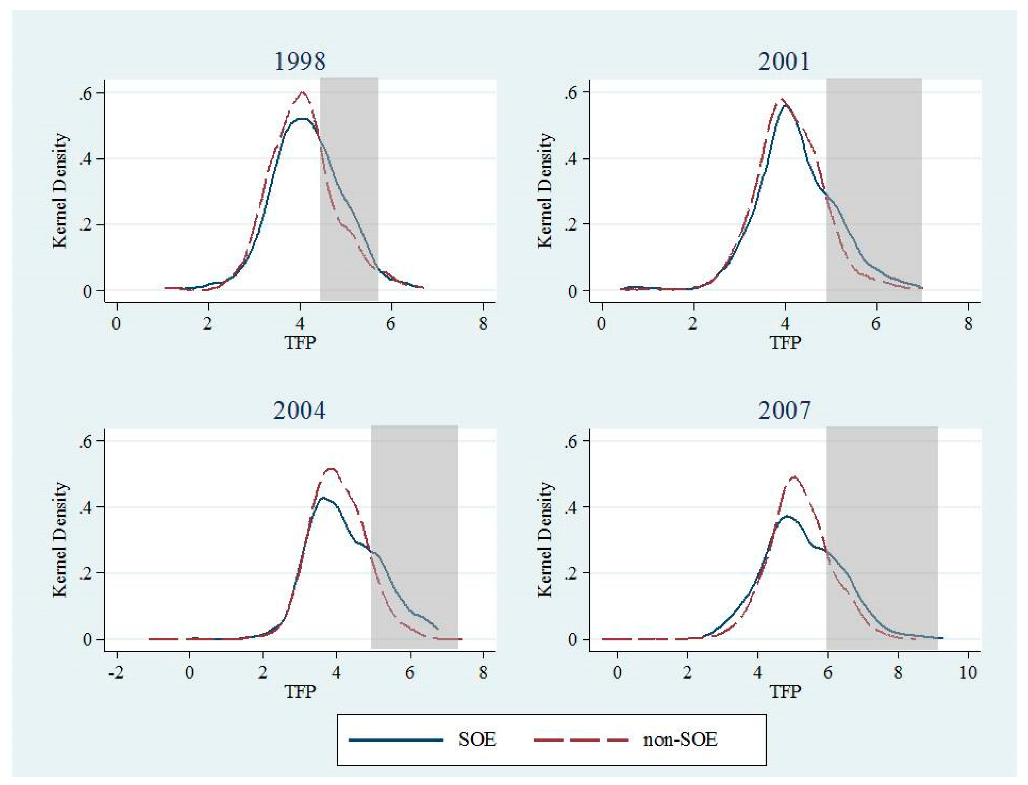
The entry and exit of non-SOE generate substantial impact on aggregate TFP changes. Unlike the manufacturing sector, most of non-state-owned entrants are small coal mines employing relatively outdated equipment. This has negative effects on aggregate TFP. Thus, SOE might have higher TFP compared to non-SOE. Figure 6 compares the TFP distribution of SOE and non-SOE for coal mining. As shown in Figure 6, TFP of non-SOE were more left-shifted, indicating lower productivity of non-SOE.

Table 5. Bonferroni test for TFP differences between SOE and non-SOE.

Row Mean Minus Column Mean	1998	2001	2004	2007
	SOE
Non-SOE	0.102 (0.038)	0.131 (0.003)	0.186 (0.000)	0.078 (0.118)

Notes: the values in brackets are p-values.

provides statistics for TFP differences between SOE and non-SOE using Bonferroni test. The SOE had higher TFP compared to non-SOE, and the differences were statistically significant at 5% level in most cases. Most of entrants induced by the coal price boom after 2003 are non-SOE, and thus the contribution of massive entry after 2003 would be negative.

The year 2007 is noteworthy; the Chinese government became devoted to enhancing coal industrial concentration in 2007, thus many coal mines were forced to exit the market. In 2007, 1249 firms exited, among them only 148 firms were state-owned while the remaining 1101 firms were non-SOE. The effect of the 2007 exit was negative, implying that the integration of coal mining industry in 2007 was not based on productivity, some non-SOE with higher productivity might have been integrated.

Then, how to interpret the rapid increase of productivity in 2007? The results in Table 3 show that it should be attributed mostly to surviving firms. Thus, we separately present the within and between firm components for surviving firms in

Table 6. The decomposition for within- and between-firm components.

	GR		FHK		DOPD
	within	between	within	between	within	between
1999	−0.0003	0.0187	−0.0583	−0.0501	−0.0141	0.0367
2000	0.0359	0.0212	−0.0008	−0.0229	0.0131	0.0623
2001	0.0151	0.0139	−0.0099	−0.0109	−0.0502	0.0947
2002	−0.0294	−0.0254	−0.0593	−0.0660	0.0010	−0.0789
2003	0.0339	−0.0066	−0.0024	−0.0411	0.0954	−0.0400
2004	0.0914	−0.0082	0.0743	−0.0298	0.1516	0.0817
2005	0.0159	−0.0367	−0.0715	−0.1186	0.0758	−0.0937
2006	0.0326	−0.0235	−0.0273	−0.0834	0.1044	−0.0916
2007	0.9001	0.0051	0.7208	−0.0760	1.0893	−0.0116

. There is no clear direction for the contributions of within and between components. Empirically, however, Table 6 shows that the rapid increase of aggregate TFP in 2007 was mainly induced by within-firm growth, rather than between-firm reallocation. This further supports that coal industry integration in 2007 was not based on productivity, which would result in growth by between-firm reallocation. On the contrary, policy intervention might distort the choice of market integration.

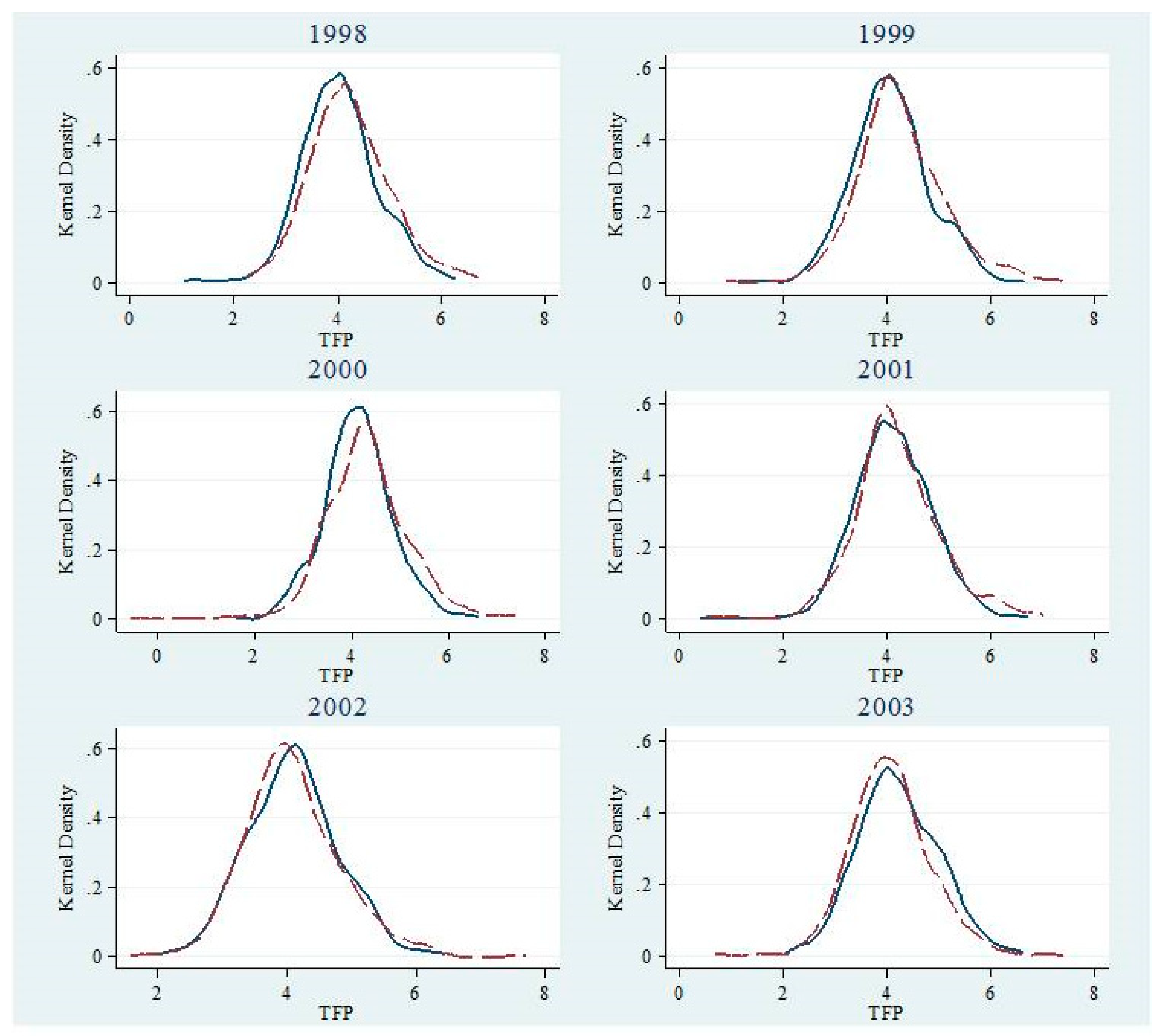
In order to further analyze the contributions of entries and exits by regions, we compared TFP distribution of MPR and non-MPR over the years, as shown in Figure 7. Interestingly, before 2003 the productivity at firm-level in non-MPR was higher than that in MPR, but the situation reversed after 2004.

We argue that the reversal might also be partly attributed to the differences of entries and exits between MPR and non-MPR.

Table 7. Number of entrants and exiters by MPR and non-MPR.

Year	Entrants		Year	Exiters
	MPR	non-MPR		MPR	non-MPR
1999	268	246	1999	53	38
2000	171	149	2000	220	155
2001	294	392	2001	386	275
2002	311	231	2002	165	135
2003	261	260	2003	328	283
2004	1512	1039	2004	435	417
2005	588	1121	2005	133	179
2006	798	907	2006	569	371
2007	69	96	2007	754	495

Notes: the bold in the column of “Entrants” in non-MPR indicates that there are much more entrants in non-MPR in 2005 and 2006; the bold in the column of “Exiters” in MPR indicates that more coal mining firms in MPR exit the market in 2007.

reports the number of entrants and exiters by MPR and non-MPR. First, the data show that there were much more entrants in non-MPR in 2005 and 2006. The massive entrants were small coal mines, which were induced by the increased coal prices. Thus, the TFP of these entrants were lower. These entrants decreased the TFP in non-MPR. Columns (1) and (2) of

Table 8. Averaged value added and TFP.

Year	Variable	Entrants in non-MPR	Non-Entrants in non-MPR	Year	Variable	Exiters in MPR	Non-Exiters in MPR
		(1)	(2)			(3)	(4)
2005	value added	26786	33875	2007	value added	47142	82696
	TFP	3.901	4.100		TFP	4.056	4.772
2006	value added	25218	34823
	TFP	3.774	4.067

support this explanation. In non-MPR, the scale of entrants was smaller than those of survivors and exiters (non-entrants) in 2005 and 2006, and the corresponding TFP was also lower. Second, more coal mining firms in MPR exit the market because of policy enforcement, and most exiters are small coal mines with lower productivity. For example, Shanxi, the largest coal production province in China, closed all firms producing less than 30 thousand tons per year in 2004; in 2006, firms producing less than 90 thousand tons per year were further forced to close. TFP in MPR gradually increased due to the exit of low productivity firms. In MPR (columns (3) and (4) of Table 8), the scale of exiters was smaller than those of entrants and survivors (non-exiters) in 2007, and the average TFP of exiters was also lower.

We further decomposed the aggregate TFP by MPR and non-MPR. The results are reported in

Table 9. The TFP decomposition for MPR and non-MPR using DOPD.

	MPR			non–MPR
	Surviving Firms	Entering Firms	Exiting Firms	Surviving Firms	Entering Firms	Exiting Firms
1999	0.0346	−0.0552	0.0253	0.0041	0.1140	0.0236
2000	0.0654	0.1586	0.0061	0.0872	0.0694	0.0392
2001	0.0566	−0.1014	0.1970	0.0233	−0.0998	0.0210
2002	−0.0991	−0.1455	0.0132	−0.0494	0.0169	−0.1185
2003	0.1004	0.1080	−0.0730	−0.0185	0.1297	−0.1076
2004	0.2717	−0.2979	0.1099	0.1663	−0.2147	0.1908
2005	−0.0300	−0.0460	0.0124	0.0102	−0.0805	−0.0009
2006	0.0487	−0.0619	0.0351	−0.0569	−0.0441	0.0673
2007	1.1261	0.0042	0.0434	0.9658	0.0927	−0.1370
	MPR			non–MPR
	within	between	net entering	within	between	net entering
1999	0.0106	0.0240	−0.0299	−0.0579	0.0620	0.1376
2000	0.0461	0.0193	0.1647	−0.0361	0.1232	0.1086
2001	−0.0147	0.0712	0.0956	−0.0996	0.1229	−0.0789
2002	0.0183	−0.1175	−0.1323	−0.0158	−0.0336	−0.1016
2003	0.1189	−0.0186	0.0350	0.0711	−0.0896	0.0221
2004	0.0947	0.1770	−0.1880	0.2084	−0.0422	−0.0239
2005	0.1215	−0.1516	−0.0336	0.0101	0.0001	−0.0813
2006	0.0676	−0.0190	−0.0268	0.1371	−0.1940	0.0232
2007	1.0523	0.0739	0.0476	1.1173	−0.1514	−0.0443

. As argued by Melitz and Polanec [4], the effects of entry and exit decomposed by GR and FHK might be biased because neither entrants in period 1 nor exiters in period 2 can be observed. To avoid redundancy, only the DOPD method was used. First, consistent with the former analysis, the contribution of exits in MPR were always positive (except for 2003), while that in non-MPR might be positive or negative. The reason is the elimination of outdated coal production capacity. Second, the integration of coal industry in 2007 generated positive effects on productivity in MPR through between-firm reallocation, but for non-MPR, the effects of between-firm reallocation were negative (between-firm reallocation contributed positively to MPR while contributed negatively to non-MPR. On average, the total effects of between-firm reallocation were negligible according to the results in Table 6.) Third, the effects of entering in non-MPR were negative in 2004, 2005, and 2006.

6. Conclusions and Policy Implications

China has been the world’s largest energy producer, and coal dominates China’s energy supply. The productivity of energy supply enhances our understanding on future energy development. Coal is the main energy source of electricity generation and the main emitter of carbon dioxide, this study would even help us make informed decisions on electricity planning and carbon cap-and-trade policies [38].

In this context, this paper investigates the productivity and its dynamic change of energy supply in China by employing the 25,627 observations of coal mining firms. We are particularly interested in the effects of entering and exiting because of the continuous entry of new firms and exit of old ones in energy supply. We find that entering and exiting of coal mining firms help explain the dynamic change of productivity. Main findings and corresponding policy implications are as follows:

First, the TFP of China’s energy supply only increases by 2.6% per year on average, which largely lags behind the growth rate of coal production. Promoting the productivity growth of China’s energy supply is significant in future development. Especially considering that labor input of unit coal production in China is still much more than that in US.

Second, the entry and exit of non-SOE partially provide explanation for the dynamic change of energy supply productivity. At firm-level, we find that SOEs usually have higher TFP than non-SOEs in coal mining sector, because most of small coal mines belongs to non-SOEs, and they tend to employ outdated equipment. The decomposition of aggregate TFP suggests that non-state owned entrants induced by the boom of coal price after 2003 have generated negative effects on the TFP of energy supply. Similarly, the exit of non-SOEs has had positive effects.

Third, the integration in 2007 aiming at enhancing coal industrial concentration has substantially stimulated the within-growth of coal mining firms. At present, the concentration ratio of China is still quite low. For example, the largest four coal mining firms in the US account for ~70% of total coal production; the largest five coal suppliers also provide more than 70% of coal in Austria. While the top ten coal mining firms only provide ~40% of China’s total production. Based on the results in this paper, promoting concentration degree of China’s coal production by industrial integration might stimulate the productivity of coal-mining firms.

Fourth, there is heterogeneity by region concerning the effects of entry and exit on energy supply productivity. More entrants, which were induced by the coal price boom after 2003, are concentrated in non-MPR, while more exiters are located in MPR due to government’s enforcement. Many entrants are small coal mines, while exiters are usually the outdated coal production capacity. Thus, the productivity of energy supply in MPR gradually surpasses that in non-MPR. From this perspective, “supply side reforms” nowadays in China might generate positive effect on energy supply productivity by restricting the entry of small coal mines and eliminating outdated coal production capacity.

References

1. Li, J.; Sun, C. Towards a low carbon economy by removing fossil fuel subsidies? China Econ. Rev. 2018, 50, 17–33. [Google Scholar] [CrossRef]
2. British Petroleum. Statistical Review of World Energy 2018; BP: London, UK, 2018. [Google Scholar]
3. Brandt, L.; Van Biesebroeck, J.; Zhang, Y. Creative accounting or creative destruction? Firm-level productivity growth in Chinese manufacturing. J. Dev. Econ. 2012, 97, 339–351. [Google Scholar] [CrossRef] [Green Version]
4. Melitz, M.J.; Polanec, S. Dynamic Olley-Pakes productivity decomposition with entry and exit. RAND J. Econ. 2015, 46, 362–375. [Google Scholar] [CrossRef] [Green Version]
5. Van Beveren, I. Total factor productivity estimation: A practical review. J. Econ. Surv. 2012, 26, 98–128. [Google Scholar] [CrossRef]
6. Oberfield, E. Productivity and misallocation during a crisis: Evidence from the Chilean crisis of 1982. Rev. Econ. Dyn. 2013, 16, 100–119. [Google Scholar] [CrossRef]
7. Kalirajan, K.P.; Obwona, M.B.; Zhao, S. A decomposition of total factor productivity growth: The case of Chinese agricultural growth before and after reforms. Am. J. Agric. Econ. 1996, 78, 331–338. [Google Scholar] [CrossRef]
8. Kim, S.; Han, G. A decomposition of total factor productivity growth in Korean manufacturing industries: A stochastic frontier approach. J. Prod. Anal. 2001, 16, 269–281. [Google Scholar] [CrossRef]
9. Menegaki, A.N. Growth and renewable energy in Europe: Benchmarking with data envelopment analysis. Renew. Energy 2013, 60, 363–369. [Google Scholar] [CrossRef]
10. Van Biesebroeck, J. Robustness of productivity estimates. J. Ind. Econ. 2007, 55, 529–569. [Google Scholar] [CrossRef]
11. Syverson, C. What determines productivity? J. Econ. Lit. 2011, 49, 326–365. [Google Scholar] [CrossRef]
12. Syverson, C. Challenges to mismeasurement explanations for the US productivity slowdown. J. Econ. Perspect. 2017, 31, 165–186. [Google Scholar] [CrossRef]
13. Menegaki, A.N. The Economics and Econometrics of the Energy-Growth Nexus; Academic Press: Cambridge, MA, USA, 2018. [Google Scholar]
14. Yasar, M.; Raciborski, R.; Poi, B. Production function estimation in Stata using the Olley and Pakes method. Stat. J. 2008, 8, 221–231. [Google Scholar] [CrossRef]
15. Olley, S.; Pakes, A. The dynamics of productivity in the telecomunications equipment industry. Econometrica 1996, 64, 1263–1297. [Google Scholar] [CrossRef]
16. Amiti, M.; Konings, J. Trade liberalization, intermediate inputs, and productivity: Evidence from Indonesia. Am. Econ. Rev. 2007, 97, 1611–1638. [Google Scholar] [CrossRef]
17. Fan, H.; Li, Y.A.; Yeaple, S.R. On the relationship between quality and productivity: Evidence from China’s accession to the WTO. J. Int. Econ. 2018, 110, 28–49. [Google Scholar] [CrossRef]
18. Boeing, P.; Mueller, E.; Sandner, P. China’s R&D explosion—Analyzing productivity effects across ownership types and over time. Res. Policy 2016, 45, 159–176. [Google Scholar]
19. Aghion, P.; Cai, J.; Dewatripont, M.; Du, L.; Harrison, A.; Legros, P. Industrial Policy and Competition. Am. Econ. J. Macroecon. 2015, 7, 1–32. [Google Scholar] [CrossRef] [Green Version]
20. Hsieh, C.T. Policies for Productivity Growth. Global Dialogue on the Future of Productivity Growth: Towards an OECD Productivity Network. Mexico City. 2015, pp. 1–15. Available online: https://www.oecd.org/eco/growth/Policies%20for%20productivity%20growth_Chang%20Tai%20Hsieh.pdf (accessed on 21 July 2018).
21. Harrison, A.E.; Martin, L.A.; Nataraj, S. Learning versus stealing: How important are market-share reallocations to India’s productivity growth? World Bank Econ. Rev. 2013, 27, 202–228. [Google Scholar] [CrossRef]
22. Arnold, J.M.; Javorcik, B.S.; Mattoo, A. Does services liberalization benefit manufacturing firms?: Evidence from the Czech Republic. J. Int. Econ. 2011, 85, 136–146. [Google Scholar] [CrossRef]
23. Zhang, C.; Liu, H.; Bressers, H.T.A.; Buchanan, K.S. Productivity growth and environmental regulations-accounting for undesirable outputs: Analysis of China’s thirty provincial regions using the Malmquist–Luenberger index. Ecol. Econ. 2011, 70, 2369–2379. [Google Scholar] [CrossRef]
24. Chen, S.; Golley, J. ‘Green’ productivity growth in China’s industrial economy. Energy Econ. 2014, 44, 89–98. [Google Scholar] [CrossRef]
25. Liu, H.; Li, J.; Long, H.; Li, Z.; Le, C. Promoting energy and environmental efficiency within a positive feedback loop: Insights from global value chain. Energy Policy 2018, 121, 175–184. [Google Scholar] [CrossRef]
26. Shao, S.; Luan, R.; Yang, Z.; Li, C. Does directed technological change get greener: Empirical evidence from Shanghai’s industrial green development transformation. Ecol. Indic. 2016, 69, 758–770. [Google Scholar] [CrossRef]
27. Li, J.; Lin, B. Green economy performance and green productivity growth in China’s cities: Measures and policy implication. Sustainability 2016, 8, 947. [Google Scholar] [CrossRef]
28. Lin, B.; Du, K. Modeling the dynamics of carbon emission performance in China: A parametric Malmquist index approach. Energy Econ. 2015, 49, 550–557. [Google Scholar] [CrossRef]
29. Darmstadter, J.; Kropp, B. Productivity Changes in US Coal Mining; Resources for the Future: Washington, DC, USA, 1997. [Google Scholar]
30. Bradley, C.; Sharpe, A. A Detailed Analysis of the Productivity Performance of Mining in Canada; Centre for the Study of Living Standards: Ottawa, ON, Canada, 2009. [Google Scholar]
31. Kwoka, J.; Pollitt, M. Do mergers improve efficiency? Evidence from restructuring the US electric power sector. Int. J. Ind. Organ. 2010, 28, 645–656. [Google Scholar] [CrossRef]
32. Okazaki, T. Productivity change and mine dynamics: The coal industry in Japan during World War II. Jahrbuch für Wirtschaftsgeschichte/Econ. Hist. Yearbook 2014, 55, 31–48. [Google Scholar] [CrossRef]
33. Zhang, D.; Cao, H.; Dickinson, D.G.; Kutan, A.M. Free cash flows and overinvestment: Further evidence from Chinese energy firms. Energy Econ. 2016, 58, 116–124. [Google Scholar] [CrossRef]
34. Baily, M.N.; Hulten, C.; Campbell, D. Productivity dynamics in manufacturing plants. Brookings Papers on Economic Activity. Microeconomics 1992, 1992, 187–267. [Google Scholar]
35. Griliches, Z.; Regev, H. Firm productivity in Israeli industry 1979–1988. J. Econ. 1995, 65, 175–203. [Google Scholar] [CrossRef]
36. Foster, L.; Haltiwanger, J.C.; Krizan, C.J. Aggregate Productivity Growth. Lessons from Microeconomic Evidence. Lessons from Microeconomic Evidence; NBER Chapters; University of Chicago Press: Chicago, IL, USA, 2001; pp. 303–372. [Google Scholar]
37. Nie, H.; Jiang, T.; Yang, R. A Review and Reflection on the Use and Abuse of Chinese Industrial Enterprises Database. World Economy. (in Chinese). 2012, pp. 142–158. Available online: https://papers.ssrn.com/sol3/papers.cfm?abstract_id=2323998 (accessed on 28 October 2018).
38. Hong, S.; Sim, S.G. Inelastic supply of fossil energy and competing environmental regulatory policies. Sustainability 2018, 10, 287. [Google Scholar] [CrossRef]
Figure 1. Trends of energy demand and production in several countries (2000–2017). (a) Comparison of energy demand. (b) Comparison of energy supply.
Sustainability 11 00983 g001
Figure 2. The ratio of output to the number of workers in the coal mining industry. (The unit is thousand ton per worker. The left axis is the labor productivity for China, while the right axis is the labor productivity for the US).
Sustainability 11 00983 g002
Figure 3. Total number of firms, entrants and exiters by regions. (a) Number of coal mining firms in MPR and non-MPR; (b) number of entrants in MPR and non-MPR; and (c) number of exiters in MPR and non-MPR.
Sustainability 11 00983 g003
Figure 4. The distribution of TFP at firm-level by year.
Sustainability 11 00983 g004
Figure 5. Aggregate TFP during 1998 and 2007.
Sustainability 11 00983 g005
Figure 6. The TFP distribution by ownership types. (The shadow areas indicate that more SOEs are distributed in this interval.).
Sustainability 11 00983 g006
Figure 7. The distribution of TFP in MPR and non-MPR.
Sustainability 11 00983 g007aSustainability 11 00983 g007b