Energy and Environmental Efficiency in Different Chinese Regions

Abstract

China has become the second-largest economy in the world; however, the price of its rapid economic development has been a rise in serious environmental pollution, with air quality being a major public issue in many regions. However, few previous energy and environmental sustainability studies have included the Air Quality Index (AOI) and in particular CO₂ and PM_2.5 emissions in their calculations and few have included regional differences, as these are difficult to describe using radial and non-radial methods. In this paper, DEA (Data Envelopment Analysis) is used to assess the energy and economic efficiencies of Chinese provinces and cities, in which the environmental pollution source variable is CO₂, and the main methods applied are radial (CCR or BCC) and non-radial SBM (Slacks Based Measures). Different from past studies, this study used both a Meta Undesirable EBM (Epsilon-Based measure) method to overcome the radial and non-radial errors and geographical differences and AQI environmental pollution indicators to accurately assess the economic, energy, and environmental efficiencies. It was found that: (1) Guangzhou and Shanghai had the best four-year efficiencies, (2) the energy efficiency differences in each city were large and there was a significant need for improvements, (3) the GDP efficiencies in each city were high, indicating that all cities had strong economic development, (4) the CO₂ efficiencies indicated that around half the cities had had sustained improvements, (5) the AQI efficiencies in each city were low and there was a significant need for improvement, and (6) the technological differences between the cities were large, with the efficiencies in the high-income cities being much higher than in the low-income cities.

1. Introduction

From 2010 to 2015, China’s GDP output grew at an annual rate of 8%, and even though it declined in 2015, it managed to achieve an annual growth of 6%. By 2016, China’s GDP was around 18% of the global GDP [1]. Most of China’s economic growth was due to growth in the industrial sector, with coal and electrical energy being the main engines for GDP growth. However, the rise in the industrial and manufacturing sectors has had an adverse impact on China’s environment, and it is now the largest global carbon dioxide emitter, with three-quarters of Chinese cities failing to meet domestic air quality standards [1]. In the 2015 Paris Agreement, China set a target of a 60–65% reduction in carbon dioxide emissions by 2030 from 2005 levels. The “13th Five-Year Ecological Environmental Protection Plan” (2016–2020), which was formulated in 2016, set a target of 80% “good” air quality in 338 major cities by 2020. Although many measures have been taken to limit carbon dioxide emissions; regional economies, populations, and resources vary widely, with the energy demands in each region being quite different. For example, the coastal industrial provinces in the eastern region have higher energy demands than the western provinces. Therefore, it is vital to track the economic, energy and environmental performances in the various regions so as to be able to sustain economic growth, while reducing $C{O}_2$ and $P{M}_{2.5}$ emissions.

Some previous energy and environmental research works have focused on energy or environmental efficiency [2,3,4,5,6,7,8,9,10,11,12,13,14], some have focused on the factors affecting energy efficiency [15,16,17,18,19,20,21,22], some have explored the environmental impacts of $C{O}_2$ emissions [23,24,25,26] and some have considered $S{O}_2$, $N{O}_2$ or other pollutants as the undesirable outputs for energy and environmental efficiency assessments [27,28,29,30,31,32,33].

These earlier analyses were usually based on radial (CCR or BCC), non-radial (SBM) or Directional Distance function models; however, these three models have been known to over and/or underestimate the efficiency values. The other disadvantage of the above studies was that each city was considered homogeneous; however, this type of research approach is not suitable for countries with large regional differences like China, as significant biases could occur during the efficiency evaluations. Past research has also only tended to evaluate the efficiencies of $C{O}_2$ and energy, but has not considered other pollution indicators. This paper, therefore, considers other air pollutants and adopts a meta-undesirable EBM DEA model to explore the energy and economic efficiencies in 31 cities in China.

This paper makes three main contributions. First, in past Chinese regional (city or province) comparisons, the inputs were labor, capital and energy, the desirable output was GDP, and the undesirable output was $C{O}_2$ or $S{O}_2$; however, other pollutants were omitted. This paper considers not only $C{O}_2$ but also the AQI, which includes particulate matter ($P{M}_{2.5}$ and $P{M}_{10}$), sulfur dioxide ($S{O}_2$), ozone ($O_3$), and carbon monoxide ($CO$). Second, past research methods have used radial (CCR and BCC), non-radial (SBM), and Directional Distance function models, all of which ignore either the radial or non-radial characteristics, which tends to result in biased results. This paper use a meta-undesirable EBM DEA model to overcome these shortfalls. Third, past research has treated each region in China as homogeneous; however, as each region has different resource endowment and income levels, this paper separates the provinces and cities into high income regions and upper-middle income regions to explore the regional differences. Data from 2013 to 2016 in 31 cities in China were extracted for the analysis, with labor, fixed assets and energy consumption being the inputs, GDP being the good output, and $C{O}_2$ and the AQI being the bad outputs.

The remainder of this paper is organized as follows. Section 2 presents the literature review, Section 3 describes the research method, Section 4 gives the empirical results and the discussion, and Section 5 gives the conclusions and policy recommendations

2. Literature Review

Energy and environmental efficiency research has tended to follow three main directions: comparisons of energy and environmental efficiencies, energy efficiency factor analyses, and air pollutant effects ($C{O}_2$, $S{O}_2$, $N{O}_2$) on the environment.

Hu and Wang [2] used a Radial DEA model to analyze China’s energy efficiency and explore the relationship between China’s economic growth and energy efficiency improvements. Fang et al. [3] used DEA to explore energy efficiency in China and the United States, finding that Chinese companies had lower technical efficiencies than American companies. Shi et al. [4] explored regional energy efficiency in China, and found that the energy efficiencies in the eastern regional industries were better than the energy efficiencies in the western regional industries. Li and Hu [5] calculated the ecological total-factor energy efficiency (ETFEE) of 30 regions in China from 2005 to 2009 using an SBM model, and found that the regional ETFEE was at a relatively low level of around 0.600; regional energy efficiency exceeded 0.100, did not consider the environmental impact, and was extremely uneven, with the eastern regions being significantly better than the western regions, and with the truncated regression model showing that R&D spending had a positive impact on GDP and foreign dependence. Zhang and Choi [6] used an SBM DEA model to study the environmental efficiencies in various provinces in China, finding that most provinces had low energy efficiency. Wang and Wei [7] used SBM models to assess energy, economic, and environmental efficiencies, and found that while China’s economy was performing well, the energy and environmental efficiencies were poor, technological progress was a major factor in productivity growth, and declines in scale and management efficiency were the two major obstacles to productivity. Liu and Wang [8] claimed that China’s energy conservation and emissions reduction processes required a specific and accurate assessment of the energy efficiency of the industrial sector, as this accounted for 70% of China’s total energy consumption. Previous research has used DEA (Data Envelopment Analysis) models to calculate the energy efficiency without regard for the internal structure of the industrial sector, which could cause biased results because of the “black box” assessment. By separating the energy production sector from the energy consumption sector, a network DEA model can be used to assess the energy efficiency of China’s provincial industrial sectors.

Pang et al. [9] use SBM DEA to analyze the efficiency of 87 countries and found that European countries were more efficient in reducing emissions and increasing energy efficiency. Apergis et al. [10] studied the energy efficiency in OECD countries, finding that capital-intensive OECD countries were more efficient than labor-intensive countries. Guo et al. [14] used a dynamic SBM DEA method to research the energy efficiencies in 26 OECD countries, and found that Canada and China had the best energy efficiencies. Geng et al. [11] used a DEA cross-model (DEACM) to analyze the energy and environmental efficiencies by dividing the inputs into energy and non-energy inputs, and the outputs into expected and undesired outputs, from which it was found that the environmental improvement DEACM method was more effective than the original DEA method in analyzing the energy and environmental efficiencies of ethylene production in complex chemical processes. Hu et al. [13] used a congestion total-factor energy efficiency model to analyze four energy sources and the energy efficiencies in 20 administrative Taiwanese regions from 2004 to 2013, finding that Taipei City, Taitung County, and Peng-hu County did not experience excessive energy input over the entire period, and that Taiwan’s energy efficiencies were related to its regional development characteristics; for example, such as the natural, green and environmentally friendly tourist areas in Taitung County and Peng-hu County. Du et al. [12] conducted a cross-provincial comparison of China’s carbon dioxide emissions from 2006 to 2012, and found that economic activity (EAT) was the main reason for the increased emissions, while changes in potential energy intensity (PEI), energy structure change (EMX) and efficiency change (EC) could reduce $C{O}_2$ emissions in most provinces/cities in China.

In energy efficiency analyses, Martinez and Silveira [15] found that higher energy taxes, electricity consumption, investment and labor productivity were able to improve the energy efficiency of Swedish industry. Lu et al. [16] use DEA and Tobit Regression models to research China’s energy efficiency, finding that industrial structure, energy consumption structure, and institutional factors had a significant impact on energy efficiency. Li et al. [17] used the DEA-Malmquist method to explore China’s energy efficiency, and found that technological reforms had a negative impact on energy intensity. Lin and Yang [18] explored the energy efficiency of power companies, finding that foreign capital was conducive to improving the energy efficiency in power companies. Lin and Liu [19] found that urbanization had contributed to the increase in $C{O}_2$ emissions in China, and that using less energy was a major factor in reducing $C{O}_2$ emissions. Feng et al. [22] used DEA to explore energy efficiency and $C{O}_2$ reduction factors in various provinces of China, and found that there were three main reasons obstructing $C{O}_2$ emissions reductions; structural inefficiencies, technology inefficiencies, and management inefficiencies. Jebali et al. [20] used a double bootstrap DEA to research the energy efficiencies in Mediterranean countries from 2009–2012 and found that while the overall energy efficiencies were high, they were declining over time, and that per capita GNI, population density, and renewable energy use could affect energy efficiency. Li and Boqiang [21] proposed a total-factor energy consumption performance index (TEPI) to measure the energy efficiencies of 30 provinces in China from 1997 to 2012. Using a two-stage double bootstrap approach, it was found that China’s technological energy innovations had a negative impact on TEPI, and that the introduction of technology and imitation innovation had a positive impact on TEPI, with TEPI improvements being found to come mainly from technological introductions, and that foreign direct investment (FDI) had an important effect on imitation innovation and was able to improve China’s energy efficiency.

In assessments on the environmental impacts of $C{O}_2$ emissions, Ang and Zhang [23] examined the differences between global $C{O}_2$ emissions and $C{O}_2$ emissions per capita, Zofil and Priteo [24] used DEA to assess the relative efficiency of manufacturing in 14 OECD countries and found that undesirable $C{O}_2$ emissions output had an adverse impact, and Sueyoshi and Goto [25] used data envelopment analysis and the Marquist Productivity Index to explore the relationships between mixed fuel energy, electricity, and carbon dioxide in 10 industrial countries and their respective impacts on environmental output. Chansarn [26] evaluated the efficiency of 115 high- and middle-income countries, with carbon dioxide emissions as undesirable output, finding that Croatia, Hong Kong, Hungary, Israel, Malta, Poland, Portugal, Sweden, and Switzerland were using less resources to achieve maximum efficiency and therefore had less impact on the environment. Zhou et al. [27] used non-radial DEA to assess environmental efficiency, with the desirable output being GDP, and the undesirable outputs being $C{O}_2$ emissions, $N{O}_X$ emissions, $S{O}_X$ emissions, and $CO$ emissions. Sozen et al. [28] used DEA to assess the operations and environmental efficiencies of 15 thermal power plants in Turkey and used $C{O}_2$ emissions, $S{O}_2$ emissions, $N{O}_2$ emissions, and other gas emissions to assess thermal power generation efficiency. Tsolas [29] explored the production efficiencies of fossil fuel power plants in Greece, with net power as the desirable output, and sulfur dioxide $S{O}_2$, nitrogen oxides $N{O}_X$, and carbon dioxide $C{O}_2$ as the undesirable outputs. Yang et al. [30] assessed urban sustainability with pollution as the undesirable output to measure the input-output efficiency of Taiwan’s 22 administrative regions, finding that Taipei City and Lianjiang County were the most sustainable cities, the industrial structure had a significant impact on resource efficiency and pollution efficiency, and that Taiwan needed to improve its electricity and water efficiencies. Yang et al. [31] used an SBM model to evaluate the combined heat and power (CHP) of 31 Chinese eco-industrial parks, with the inputs being coal consumption, freshwater consumption, capital depreciation, and operating costs, and the outputs being electricity, heat, and greenhouse gas emissions. The eco- and thermal efficiencies at the CHP plants were found to be very different, and the annual working hours were found to be the most important factors affecting eco-efficiency. Qin et al. [32] dynamically assessed the energy efficiencies in China’s coastal areas from 2000 to 2012 using a global Malmquist-Luenberger Productivity Index and found that these regions had the following characteristics: (1) the economic development level was positively correlated with energy efficiency performance; (2) except for Beijing and Hainan, energy efficiency performances declined when the undesirable output was considered; (3) the energy efficiency of the Bohai Economic Zone had improved; and (4) the main obstacles to energy efficiency were technological improvements, scale efficiency, and management. Guo et al. [33] assessed the coal consumption efficiencies of six energy-intensive industries in China in 2015, with sulfur, carbon dioxide, nitrogen oxides and industrial fumes, and dust and soot emissions being the undesirable outputs, and found that there were two energy-intensive industries with higher coal economic efficiency than coal environmental efficiency, concluding that China should pay more attention to green coal energy use and that highlighting economic benefits over environmental impacts tended to obscure the negative environmental impacts.

Some environmental research has focused on specific issues. Wang et al. [34] used an SBM, window analysis and a panel Tobit regression to assess carbon emissions efficiencies in China from 2003 to 2016 (11th Five-Year Plan), finding that resource quantity, abatement potential, and resource dependence all affected carbon emissions. Li et al. [35] investigated the relationships between natural resources, manufacturing structures, and carbon emissions in China from 2003–2014, and found that resource dependence and industrialization could positively influence emissions reductions. Ji et al. [36] examined 18 top European electricity companies and explored the interdependence of carbon price and electricity stock returns. Zhang et al. [37] calculated the energy intensity in China and found that the rate was decreasing. Ma et al. [38] examined the fog and haze in 152 cities in China, finding that emissions in China were consistent with the Environmental Kuznets Curve (EKC) and that air pollutants were specifically associated with economic development. Xian et al. [39] conducted a scenario analysis on carbon emissions reductions in China from 2016–2020 and provided policy suggestions. Han et al. [40] examined 89 “Belt and Road” (BR) countries, finding that that trade and regional cooperation improved overall energy efficiency.

More recently, a Directional Distance Function (DDF) approach was used in environmental research. For example, Riccardi et al. [41] analyzed cement industry emissions in 21 countries using three DEA methods (CCR, BCC, DDF). Wang et al. [42] estimated firm energy performances and technology gaps in Guangdong using a meta-frontier DDF. DDF has also been used in cost abatement analyses [43,44,45]. Of the above research approaches, CCR and BCC model are radial models and the DDF model is able to separately conduct both radial and non-radial analysis separately; therefore, as there is as yet no model that can deal with both radial and non-radial analyses, in this paper, a meta–undesirable EBM DEA model is designed to account for both the radial and non-radial models.

Chinese regional economic and environmental differences and other air pollutants are considered in the meta–undesirable EBM DEA model in this paper to explore the energy and economic efficiencies in 31 Chinese cities.

3. Research Method

DEA was first proposed by Farrell [46] in 1957, after which Charnes et al. [47] developed the main theoretical CCR model. Banker et al. [48] then expanded the assumptions on the returns to scale and proposed BCC models for Technical Efficiency (TE) and Scale Efficiency (SE), both of which were able to measure radial efficiency and in which the inputs and outputs were assumed to proportionally increase or decrease. Tone [49] then proposed a non-radial Slacks-Based Measure that was able to account for both input slacks and the differences in the terms on a single scalar SBM 0 to 1 efficiency scale. Directional Distance Function (DDF) uses a directional function to analyze DMU efficiency, and as the directional input and output vectors indicate the relative importance, DDF is therefore able to effectively coordinate the undesirable output variables in the model ([50]), which means that for any given input, the desirable output can be increased and the undesirable output decreased. Cooper et al. [51] also included undesirable output in an SBM model. However, as both the CCR and BCC are radial DEA models, they ignore the non-radial slacks when evaluating efficiency values, and the SBM, which is a non-radial DEA model, fails to consider the characteristics of the radial model. To resolve these shortcomings, Tone and Tsutsui [52] proposed the EBM (Epsilon-Based Measure) DEA model.

Non-Oriented EBM

With $n$ $DMU$, where $DM{U}_j=\left(DM{U}_1,DM{U}_2,\dots ,DM{U}_k,\dots ,DM{U}_n\right)$. $m$ kinds of inputs $X_j=\left(X_{1j},X_{2j},\dots ,X_{mj}\right)$, and $s$ outputs $Y_j=\left(Y_{1j},Y_{2j},\dots ,Y_{sj}\right)$, the efficiency value of $DMU$:

$$K^{*}=\underset{0,\eta ,\lambda ,s^{-},s^{+}}{\min }\frac{\theta -{\mathsf{\epsilon }}_x{{\displaystyle \sum }}_{i=1}^m\frac{w_i^{-}{s}_i^{-}}{x_{i0}}}{\eta +{\mathsf{\epsilon }}_y{{\displaystyle \sum }}_{i=1}^s\frac{w_i^{+}{s}_i^{+}}{y_{i0}}}$$

$$\mathrm{Subject}\mathrm{to}\mathsf{\theta }{X}_0-X_{\lambda }-S^{-}=0$$

(1)

• $\eta Y_0-Y_{\lambda }+S^{+}=0,$
• ${\lambda }_1+{\lambda }_2+\dots +{\lambda }_n=1$
• $\lambda \ge 0,S^{-}\ge 0,S^{+}\ge 0.$
• Y: DMU output,
• X: DMU input,
• $S^{-}$: Slack variable,
• $S^{+}$: Surplus variable,
• $W^{-}$: Weight of the input $\mathrm{I}$, ${{\displaystyle \sum }}^{}{W}_i^{-}=1\left({\forall }_i{W}_i^{-}\ge 0\right)$,
• $W^{+}$: Weight of the output S, ${{\displaystyle \sum }}^{}{W}_i^{+}=1\left({\forall }_i{W}_i^{+}\ge 0\right)$,
• ${\epsilon }_x$: Set of radial $\mathsf{\theta }$ and non-radial slacks,
• ${\epsilon }_y$: Set of radial $\eta$ and non-radial slacks.

3.1. Empirical Model for This Study: Modified Meta Undesirable EBM DEA Model

As Tone and Tsutsui’s [52] EBM model did not consider undesirable factors or regional differences, based on the EBM DEA, the meta frontier, and the undesirable factors, this paper proposes a modified meta-free EBM DEA model to evaluate the energy, economy, CO₂, and AQI efficiencies in 31 cities in China.

The modified meta unwanted EBM DEA model is described in the following:

Traditional DEA usually assumes that all producers have the same level of production technology; however, decision-making units often have different production technologies because of different management types, resources, regulations, or environmental situations. Battese and Rao [53], Battese et al. [54], and O’Donnell et al. [55] applied the meta-frontier concept to efficiency estimations to estimate the meta-frontier of all samples, then grouped the decision-making units to estimate the group frontier for each individual group. Finally, the distance between the meta-frontier and the group frontier was used to assess the level of production technology in the group sample.

$N$ firms are composed of the DMU groups (N = N₁ + N₂ +…+ N_G), x_ij and y_rj are the inputs, i (i = 1, 2, …, m) and the final output is r (r = 1, 2, …, S) for the unit j (j = 1, 2, …, N). Under the meta-frontier, the output weight $u_{\mathrm{r}}^{\mathrm{g}}$ (r = 1, 2, …, S) can be used to reach optimal efficiency, and the efficiency under the meta-frontier can be determined using the following linear programming procedure.

Meta UNDESIRABLE EBM

$$\underset{o\eta \lambda s^{-}{s}^{+}}{\min }\frac{\theta -{\epsilon }_x{{\displaystyle \sum }}_{g=1}^G{{\displaystyle \sum }}_{i=1}^m\frac{W_i^{-}{S}_i^{-}}{X_{i0}}}{\eta -{\epsilon }_y[{{\displaystyle \sum }}_{g=1}^G{{\displaystyle \sum }}_{i=1}^{S1}\frac{w_i^{+S1}{s}_i^{+goood}}{y_{i0}}+{{\displaystyle \sum }}_{g=1}^G{{\displaystyle \sum }}_{i=1}^{S2}\frac{w_i^{-S2}{s}_i^{-bad}}{y_{i0}}]}$$

Subject to

$$X_{i0}={\displaystyle \sum }_{g=1}^G{\displaystyle \sum }_{j=1}^n{X}_{ijg}{\theta }_{jg}-S_i^{-}\left(i=1\dots m\right)$$

$$Y_{i0}={\displaystyle \sum }_{g=1}^G{\displaystyle \sum }_{j=1}^n{Y}_{ijg}{\eta }_{jg}+S_i^{+good}\left(i=1\dots s1\right)$$

$$Y_{i0}={\displaystyle \sum }_{g=1}^G{\displaystyle \sum }_{j=1}^n{Y}_{ijg}{\eta }_{jg}-S_i^{-bad}\left(i=1\dots s2\right)$$

$${\displaystyle \sum }_{g=1}^G{\displaystyle \sum }_{j=1}^n{\lambda }_{jg}=1$$

(2)

• $\lambda \ge 0,S^{-}\ge 0,S^{+good}\ge 0,S^{-bad}\ge 0$, $\theta \le 1$, $\eta \ge 1$
• Y: DMU output,
• X: DMU input,
• $S^{-}$: Slack variable,
• $S^{+good}$ Surplus variable,
• $S^{-bad}$: Surplus variable,
• $W^{-}$: Weight of the input i, ${{\displaystyle \sum }}^{}{W}_i^{-}=1\left({\forall }_i{W}_i^{-}\ge 0\right)$
• $W^{+}$: Weight of output S, ${{\displaystyle \sum }}^{}{W}_i^{+S1}+{{\displaystyle \sum }}^{}{W}_i^{-S2}=1\left({\forall }_i{W}_i^{+}\ge 0\right)$
• ${\epsilon }_x$: Set of radial $\mathsf{\theta }$ and non-radial slack,
• ${\epsilon }_y$: Set of radial $\eta$ and non-radial slack.

From the above equations, the overall technological efficiency of all cities can be determined under the meta-frontier. Using Equation (2), the overall technological efficiency of all high-income and upper-middle income cities can be determined under the meta-frontier.

Undesirable EBM group meta-frontier model

The high income and upper-middle income cities are divided into decision-making units, each of which chooses an optimal output weight. The efficiency is then determined as shown in the following model:

$$\underset{o\eta \lambda s^{-}{s}^{+}}{\min }\frac{\theta -{\epsilon }_x{{\displaystyle \sum }}_{i=1}^m\frac{W_i^{-}{S}_i^{-}}{X_{i0}}}{\eta -{\epsilon }_y{{\displaystyle \sum }}_{i=1}^{S1}\frac{w_i^{+S1}{s}_i^{+goood}}{y_{i0}}+{{\displaystyle \sum }}_{i=1}^{S2}\frac{w_i^{-S2}{s}_i^{-bad}}{y_{i0}}]}$$

Subject to

$$X_{i0}={\displaystyle \sum }_{j=1}^n{X}_{ij}{\theta }_j-S_i^{-}\left(i=1\dots m\right)$$

$$Y_{i0}={\displaystyle \sum }_{j=1}^n{Y}_{ij}{\eta }_j+S_i^{+goood}\left(i=1\dots s1\right)$$

$$Y_{i0}={\displaystyle \sum }_{j=1}^n{Y}_{ij}{\eta }_j-S_i^{-bad}\left(i=1\dots s2\right)$$

$${\displaystyle \sum }_{j=1}^n{\lambda }_j=1$$

(3)

$$\lambda \ge 0,S^{-}\ge 0,S^{+good}\ge 0,S^{-bad}\ge 0,\theta \le 1,\eta \ge 1$$

Technology gap ratio (TGR)

The ratio of the overall meta-frontier and the group meta-frontier is called the Technology Gap Ratio (TGR), which is calculated as follows:

$$\mathrm{TGR}=\frac{{\mathsf{\rho }}^{*}}{{\mathsf{\rho }}_0^{*\mathrm{g}}}$$

(4)

3.2. Urban Energy, Environmental, CO₂, AQI, and GDP Efficiencies

Based on the total-factor energy efficiency in Hu and Wang [2], the energy efficiency is analyzed using an economic production function model and DEA, with economic productivity, labor, capital and energy as the inputs, and GDP as the output. Energy consumption can be reduced to an optimal level (most efficient) when GDP is increasing. In the DEA framework, energy efficiency is estimated from the distance between energy consumption and the efficiency frontier.

DEA uses linear programming to estimate the efficiencies of the decision-making units (DMU). When a DMU’s efficiency is on the DEA efficiency frontier, the DMU is efficient; otherwise, the DMU is not efficient. Therefore, the project point on the frontier is the goal of inefficient DMUs. The calculation method to determine the target input and output is as follows:

Target value = original value + adjustment value

For the adjustment value, the input must be reduced and the output increased to reach optimal efficiency. For the energy input, the “target energy level” is the optimal energy consumption efficiency. Therefore, the energy consumption adjustment value is the distance between the target value and the original value, and also reflects the actual energy consumption inefficiency; the definition for which is as follows:

$$\mathrm{Total}-\mathrm{factor}\mathrm{energy}\mathrm{efficiency}=\frac{\mathrm{Target}\mathrm{energy}\mathrm{input}\left(\mathrm{i},\mathrm{t}\right)}{\mathrm{Actual}\mathrm{energy}\mathrm{input}\left(\mathrm{i},\mathrm{t}\right)}$$

Due to a lack of target and actual pollution comparisons, Li and Hu [5] designed the following index:

$$\mathrm{Ecological}\mathrm{total}-\mathrm{factor}\mathrm{pollution}\mathrm{efficiency}\mathrm{index}=\frac{\mathrm{Target}\mathrm{pollution}\left(\mathrm{i},\mathrm{t}\right)}{\mathrm{Actual}\mathrm{pollution}\left(\mathrm{i},\mathrm{t}\right)}$$

In line with Hu and Wang [2], a total-factor energy efficiency index was used to overcome any possible bias in the traditional energy efficiency indicators. There are four key features in this study: energy efficiency, CO₂ efficiency, AQI efficiency, and GDP efficiency. In this study, i represents area and t represents time.

Input: Energy efficiency

The energy efficiency is the ratio of the target energy input to the actual energy input:

$$\mathrm{Energy}\mathrm{efficiency}=\frac{\mathrm{Target}\mathrm{energy}\mathrm{input}\left(\mathrm{i},\mathrm{t}\right)}{\mathrm{Actual}\mathrm{energy}\mathrm{input}\left(\mathrm{i},\mathrm{t}\right)}$$

When the target energy input is judged as efficient, it is equal to the actual input level and the energy efficiency equals 1. When the target energy input is less than the actual input level, the energy efficiency is less than 1, indicating some degree of inefficiency.

Undesirable Output: CO₂ efficiency

The CO₂ efficiency is the ratio of the target undesirable CO₂ output to the actual undesirable CO₂ output:

$${\mathrm{CO}}_2\mathrm{efficiency}=\frac{\mathrm{Target}{\mathrm{CO}}_2\mathrm{Undesirable}\mathrm{output}\left(\mathrm{i},\mathrm{t}\right)}{\mathrm{Actual}{\mathrm{CO}}_2\mathrm{Undesirable}\mathrm{output}\left(\mathrm{i},\mathrm{t}\right)}$$

When the target CO₂ undesirable output is equal to the actual Co2 undesirable output level, the CO₂ efficiency equals 1, indicating efficiency. When the target undesirable CO₂ output is less than the actual undesirable CO₂ output, the CO₂ efficiency is less than 1, indicating some degree of inefficiency.

Undesirable Output: AQI efficiency

The AQI efficiency is the ratio of the target undesirable AQI output to the actual undesirable AQI output:

$$\mathrm{AQI}\mathrm{efficiency}=\frac{\mathrm{Target}\mathrm{AQI}\mathrm{Undesirable}\mathrm{output}\left(\mathrm{i},\mathrm{t}\right)}{\mathrm{Actual}\mathrm{AQI}\mathrm{Undesirable}\mathrm{output}\left(\mathrm{i},\mathrm{t}\right)}$$

When the target undesirable AQI output is equal to the actual undesirable AQI output, the AQI efficiency equals 1, indicating efficiency. When the target undesirable AQI output is less than the actual undesirable AQI output, the AQI efficiency is less than 1, indicating some degree of inefficiency.

Desirable Output: GDP efficiency

The GDP efficiency is the ratio of actual desirable GDP output to target desirable GDP output:

$$\mathrm{GDP}\mathrm{efficiency}=\frac{\mathrm{Actual}\mathrm{GDP}\mathrm{desirable}\mathrm{output}\left(\mathrm{i},\mathrm{t}\right)}{\mathrm{Target}\mathrm{GDP}\mathrm{desirable}\mathrm{output}\left(\mathrm{i},\mathrm{t}\right)}$$

When the target desirable GDP output is equal to the actual desirable GDP output, the GDP efficiency equals 1, indicating efficiency. When the actual desirable GDP output is less than the target desirable GDP output, the GDP efficiency is less than 1, indicating some degree of inefficiency.

4. Empirical Results

4.1. Data and Variables

From past research on energy and environment, the inputs have generally been labor, fixed assets, and energy consumption [2,7,12,17], and the outputs have been GDP, $C{O}_2$ and $S{O}_2$ [7,17,23,24]. This study used panel data from 31 of the most developed high income and upper-middle income cities in China. Data from 2013 to 2016 were extracted from the Statistical Yearbook of China, the Demographics and Employment Statistical Yearbook of China, and the Statistical yearbooks from each city. Air pollutant data were collected from China Environmental Protection Bureau reports.

Input variables:

• A: Labor (em): (Unit: person)
  • The number of labor registrations in each city at the end of each year.
• B: Fixed assets (asset): (Unit: 100 million CNY).
  • Capital stock in each city was calculated from the fixed assets investment
• C: Energy consumption (con): (Unit: 100 million tonnes)
  • The total energy consumption in each city.

Output variable:

• E: Gross domestic production (GDP): (Unit: 100 million CNY)
  • The GDP in each city was taken as the city’s output.

Undesirable variables:

The AQI was the measured concentration of pollutants and particulate matter (PM_2.5 and PM₁₀ 24-h average concentration); sulfur dioxide (SO₂), Nitrogen Dioxide (NO₂), Ozone (O₃) and Carbon monoxide (CO) The CO₂ emissions data for each city were estimated from the energy consumption breakdown by fuel category.

Traditionally, research has divided China into eastern, central, and western regions based on geographical location; however, these classifications do not directly reflect the production technology level variations [56,57]. Therefore, based on the World Bank’s classification of rich and poor countries, the 31 cities were divided into high-income cities and upper-middle income cities, with the upper middle-income economies having a GNI per capita between $3896 and $12,055, and the high-income economies having a GNI per capita of $12,056 or more.

This study divided the 31 sample cities into two regions—high-income cities: Beijing, Changsha, Fuzhou, Guangzhou, Hangzhou, Huhehot, Jinan, Nanchang, Nanjing, Shanghai, Shenyang, Tianjin, Wuhan, Zhengzhou (14 cities in total); and upper-middle income cities: Chengdu, Changchun, Chongqing, Guiyang, Harbin, Haikou, Hefei, Kunming, Lanzhou, Lhasa, Nanning, Shijiazhuang, Taiyuan, Urumqi, Xian, Xining, Yinchuan (17 cities in total).

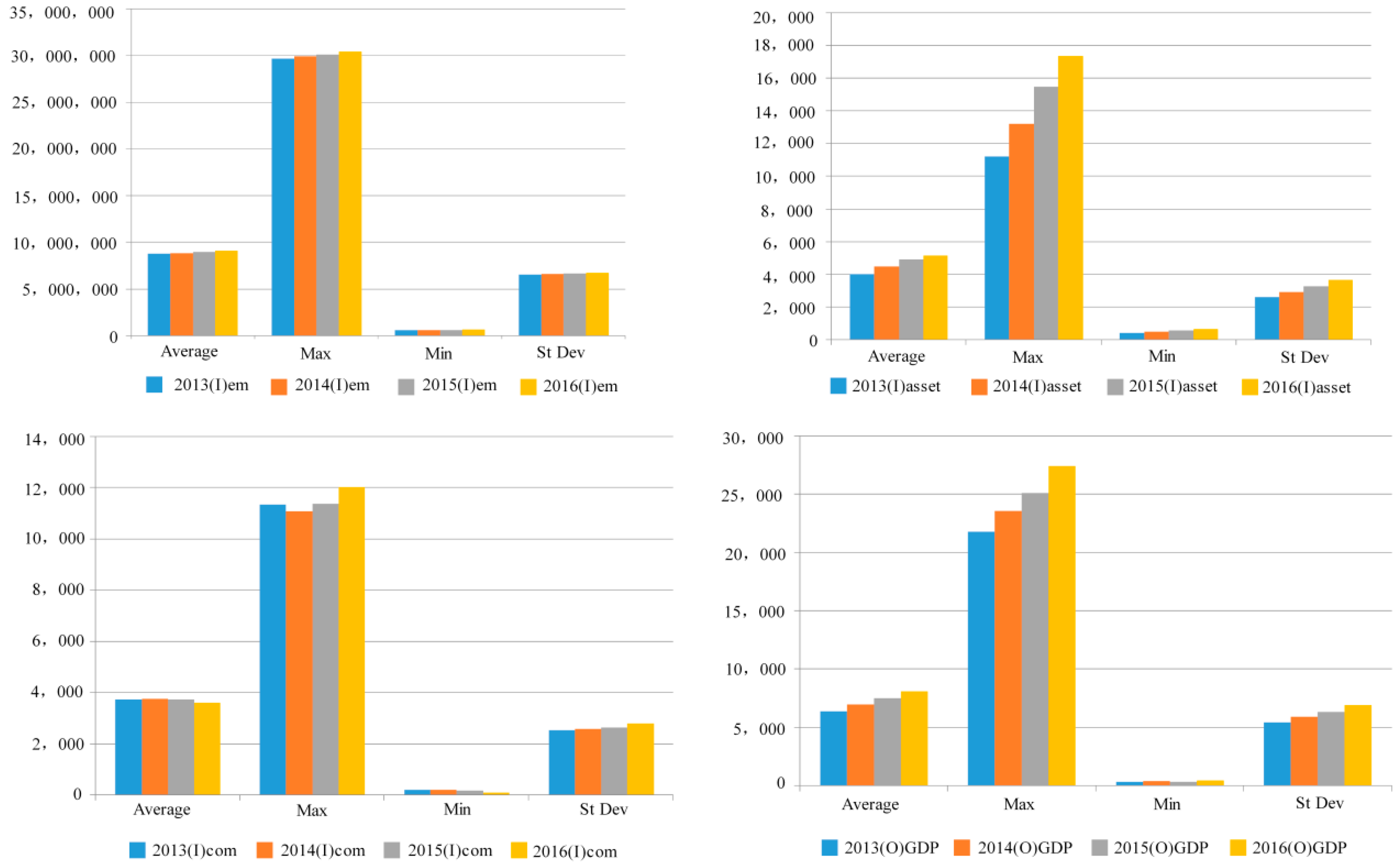
4.2. Statistical Description of the Input and Output Variables by Year

Figure 1 shows the total and growth in the input indicators for each city from 2013 to 2016. The input indicator with the largest growth was fixed assets, and the output indicator with the largest growth was GDP. The maximum value of the fixed assets rose for four years, indicating that the city asset investments increased substantially. The minimum value for the fixed assets also rose. The maximum GDP value rose, especially from 2015 to 2016. The growth in the minimum GDP fluctuated, with the value in 2015 being slightly lower than in 2014.

The growth in the maximum and minimum energy consumption in the various cities fluctuated. The consumption of traditional energy was controlled by the government, and the development of new energy was insufficient. The maximum value began to decrease in 2014 but rose again in 2015 and 2016. The minimum value continued to decline, and the average value in each city was significantly lower in 2016 than in the previous three years.

The maximum, minimum, and average value for the number of labor grew slowly, indicating that the employment population in each city was growing slowly.

Table 1. Input and output variables from 2013–2016 for high income and upper-middle income cities.

Year	City	Em	Asset	Com	GDP	CO2	AQI
2013	high income	10528121	4400	5083	9512	12481	154
	upper-middle income	7361294	3030	2400	3804	7340	146
2014	high income	10658129	5260	5136	10331	12421	94
	upper-middle income	7404954	3540	2427	4165	7388	91
2015	high income	10784014	7007	5174	11097	12264	90
	upper-middle income	7878600	3231	2255	4494	7178	81
2016	high income	10909971	6999	4141	11978	10789	81
	upper-middle income	8022387	3295	2369	4851	6714	80

shows the input-output indicators for the high-income cities and upper-middle income cities divided by the economic development level from 2013 to 2016. The average labor input in the high-income cities was significantly higher than the average labor input in the upper-middle income cities; however, the labor input in both the high income and upper-middle income cities was gradually growing.

The average fixed assets in the high-income cities was significantly higher than in the upper-middle income cities, and was continuing to rise. The average fixed assets in the upper-middle income cities grew slowly, reached a peak in 2014, and was followed by a slight decline; however, the 2016 average fixed assets were slightly higher than in 2013. The gap between the average fixed assets in the upper-middle income regions and the high-income cities expanded significantly.

The average energy consumption in the high-income cities was significantly higher than in the upper-middle income cities, was slowly rising from 2013 to 2015, but significantly declined in 2016. The average energy consumption in the upper-middle income cities was fluctuating up slowly, with average energy consumption in 2016 being slightly higher than in 2013. In 2015, the gap between the two regions was the largest; however, the gap in 2016 was the smallest.

The average GDP in both the high and middle income cities rose, but the growth in the upper-middle income cities was smaller than the significant growth in the high-income cities. In 2016, the average GDP gap between the two city types continued to expand.

There were generally higher regional average CO₂ emissions in the high-income cities than in the upper-middle income cities; however, after a peak in 2015, CO₂ emissions fell to their lowest in 2016. Carbon dioxide emissions in the upper-middle income cities fluctuated down, reached a peak in 2014, and fell to a minimum in 2016.

The differences in the average AQI index between the high-income and upper-middle income cities were very small; overall, the average AQI emissions in both sectors continued to fall significantly.

4.3. Overall Efficiency Scores in the Cities from 2013 to 2016

Table 2. Overall efficiencies in each city from 2013 to 2016.

NO	DMU	2013	2014	2015	2016
1	Beijing	1	0.99012	1	0.974027
2	Changchun	0.80295	0.793137	0.822607	0.670696
3	Changsha	0.80697	0.824076	0.834134	0.812254
4	Chengdu	0.63272	0.645835	0.662165	0.609653
5	Chongqing	0.59094	0.672697	0.644781	0.630386
6	Fuzhou	0.57638	0.588204	0.579023	0.577732
7	Guangzhou	1	1	1	1
8	Guiyang	0.38089	0.435185	0.511184	0.464409
9	Harbin	0.80323	0.78108	0.793499	0.666135
10	Haikou	0.54437	0.541118	0.491816	0.439994
11	Hangzhou	0.77885	0.801863	0.818202	0.820797
12	Hefei	0.72731	0.740621	0.736062	0.638958
13	Hohhot	0.73236	0.734324	0.739256	0.690477
14	Jinan	0.61205	0.631106	0.626497	1
15	Kunming	0.43007	0.436219	0.493753	0.480126
16	Lanzhou	0.40093	0.404111	0.415462	0.413385
17	Lhasa	0.56205	0.597495	0.510101	0.472462
18	Nanchang	0.81376	0.816825	0.783319	0.648597
19	Nanjing	0.80302	0.830223	0.866551	0.863546
20	Nanning	1	1	1	0.806337
21	Shanghai	1	1	1	1
22	Shenyang	0.67153	0.663131	0.643303	1
23	Shijiazhuang	0.38155	0.372833	0.399059	0.373983
24	Taiyuan	0.45977	0.453564	0.461354	0.454468
25	Tianjin	0.80635	0.802137	0.784291	0.779526
26	Wuhan	0.72571	0.753853	0.75465	0.752141
27	Urumqi	0.57035	0.551189	0.555959	0.490751
28	Xian	0.61933	0.638733	0.611682	0.554844
29	Xining	0.35357	0.362965	0.358296	0.371074
30	Yinchuan	0.50429	0.502102	0.501551	0.488126
31	Zhengzhou	0.88447	0.88074	0.921392	0.729051

and Figure 2 show the overall efficiencies in each city. The only two cities with overall efficiencies of 1 for all four years were Guangzhou and Shanghai; however, Beijing’s overall efficiency had a declining tendency.

There was room for improvement in the overall efficiencies in the other cities; for example, Fuzhou, Guiyang, Haikou, Kunming, Lanzhou, Lhasa, Shijiazhuang, Taiyuan, Xining, and Yinchuan all had four-year efficiencies below 0.6.

Nanning’s total efficiency dropped to around 0.8 in the last year, Zhengzhou’s four-year efficiency was 0.9 in the first three years, and dropped to 0.7 in the last year, and the other cities had efficiencies between 0.6 and 0.8.

Hangzhou and Nanjing had continuous overall efficiency increases over the four years, with the efficiencies in 2016 being slightly lower than in 2015. The overall efficiencies in Changsha, Chengdu, Guiyang, and Hohhot’s rose in the first three years and declined in the last year. More cities had declining or fluctuating overall efficiencies, and the cities with the greatest need for improvements were Shijiazhuang and Xining.

4.4. Radial DEA and Non-Radial DEA (0,1)

The results of the radial and non-radial DEA analysis for each city in this study are shown in

Table 3. 2013–2016 Epsilon Scores.

	2013	2014	2015	2016
Epsilon for EBMX	0.026	0.024	0.032	0.061
Epsilon for y	0.069	0.041	0.060	0.229

. The sample Epsilon score in this study compared the radial DEA and the non-radial DEA; the main radial analysis was close to 0 and the main non-radial analysis was close to 1. Table 2 indicates that the radial DEA model was more appropriate for this analysis.

4.5. Input and Output Indicator Efficiency

Table 4. Labor, fixed assets and energy consumption efficiencies.

NO	DMU	2013 Em	2014 Em	2015 Em	2016 Em	2013 Asset	2014 Asset	2015 Asset	2016 Asset	2013 Com	2014 Com	2015 Com	2016 Com
1	Beijing	1	0.8789	1	0.8698	1	0.956897	1	0.948593	1	0.99572	1	0.98848
2	Changchun	0.8945	0.8879	0.9071	0.8057	0.677914	0.679028	0.744306	0.609618	0.86709	0.88785	0.90711	0.80574
3	Changsha	0.9049	0.9117	0.9213	0.9324	0.49021	0.458505	0.430852	0.432527	0.65663	0.66184	0.66475	0.6529
4	Chengdu	0.777	0.786	0.7979	0.7239	0.587667	0.661442	0.708454	0.593819	0.77703	0.71246	0.7979	0.76002
5	Chongqing	0.5922	0.4446	0.4903	0.5057	0.52258	0.375987	0.359212	0.356676	0.74522	0.72643	0.78872	0.782
6	Fuzhou	0.7335	0.7431	0.737	0.7432	0.483405	0.478076	0.458925	0.444513	0.73354	0.70231	0.73697	0.7432
7	Guangzhou	1	1	1	1	1	1	1	1	1	1	1	1
8	Guiyang	0.5556	0.6099	0.6817	0.65	0.442158	0.434896	0.465152	0.366737	0.46312	0.53943	0.54857	0.59512
9	Harbin	0.894	0.8777	0.887	0.6533	0.583768	0.850411	0.857175	0.591829	0.88611	0.87771	0.88703	0.80403
10	Haikou	0.6187	0.654	0.6621	0.6203	0.709764	0.704781	0.64708	0.661342	0.70976	0.65416	0.66213	0.62017
11	Hangzhou	0.884	0.8954	0.9079	0.9255	0.631849	0.600914	0.589994	0.591099	0.73862	0.7571	0.79826	0.8017
12	Hefei	0.8484	0.855	0.8536	0.7892	0.470808	0.484956	0.473774	0.436053	0.84841	0.84963	0.85355	0.78919
13	Huhehot	0.8567	0.8556	0.8594	0.8477	0.588746	0.558191	0.650452	0.575134	0.3829	0.73635	0.72336	0.67586
14	Jinan	0.768	0.78	0.779	1	0.702048	0.672596	0.635885	1	0.51647	0.52127	0.55376	1
15	Kunming	0.6043	0.6099	0.6634	0.6542	0.467378	0.481356	0.525959	0.482591	0.52913	0.52907	0.66345	0.65417
16	Lanzhou	0.5784	0.5803	0.5948	0.6088	0.551185	0.493598	0.487664	0.460161	0.33482	0.32939	0.28058	0.30529
17	Lhasa	0.7274	0.7539	0.6825	0.6603	0.399271	0.376659	0.304786	0.300866	0.72736	0.68578	0.68249	0.66028
18	Nanchang	0.9032	0.9032	0.8844	0.7991	0.552089	0.551408	0.517058	0.43287	0.90323	0.87722	0.88442	0.79908
19	Nanjing	0.903	0.9134	0.9364	0.9526	0.483872	0.513759	0.563033	0.5782	0.64314	0.61208	0.88521	0.85895
20	Nanning	1	1	1	0.5653	1	1	1	0.538224	1	1	1	0.90062
21	Shanghai	1	1	1	1	1	1	1	1	1	1	1	1
22	Shenyang	0.8122	0.8029	0.791	1	0.361985	0.378889	0.49304	1	0.63877	0.64565	0.6389	1
23	Shijiazhuang	0.5574	0.5467	0.575	0.5601	0.458335	0.424567	0.439189	0.411768	0.38737	0.40652	0.36293	0.38334
24	Taiyuan	0.6399	0.6311	0.6417	0.6552	0.564598	0.580762	0.547815	0.570105	0.1609	0.16839	0.16698	0.20225
25	Tianjin	0.9001	0.8961	0.8873	0.901	0.451147	0.435971	0.420641	0.39076	0.69364	0.70123	0.70019	0.71149
26	Wuhan	0.8497	0.8653	0.868	0.8842	0.498609	0.477503	0.477256	0.545032	0.73546	0.724	0.76	0.74499
27	Urumqi	0.733	0.7152	0.7205	0.6724	0.687344	0.618459	0.599479	0.605195	0.59726	0.61826	0.6693	0.67244
28	Xian	0.7704	0.7832	0.7631	0.7231	0.442822	0.448231	0.549883	0.551615	0.77044	0.75798	0.76313	0.72308
29	Xining	0.5294	0.5382	0.5351	0.5539	0.446974	0.391654	0.382038	0.37516	0.22159	0.22619	0.23647	0.53344
30	Yinchuan	0.681	0.6761	0.6798	0.6916	0.425349	0.386307	0.382273	0.357123	0.36051	0.32341	0.26835	0.26067
31	Zhengzhou	0.9426	0.9399	0.9651	0.8493	0.675296	0.67411	0.667886	0.576307	0.94185	0.93836	0.96513	0.84935

and

Table 5. GDP, CO₂, and AQI efficiencies.

NO	DMU	2013 GDP	2014 GDP	2015 GDP	2016 GDP	2013 CO2	2014 CO2	2015 CO2	2016 CO2	2013 AQI	2014 AQI	2015 AQI	2016 AQI
1	Beijing	1	0.99576	1	0.98874	1	0.98723	1	0.98848	1	0.99572	1	0.98848
2	Changchun	0.91286	0.9084	0.9217	0.86009	0.89446	0.86151	0.90711	0.80574	0.6392	0.54035	0.51444	0.7879
3	Changsha	0.92007	0.92493	0.932	0.94044	0.65633	0.66214	0.66475	0.6529	0.32328	0.35681	0.35018	0.36546
4	Chengdu	0.84579	0.85014	0.8561	0.83785	0.70467	0.786	0.7979	0.76002	0.74129	0.74362	0.72416	0.76002
5	Chongqing	0.83122	0.86173	0.8515	0.84819	0.71279	0.74767	0.78872	0.782	0.74522	0.80887	0.78872	0.782
6	Fuzhou	0.82618	0.83031	0.8276	0.83034	0.69344	0.74314	0.73697	0.7432	0.66687	0.57011	0.49972	0.464
7	Guangzhou	1	1	1	1	1	1	1	1	1	1	1	1
8	Guiyang	0.76473	0.78088	0.8055	0.79411	0.5046	0.49509	0.68167	0.59512	0.18119	0.22037	0.27751	0.20594
9	Harbin	0.91254	0.90174	0.9079	0.85921	0.89399	0.87142	0.88703	0.80403	0.73713	0.80129	0.65821	0.80403
10	Haikou	0.81636	0.81438	0.7984	0.78418	0.66262	0.70478	0.66213	0.62026	0.22558	0.29087	0.25134	0.27003
11	Hangzhou	0.90585	0.91349	0.9222	0.93513	0.75228	0.74336	0.79826	0.8017	0.378	0.48974	0.41378	0.46051
12	Hefei	0.88367	0.88757	0.8867	0.85171	0.84429	0.85496	0.85355	0.78919	0.39491	0.47105	0.4615	0.5972
13	Huhehot	0.88861	0.88797	0.8902	0.88328	0.73878	0.38165	0.72336	0.67586	0.20071	0.1595	0.13775	0.13607
14	Jinan	0.84151	0.84721	0.8467	1	0.51435	0.52342	0.55376	1	0.22869	0.22691	0.18646	1
15	Kunming	0.77913	0.78086	0.7988	0.79557	0.52673	0.53148	0.66345	0.65417	0.45111	0.38618	0.45071	0.51613
16	Lanzhou	0.77127	0.77184	0.7762	0.78051	0.33008	0.33412	0.28058	0.30529	0.16444	0.12372	0.10724	0.0913
17	Lhasa	0.82356	0.83507	0.8058	0.79772	0.66087	0.75388	0.68249	0.66028	0.07486	0.05519	0.04143	0.04323
18	Nanchang	0.91892	0.91893	0.9061	0.85667	0.87871	0.90325	0.88442	0.79908	0.51376	0.51546	0.45161	0.51237
19	Nanjing	0.91877	0.92617	0.9436	0.95669	0.61022	0.6451	0.88521	0.85895	0.31616	0.69241	0.38977	0.40935
20	Nanning	1	1	1	0.9171	1	1	1	0.90062	1	1	1	0.90062
21	Shanghai	1	1	1	1	1	1	1	1	1	1	1	1
22	Shenyang	0.86346	0.85862	0.8526	1	0.65849	0.62631	0.6389	1	0.37542	0.50149	0.27621	1
23	Shijiazhuang	0.76522	0.76224	0.7703	0.76598	0.41483	0.37961	0.57496	0.38334	0.17055	0.18937	0.24116	0.1773
24	Taiyuan	0.79067	0.78771	0.7913	0.79592	0.17193	0.15759	0.16698	0.20225	0.18487	0.14374	0.12941	0.11055
25	Tianjin	0.9167	0.91399	0.908	0.91739	0.69173	0.70317	0.70019	0.71149	0.70916	0.60115	0.5781	0.55227
26	Wuhan	0.88447	0.8939	0.8956	0.90594	0.71122	0.74868	0.76	0.74499	0.32844	0.4352	0.40364	0.3624
27	Urumqi	0.82597	0.81857	0.8207	0.80209	0.62848	0.58755	0.6693	0.67244	0.15754	0.11749	0.10465	0.0939
28	Xian	0.84267	0.84876	0.8393	0.82178	0.74613	0.78318	0.76313	0.72308	0.36284	0.4332	0.40564	0.43193
29	Xining	0.75756	0.75992	0.7591	0.76423	0.22286	0.2249	0.23647	0.53344	0.09728	0.07094	0.06558	0.05917
30	Yinchuan	0.80524	0.80344	0.8048	0.80925	0.32246	0.36158	0.26835	0.26067	0.10775	0.09394	0.07349	0.06547
31	Zhengzhou	0.94853	0.94638	0.9674	0.88423	0.94262	0.93994	0.96513	0.84935	0.69037	0.59825	0.49866	0.74997

show the efficiencies for the labor, fixed assets, GDP, energy consumption, CO₂, and AQI indicators for each city from 2013 to 2016. All indicators in Guangzhou and Shanghai had efficiencies of 1 for all four years and therefore there was no need for improvements. The efficiency in Beijing from 2013–2016 reached 1 in only a few years and was worse than in Shanghai and Guangzhou. In particular, as the weather conditions in Shanghai and Guangzhou are better than in Beijing, the spread of the air pollutants was better.

The labor efficiencies were higher than the fixed assets and energy consumption efficiencies. Cities with labor efficiencies below 0.6 for all four years included Chongqing, Lanzhou, Shijiazhuang, and Xining, all of which are in the central and western parts of China where both economic and social development is still relatively low and labor inefficiencies are generally related to labor productivity. Labor efficiency increased over time in most cities; however, in Beijing, Lhasa, Harbin, Nanchang, Urumqi, and Xian, it declined or fluctuated over the four years, and in Changchun, Chengdu, Guiyang, Hefei, and Zhengzhou it dropped significantly in 2016.

The fixed assets efficiencies in each city were lower than the labor and energy consumption efficiencies, and most cities had generally lower efficiencies for all four years, except for Guangzhou and Shanghai with fixed assets efficiencies of 1 for all four years. However, improvements were needed in all other regions. Beijing, Changchun, Chengdu, Harbin, Jinan, Nanning, Shenyang, Urumqi, and Zhengzhou had annual efficiencies above or close to 0.6, Beijing’s fixed assets efficiency was 1 in 2013 and 2015, but only 0.95 in 2014 and 2016, and in other cities, the fixed assets efficiency was generally below 0.7. Seventeen cities had fixed assets efficiencies of less than 0.6 for four years, with the lowest being in Lhasa at only 0.4 in 2013, after which it continued to drop to close to 0.3. Only a few cities had rising fixed assets efficiencies such as Nanjing, Shenyang, Wuhan, and Xian. The most significant fixed assets efficiency rise was in Shenyang, which rose from around 0.3 in 2013 to 1 in 2016; Jinan’s rise was also large, from less than 0.6 in 2013 to 1 in 2016. More cities had declining fixed assets efficiencies; for example, Nanning’s dropped significantly in 2016 to around 0.54, and Chongqing’s also fell from around 0.5 in 2013 to below 0.4 in 2014, and then to nearly 0.3 in 2016.

The differences between the energy consumption efficiencies were very large. Guangzhou and Shanghai had efficiencies of 1, Beijing’s dropped slightly to 0.98 in 2014 and 2016, and Nanning’s efficiency was 1 in 2013 and 2015 but dropped to 0.9 in the final year. Five cities—Changchun, Harbin, Hebei, Nanchang, and Zhengzhou—had energy consumption efficiencies above 0.8 in all four years, but Guiyang, Lanzhou, Shijiazhuang, Taiyuan, and Yinchuan had efficiencies below 0.6 in all four years. The city with the lowest energy consumption efficiency was Taiyuan, which had its highest efficiency of only 0.2 in 2016. Taiyuan’s main industries are focused on the coal and the petrochemical industries and therefore it has large carbon dioxide emissions and air pollutant emissions. While Lanzhou’s efficiency was slightly better than Taiyuan, its best efficiency was only around 0.3 in 2013, after which it fell.

Chongqing, Fuzhou, Guiyang, Hangzhou, Huhehot, Jinan, Kunming, Nanjing, Shenyang, Taiyuan, Tianjin, Wuhan, Urumqi, and Xining had increasing energy consumption efficiencies. The city with the largest increase was Jinan, which rose from an efficiency of around 0.5 in 2013 to 1 in 2016. Shenyang’s efficiency was slightly higher than 0.6 in 2013 and rose to 1, and Xining’s rose slightly from 0.2 in 2013 to slightly above 0.5 in 2016.

Cities with declining energy consumption efficiencies for all years were Beijing, Changchun, Changsha, Chengdu, Harbin, Hefei, Lanzhou, Lhasa, Nanchang, Nanning, Shijiazhuang, Xian, Yinchuan, and Zhengzhou, most of which experienced slow declines. The cities with relatively large energy consumption efficiency declines were Harbin, Nanchang, and Yinchuan.

The GDP efficiencies in each city were generally high, with most cities having efficiencies above 0.7. The efficiencies in Beijing, Guangzhou, Shenyang, and Nanning were 1 for the first three years but fell to around 0.9 in 2016. Cities with relatively poor GDP efficiencies were Guiyang, Kunming, Lanzhou, Shijiazhuang, Taiyuan, and Xining, all of which were below 0.8.

Cities with rising GDP efficiencies were Changsha, Chongqing, Guiyang, Hangzhou, Jinan, Kunming, Lanzhou, Nanjing, Shenyang, Taiyuan, Tianjin, Wuhan, Xining, and Yinchuan, with Jinan having the largest rise from 0.8 in 2012 to 1 in 2016. Shenyang’s GDP efficiency was close to 0.85 in 2013, declined slightly in 2014 and 2015, and rose to 1 in 2016. While the GDP efficiency in the other cities declined, the decline was small.

As Figure 3 shows, Guangzhou and Shanghai had CO₂ efficiencies of 1 for 4 years, Beijing’s fell slightly to 0.98 in 2014 and 2016, and Nanning’s fell to around 0.9 in 2016. Nanning’s efficiency for the first three years was 1, but fell to around 0.9 in the last year. Other cities with efficiencies above 0.9 for all four years were Changchun, Harbin, Hefei, Nanchang, and Zhengzhou.

The city with the worst CO₂ efficiency was Taiyuan, with efficiencies in all years being below 0.2, followed by Lanzhou, where the highest efficiency was around 0.33 in 2014. Xining’s efficiency for 2016 was only slightly above 0.5, but was below 0.3 in the other years. The other cities had CO₂ efficiencies between 0.5 and 0.8. Generally, the cities with the greatest need for improvements were cities in the relatively less developed central and western regions.

Cites in which the CO₂ efficiencies were declining were Changchun, Changsha, Harbin, Guiyang, Haikou, Huhehot, Lanzhou, Lhasa, Nanchang, Nanning, Shijiazhuang, Xian, and Zhengzhou, with the largest declines being in Harbin and Nanchang; however, the magnitude was not large.

Except for Guangzhou and Shanghai, the CO₂ efficiencies in the other 16 cities increased. The city with the largest increase was Jinan, rising from 0.5 in 2013 to 1 in 2016, followed by Shenyang, which rose slightly from 0.6 in 2013 to 1 in 2016.

Lanzhou, Taiyuan, and Yinchuan had CO₂ efficiencies of less than 0.4 over the four years; however, Lanzhou and Taiyuan’s increased slightly in the last two years, while Yinchuan’s had a significant decline. Xining’s efficiency in the first three years was around 0.2, but by 2016, it had risen significantly to above 0.5. Changsha, Chengdu, Chongqing, Fuzhou, Haikou, Hangzhou, Lhasa, Tianjin, Wuhan, Urumqi and Xian had efficiencies between 0.8 and 0.6, Hohhot’s efficiency fell below 0.4 in 2014 and was between 0.6 and 0.8 in the other years, and Shenyang’s rose significantly to 1 in the last year. Therefore, the CO₂ efficiencies increased in half the cities, but declined in the other half. Chengdu, Chongqing, Fuzhou, Guiyang, Hangzhou, Jinan, Kunming, Nanjing, Shenyang, Taiyuan, Tianjin, Urumqi, and Xining had increased efficiencies, indicating that the need for improvements was shrinking, and Changchun, Changsha, Harbin, Haikou, Hebei, Lhasa, Nanchang, Nanning, Xian, Yinchuan, and Zhengzhou had declining efficiencies, indicating that the need for improvements was increasing.

The AQI efficiencies in each city were significantly lower than the CO₂ efficiencies. Of the 31 cities, only Guangzhou and Shanghai had AQI efficiencies of 1, Beijing’s declined slightly in 2014 and 2016, and Nanning attained 1 in the first three years but dropped to 0.9 in the final year. More cities had very low AQI efficiencies, with Changsha, Guiyang, Haikou, Hohhot, Lanzhou, Lhasa, Taiyuan, Urumqi, Xining, and Yinchuan all having AQI efficiencies below 0.4 for all four years, and with Hohhot, Lanzhou, Lhasa, Taiyuan, Urumqi, Xining, and Yinchuan all being lower than 0.2. Changchun, Fuzhou, Hangzhou, Hebei, Kunming, Nanchang, and Tianjin had efficiencies between 0.4 and 0.6 for three years, and Chengdu, Chongqing, Harbin, and Zhengzhou had efficiencies between 0.6 and 0.8.

Twelve cities had continuous efficiency declines; Beijing, Fuzhou, Huhehot, Lanzhou, Lhasa, Nanchang, Nanning, Taiyuan, Tianjin, Urumqi, Xining, and Yinchuan. Fuzhou, the city with the largest decline, fell from around 0.7 in 2013 to less than 0.5 in 2016.

Except for Guangzhou and Shanghai, the AQI efficiencies in 17 cities increased. The city with the largest increase was Jinan, which rose from 0.2 in 2013 to 1 in 2016, followed by Shenyang, which was close to but below 0.4 in 2013 but rose to 1 in 2016. In the other cities, there was a small increase.

Chengdu (slightly down in 2015, rose to above 0.7 in 2016), Harbin (significantly dropped to 0.7 in 2015, and rebounded to 0.8 in 2016), Jinan (significantly rose to 1 in 2016), Kunming (also slightly lower than 2013 in 2014, and then continued to rise), Nanjing, Nanchang, Shenyang, Xian, and Zhengzhou had generally rising efficiencies. Overall, the AQI efficiencies in seven cities were still falling and the need for improvement was increasing.

There were large differences in the CO₂ emissions and air pollution emissions efficiencies in the cities.

Table 6. CO₂ and AQI comparisons and policy suggestions.

NO	DMU
1	Beijing	The CO2 efficiency was slightly lower than the AQI efficiency, CO2 emissions and air pollutant emissions need to be and comprehensively treated.
2	Changchun	The CO2 efficiency was better than the AQI efficiency and fluctuated down. The AQI efficiency had a greater need for improvement, but rose and made significant progress.
3	Changsha	The CO2 efficiency was better than the AQI efficiency, the CO2 efficiency was slightly higher than 0.6, and the AQI efficiencies were all lower than 0.4; therefore, the AQI should be treated.
4	Chengdu	The CO2 and AQI efficiencies were basically the same. The AQI was slightly lower than the CO2, so there should be an increased focus on AQI monitoring and governance.
5	Chongqing	As the CO2 and AQI efficiencies were basically the same, both the AQI and CO2 need attention.
6	Fuzhou	The AQI efficiency was lower than the CO2, and the AQI efficiency continued to decline, requiring a focus on AQI and then joint governance
7	Guangzhou	Optimal.
8	Guiyang	The AQI efficiency was lower than the CO2, and AQI efficiency continued to decline, requiring a focus on AQI and then joint governance
9	Harbin	The AQI efficiency was slightly lower than the CO2; therefore, priority should be given to AQI.
10	Haikou	The AQI efficiency was slightly lower than the CO2; therefore, priority should be given to AQI.
11	Hangzhou	The AQI efficiency was significantly lower than the CO2; therefore, priority should be given to the AQI and some measures taken to reduce CO2.
12	Hefei	The AQI efficiency was significantly lower than the CO2; therefore, priority should be given to the AQI and some measures taken to reduce CO2.
13	Huhehot	The AQI efficiency was significantly lower than the CO2; therefore, priority should be given to the AQI and some measure taken to reduce CO2.
14	Jinan	Comprehensively manage both AQI and CO2, but pay more attention to the AQI
15	Kunming	The AQI efficiency was slightly lower than the CO2; therefore, priority should be given to AQI.
16	Lanzhou	Neither of the two indicators were efficient, but the AQI was less efficient; therefore, priority should be given to AQI and then focus placed on comprehensive governance.
17	Lhasa	The AQI efficiency was slightly lower than the CO2,
18	Nanchang	The AQI efficiency was significantly lower than the CO2; therefore, priority should be given to the AQI and some measures taken to reduce CO2.
19	Nanjing	The AQI efficiency was significantly lower than the CO2; therefore, priority should be given to the AQI and some measures taken to reduce CO2.
20	Nanning	Both indicators were good, with less than 1 in 2016. Co-governance should be strengthened to maintain effective carbon dioxide emissions and air pollution control
21	Shanghai	Both achieved the best; strengthen comprehensive management and monitoring, lead new technology analysis and governance model analysis.
22	Shenyang	Both indicators reached 1. The AQI efficiency was lower than the CO2 in 2016; therefore, comprehensive management needs to be strengthened.
23	Shijiazhuang	The AQI efficiency was slightly lower than the CO2; therefore, priority should be given to AQI.
24	Taiyuan	Both indicators had a lot of room for improvement, CO2 emission efficiency had not changed much, AQI has continued to decline, and joint governance needs to be strengthened with AQI as the priority.
25	Tianjin	The AQI efficiency was slightly lower than the CO2; therefore, priority should be given to AQI.
26	Wuhan	The AQI efficiency was significantly lower than the CO2; therefore, priority should be given to the AQI and some measures taken to reduce CO2.
27	Urumqi	The AQI efficiency was significantly lower than the CO2; therefore, priority should be given to the AQI, and some measures taken to reduce CO2.
28	Xian	The AQI efficiency was significantly lower than the CO2; therefore, priority should be given to the AQI and some measures taken to reduce CO2.
29	Xining	The AQI efficiency was significantly lower than the CO2; therefore, priority should be given to the AQI and some measures taken to reduce CO2.
30	Yinchuan	The AQI efficiency was significantly lower than the CO2; therefore, priority should be given to the AQI, and some measures taken to reduce CO2.
31	Zhengzhou	The AQI efficiency was significantly lower than the CO2; therefore, priority should be given to the AQI and some measures taken to reduce CO2.

compares the CO₂ and AQI efficiency scores in the cities from 2013 to 2016 and suggests mitigation policies.

4.6. Technology Gap Based on the Meta-Frontier

Table 7. Metafrontier efficiency score.

NO	City	Cluster	Score_Metafrontier				Score_GroupFrontier
			2013	2014	2015	2016	2013	2014	2015	2016
1	Beijing	1	1	0.99012	1	0.974027	1	1	1	0.97556
2	Changchun	2	0.802947	0.793137	0.822607	0.670696	1	1	1	1
3	Changsha	1	0.806968	0.824076	0.834134	0.812254	0.806968	0.8182	0.839665	0.852228
4	Chengdu	2	0.632719	0.645835	0.662165	0.609653	1	1	1	1
5	Chongqing	2	0.590943	0.672697	0.644781	0.630386	1	1	1	1
6	Fuzhou	1	0.576382	0.588204	0.579023	0.577732	0.581444	0.59568	0.582666	0.586273
7	Guangzhou	1	1	1	1	1	1	1	1	1
8	Guiyang	2	0.380893	0.435185	0.511184	0.464409	0.682644	0.779521	0.83947	0.835986
9	Harbin	2	0.803228	0.78108	0.793499	0.666135	0.940469	1	0.997395	0.988392
10	Haikou	2	0.54437	0.541118	0.491816	0.439994	0.814904	0.774701	0.699059	0.717586
11	Hangzhou	1	0.778851	0.801863	0.818202	0.820797	0.778851	0.797969	0.821858	0.847579
12	Hefei	2	0.727305	0.740621	0.736062	0.638958	0.923535	0.950402	1	1
13	Huhehot	1	0.73236	0.734324	0.739256	0.690477	0.73236	0.727379	0.743276	0.720714
14	Jinan	1	0.612053	0.631106	0.626497	1	0.612053	0.627158	0.629732	1
15	Kunming	2	0.430069	0.436219	0.493753	0.480126	0.831061	0.793866	0.803154	0.820987
16	Lanzhou	2	0.400925	0.404111	0.415462	0.413385	0.766746	0.732258	0.748767	0.774385
17	Lhasa	2	0.562054	0.597495	0.510101	0.472462	0.750872	0.824862	0.703003	0.784896
18	Nanchang	1	0.813763	0.816825	0.783319	0.648597	0.883554	0.899875	0.823818	0.65907
19	Nanjing	1	0.803019	0.830223	0.866551	0.863546	0.803019	0.826376	0.870422	0.894004
20	Nanning	2	1	1	1	0.806337	1	1	1	1
21	Shanghai	1	1	1	1	1	1	1	1	1
22	Shenyang	1	0.67153	0.663131	0.643303	1	0.67153	0.660407	0.646341	1
23	Shijiazhuang	2	0.381554	0.372833	0.399059	0.373983	0.681266	0.673301	0.682719	0.691854
24	Taiyuan	2	0.45977	0.453564	0.461354	0.454468	0.834646	0.881193	0.852663	0.94728
25	Tianjin	1	0.806349	0.802137	0.784291	0.779526	0.806349	0.798527	0.78787	0.805359
26	Wuhan	1	0.725711	0.753853	0.75465	0.752141	0.725711	0.75029	0.758022	0.778709
27	Urumqi	2	0.570352	0.551189	0.555959	0.490751	1	1	1	1
28	Xian	2	0.619327	0.638733	0.611682	0.554844	0.857289	0.893444	0.902854	0.901761
29	Xining	2	0.353568	0.362965	0.358296	0.371074	0.61316	0.64622	0.641291	0.670943
30	Yinchuan	2	0.504285	0.502102	0.501551	0.488126	0.874129	0.888917	0.898318	0.895715
31	Zhengzhou	1	0.884466	0.88074	0.921392	0.729051	1	1	1	0.734394

shows the efficiency in each city within each region and the efficiency within all 31 cities. As can be seen, most cities had higher regional comparative efficiencies than when compared to the whole country; that is, the efficiency in each city in each region compared to all 31 cities was slightly higher.

The group efficiencies for each city were higher than the overall country. In regional efficiencies, Changchun, Chengdu, Chongqing, Guangzhou, Nanning, Shanghai, and Urumqi had group efficiencies of 1, and Beijing and Zhengzhou had 1 in the first 3 years, but 0.98 and 0.73 in 2016.

There were also differences in the efficiencies of cities in the region and efficiencies across the country. Changsha’s regional efficiency score continued to rise; however, while the country-wide efficiencies showed volatile increases, this was less than the regional increases. For example, Guiyang’s regional efficiency rose sharply, but in the country-wide efficiency assessment, it only slightly increased, and regionally, Harbin has fluctuating efficiencies above 0.98, but the country-wide efficiency comparison showed a decline, and by 2016 was only around 0.67.

Most cities with high regional efficiency had low national efficiency. Haikou scored high in regional efficiency, but its national efficiency continued to fall from 0.54 in 2013 to around 0.44 in 2016. Hefei’s regional efficiency was higher than 0.9 and was 1 in the last two years; however, its national efficiency was only about 0.7, and by 2016 it was only about 0.64. This was also seen in Kunming.

Except for Guangzhou and Shanghai, the efficiencies in the other five cities were lower in the all-cities comparison; Changchun was about 0.8, Chengdu was around 0.6, Chongqing was below 0.7, and Urumqi was below 0.6; even though these cities had high efficiency scores in their own group. However, because of the differences in the regional economic development stages, the efficiencies in the different city groups were quite different. Compared with the other cities in the country, the efficiencies in the above cities were low.

Guangzhou and Shanghai, as well as Beijing and Nanning all achieved 1 in several years. Overall, however, the efficiencies over the four years in most cities was below 0.8, with Lanzhou, Shijiazhuang, and Xining having efficiencies of less than 0.4.

Table 8. Technology gap ratio based on metafrontier.

NO	DMU	Cluster	2013	2014	2015	2016
1	Beijing	1	1	0.99012	1	0.998429
2	Changchun	2	0.802947	0.793137	0.822607	0.670696
3	Changsha	1	1	1.007182	0.993413	0.953095
4	Chengdu	2	0.632719	0.645835	0.662165	0.609653
5	Chongqing	2	0.590943	0.672697	0.644781	0.630386
6	Fuzhou	1	0.991294	0.98745	0.993748	0.985432
7	Guangzhou	1	1	1	1	1
8	Guiyang	2	0.557967	0.558272	0.608937	0.555522
9	Harbin	2	0.854072	0.78108	0.795571	0.673958
10	Haikou	2	0.668017	0.698486	0.70354	0.613159
11	Hangzhou	1	1	1	0.995552	0.968402
12	Hefei	2	0.787523	0.779271	0.736062	0.638958
13	Hohhot	1	1	1	0.994592	0.958046
14	Jinan	1	1	1	0.994863	1
15	Kunming	2	0.517494	0.549487	0.614768	0.584816
16	Lanzhou	2	0.522892	0.55187	0.554862	0.533824
17	Lhasa	2	0.748535	0.724358	0.725603	0.601942
18	Nanchang	1	0.921011	0.907709	0.95084	0.984109
19	Nanjing	1	1	1	0.995553	0.965931
20	Nanning	2	1	1	1	0.806337
21	Shanghai	1	1	1	1	1
22	Shenyang	1	1	1	0.9953	1
23	Shijiazhuang	2	0.560066	0.553739	0.584514	0.540552
24	Taiyuan	2	0.550856	0.514716	0.541074	0.479761
25	Tianjin	1	1	1	0.995457	0.967924
26	Wuhan	1	1	1	0.995552	0.965882
27	Urumqi	2	0.570352	0.551189	0.555959	0.490751
28	Xian	2	0.722425	0.714911	0.677498	0.615289
29	Xining	2	0.576633	0.561674	0.55871	0.553063
30	Yinchuan	2	0.5769	0.564847	0.558322	0.544957
31	Zhengzhou	1	0.884466	0.88074	0.921392	0.992725

and Figure 4 show the technology gaps in each city; the higher the technology gap ratio of the city, the better the technology. Beijing, Changsha, Fuzhou, Guangzhou, Hangzhou, Hohhot, Jinan, Nanjing, Shanghai, Shenyang, Tianjin, and Wuhan had high technology gap ratios (above 0.95 and close to 1), Guiyang, Kunming, Lanzhou, Shijiazhuang, Taiyuan, Urumqi, Xining, and Yinchuan had technology gap ratios below 0.6, all of which except for Shijiazhuang, are located in the central and western regions of China and have significantly lower economic and social development than the developed cities in the coastal areas.

Changchun, Chengdu, Chongqing, Haikou, Hefei, Lhasa, Xian. Haikou and Lhasa had technology gap ratios between 0.6 and 0.8 and had significantly better air pollution treatments due to their specific geographical locations and meteorological conditions, and had their main economic growth coming from tourism, rather than from high-emitting, high-polluting industries. Chengdu, Chongqing, and Xian were among the fastest-growing cities in the western region, and were also ahead of the other cities in the west in technology and innovation.

From 2013 to 2016, the technology gap in Changsha, Hangzhou, Harbin, Hohhot, Hefei, Lhasa, Nanjing, Nanning, Tianjin, Wuhan, Urumqi, Xian, Xining, and Yinchuan was declining; however, the technology gap in Chengdu, Haikou, Kunming, Lanzhou, Nanchang, and Zhengzhou was widening, with Zhengzhou rising the most significantly to nearly 1. The technology gap in other cities in 2016 dropped significantly; for example, in Changchun, the technology gap dropped from 0.82 in 2015 to 0.67 in 2016.

Table 9. Technology Gap Ratio for high-income cities and upper-middle income cities.

City	2013 Technology Gap Ratio	2014 Technology Gap Ratio	2015 Technology Gap Ratio	2016 Technology Gap Ratio
high income	0.985484	0.9838	0.98759	0.981427
upper-middle income	0.661197	0.659739	0.667351	0.596684

shows the Technology Gap Ratios for the high-income and upper-middle income cities, from which it can be seen that the average Technology Gap Ratios in the high-income cities was significantly higher, with all being 1, than in the upper-middle income cities. The average Technology Gap Ratio for the upper-middle income cities did not exceed 0.7, and there were significant regional differences.

The changes in the average Technology Gap Ratios in the high-income cities was not obvious, with only a small rise and then a fall. The fluctuations in the average Technology Gap Ratios in the upper-middle income cities was quite obvious, however, and by 2016, it was down 0.7 compared to 2013.

Overall, the high-income cities had a large lead compared to the upper-middle income cities, and therefore, more governance is need in the upper-middle income cities.

5. Conclusions and Policy Recommendations

This research used a metafrontier EBM and divided 31 Chinese cities into high-income and upper-middle income cities to compare city efficiencies, with labor, fixed assets, energy consumption as the inputs, GDP as the desirable output, and CO₂ and AQI as the undesirable outputs, the results from which are as follows:

• The input and output inefficiencies were mainly affected by radial inefficiency, with only a few cities being affected by non-radial inefficiencies.
• The average labor input, average fixed assets input, average energy consumption, average GDP and average CO₂ emissions efficiencies in the high-income cities were significantly greater than the efficiencies in the upper-middle income cities. The regional gap between the average fixed assets input and the average GDP output was found to be widening; however, the regional average energy consumption input differences were the lowest in 2016 and the differences in the average labor input and AQI emissions efficiencies did not change significantly.
• The regional efficiencies in the upper-middle income cities were generally higher than their national efficiencies. Of the 31 cities, only Guangzhou and Shanghai had input and output efficiencies of 1 for all four years in both the regional and all city comparisons.
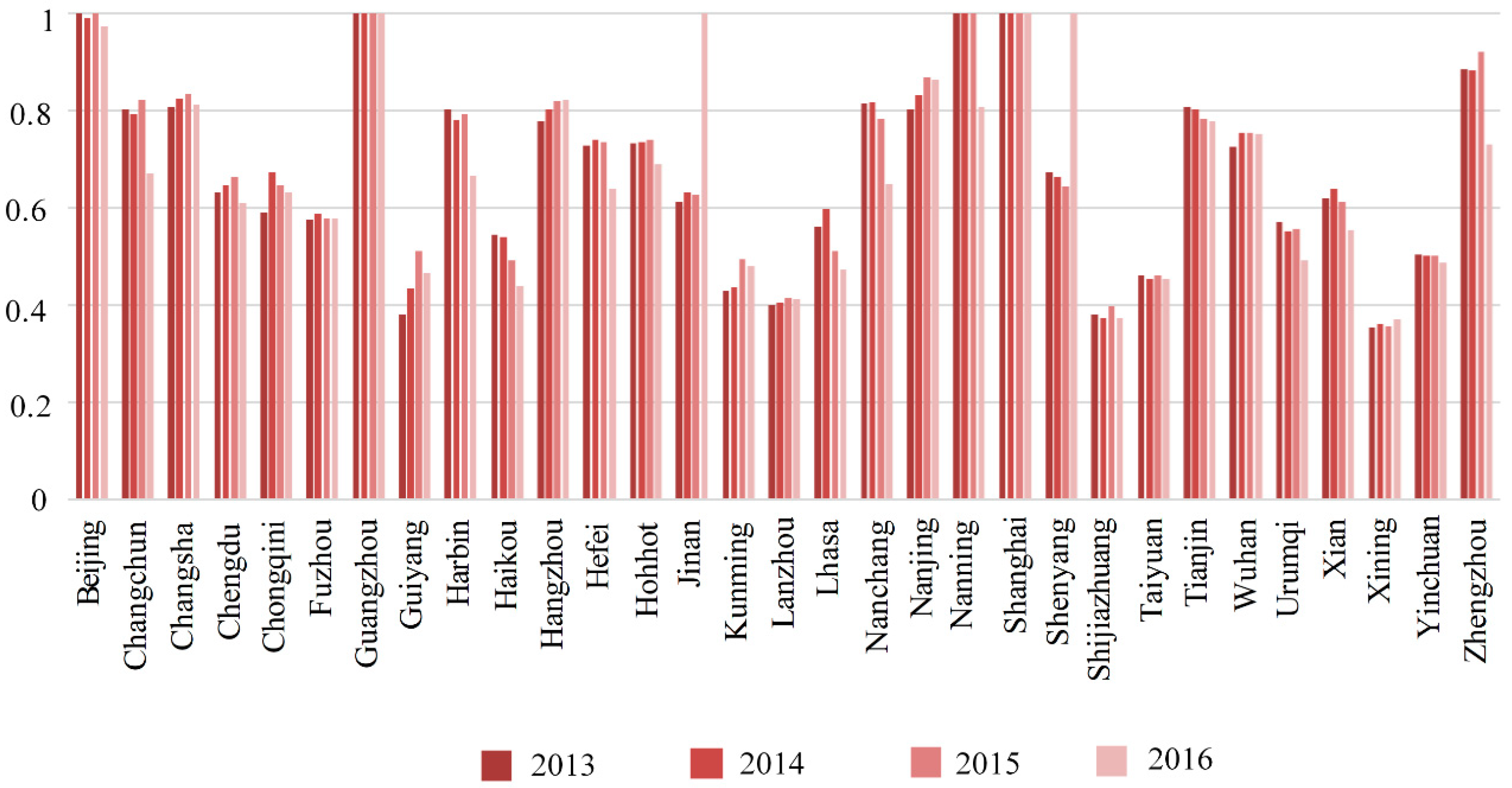
• The labor efficiencies in most cities were higher than the fixed assets and energy consumption efficiencies. The upper-middle income cities of Chongqing, Lanzhou, Shijiazhuang, Xining had labor efficiencies below 0.6; however, while the labor efficiencies increased in most cities, there were 11 cities with declining labor efficiencies over all four years, with the upper-middle income cities of Changchun, Chengdu, Guiyang, Hefei, and Zhengzhou declining the most significantly.
• The fixed assets input efficiencies were lower than the labor and energy consumption input efficiencies, and there were 17 cities with fixed asset indicators below 0.6 in all four years. Lhasa had lowest fixed asset efficiency; Nanjing, Shenyang, Wuhan, and Xian had increasing fixed asset efficiencies; and more upper-middle income cities had declining fixed-assets efficiencies than the high-income cities.
• The energy consumption efficiencies in each city were very different. Guangzhou and Shanghai had efficiencies of 1, and Beijing and Nanning’s were higher than 0.9. However, in most other cities, there was a significant need for improvements; Guiyang, Lanzhou, Shijiazhuang, Taiyuan, Yinchuan had efficiencies of less than 0.6 for four years, and Taiyuan and Lanzhou had the lowest energy consumption efficiencies. Chongqing, Fuzhou, Guiyang, Hangzhou, Huhehot, Jinan, Kunming, Nanjing, Shenyang, Taiyuan, Tianjin, Wuhan, Urumqi, and Xining, however, had increasing efficiencies, while Beijing, Changchun, Changsha, Chengdu, Harbin, Hefei, Lanzhou, Lhasa, Nanchang, Nanning, Shijiazhuang, Xian, Yinchuan, Zhengzhou had declining efficiencies, all of which were upper-middle income cities, except for Beijing.
• The GDP efficiencies were generally high, with 11 cities experiencing GDP efficiency increases; however, seven cities had declining efficiencies. Cities with relatively poor efficiencies were Guiyang, Kunming, Lanzhou, Shijiazhuang, Taiyuan and Xining. Changsha, Chongqing, Guiyang, Hangzhou, Jinan, Kunming, Lanzhou, Nanjing, Shenyang, Taiyuan, Tianjin, Wuhan, Xining, Yinchua had increasing efficiencies for all four years, while the other cities had declining efficiencies.
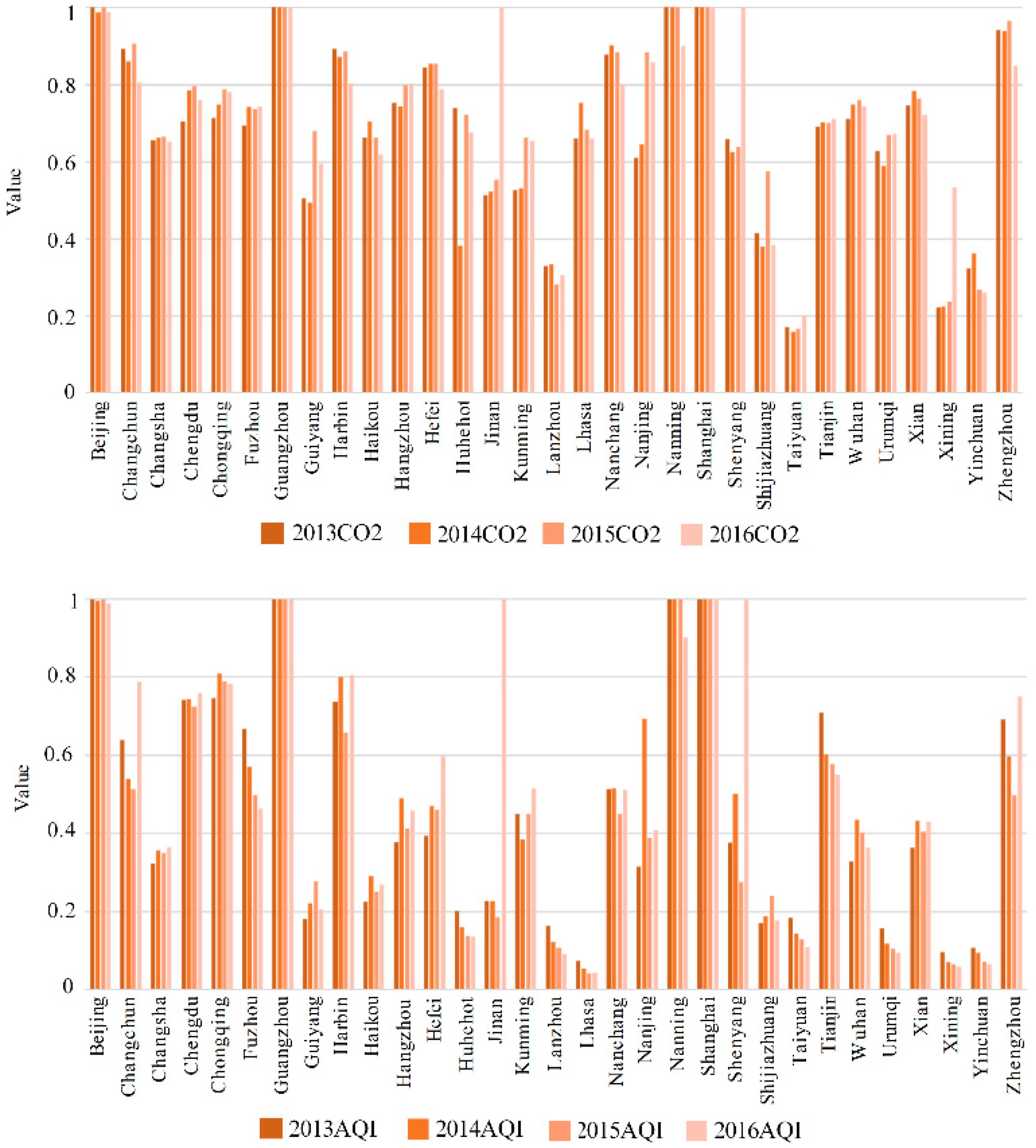
• Guangzhou and Shanghai’s CO₂ efficiencies were 1 for all four years, and Beijing Changchun, Harbin, Hefei, Nanchang, Zhengzhou had CO₂ efficiencies over 0.9; however, the other cities were performing poorly. Taiyuan, Lanzhou and Yinchuan performed the worst, primarily because these cities are all dependent on the coal industry. There were decreasing CO₂ efficiencies in Changchun, Changsha, Harbin, Guiyang, Haikou, Huhehot, Lanzhou, Lhasa, Nanchang, Nanning, Shijiazhuang, Xian, and Zhengzhou, with the largest declines being in Harbin and Nanchang. The other 16 cities had increasing CO₂ efficiencies.
• The AQI efficiencies were generally lower than the CO₂ efficiencies. Guangzhou and Shanghai had AQI efficiencies of 1, and Beijing and Nanning’s were slightly better; however, the other cities had significant room for improvement. The AQI efficiencies in 10 upper-middle income cities—Changsha, Guiyang, Haikou, Huhehot, Lanzhou, Lhasa, Taiyuan, Urumqi, Xining, and Yinchuan—were below 0.4, seven cities had efficiencies between 0.4 and 0.6, and 4 cities had efficiencies between 0.6 and 0.8. The AQI efficiencies in nine upper-middle income and three high-income cities declined—Beijing, Fuzhou, Huhehot, Lanzhou, Lhasa, Nanchang, Nanning, Taiyuan, Tianjin, Urumqi, Xining, and Yinchuan.
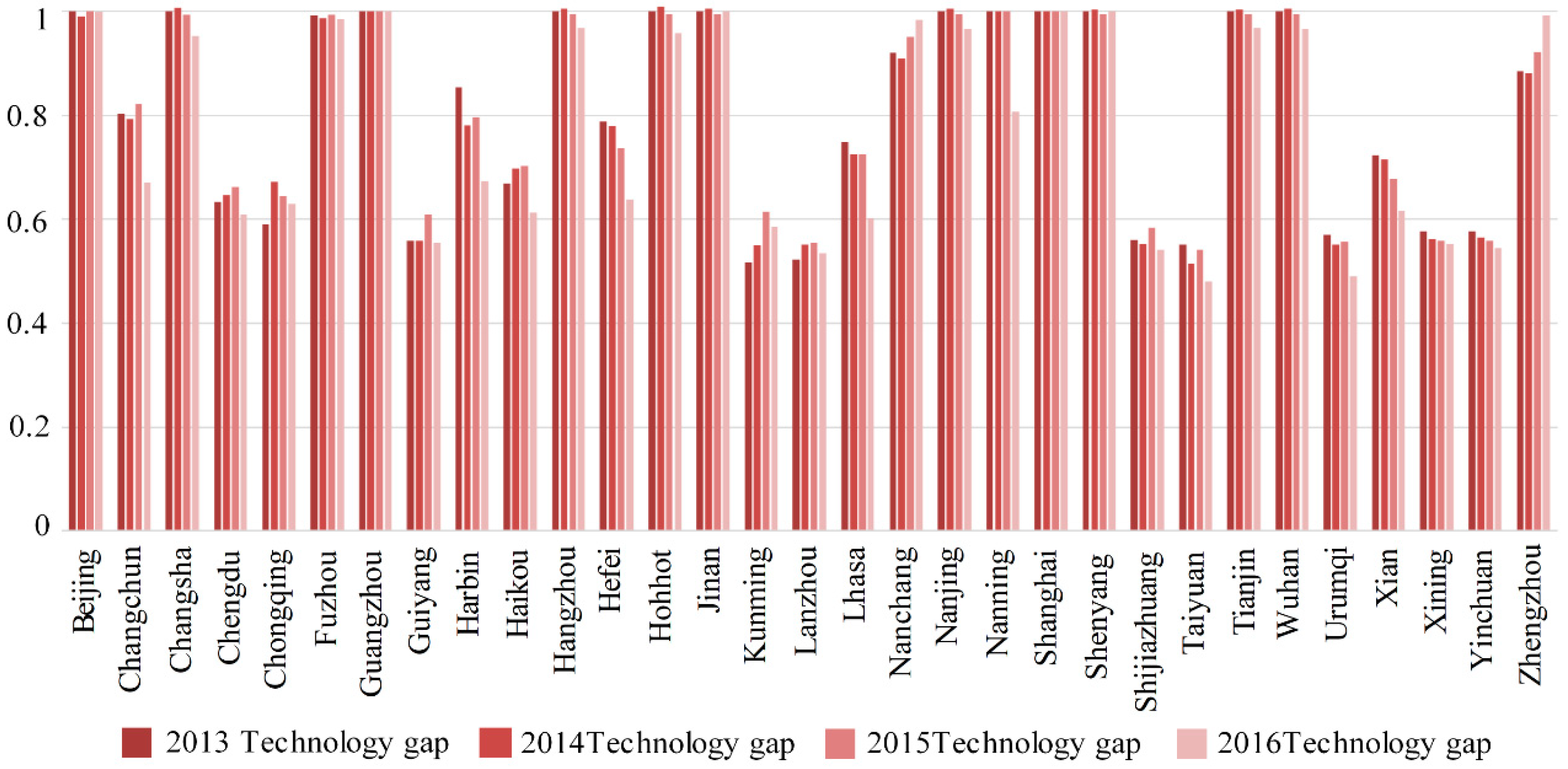
• The technology gap between the cities was large. The technology gap ratio in 12 cities was high (higher than 0.95) and close to 1; in eight cities, it was below 0.6 and in seven cities, it was between 0.6 and 0.8. The technology gap was falling in 14 cities and rising in six cities. The average Technology Gap Ratio in the high-income cities was significantly higher than in the upper-middle income cities and there were large differences between the cities. There was a significantly downward fluctuation in the average Technology Gap Ratios of the upper-middle income cities.

Based on the above research conclusions, it was obvious that the high-income cities were more efficient than the upper-middle income cities. Based on these results, the following policy recommendations are given.

• Rational allocation and effective use of resources: There is still significant room for improvement in production, human resources, capital assets, and energy consumption investments in many cities. The use of resources in the less-developed areas of central and western China was found to be less effective; therefore, cross-regional resource flows and effective resource allocations within the region should be promoted.
• Economic growth needs to consider sustainable economic and environmental development when developing CO₂ and AQI governance policies. In the past five years, the central government has introduced many regulatory air pollution control measures. Although some achievements have been made, there are great challenges. There is still a lot of room for improvement in the AQI in most cities, and although CO₂ emissions efficiencies were found to be somewhat better than the AQI efficiencies, regulations and controls still need to be strengthened; therefore, it is important to develop comprehensive CO₂ and AQI emissions control regulations.
• Problems in each city: As there are significant regional differences in Chinese cities, the CO₂ and AQI efficiencies varied widely. As most coastal high-income cities are now less dependent on petrochemical and coal energy, the industrial and economic developments result in less air pollution; however, because of the high population densities, there remain some carbon dioxide emissions and other pollution problems. Therefore, high-income cities need to focus on strengthening their carbon dioxide emissions control, and cities such as Haikou, which has good meteorological conditions, need to adjust their industrial structure to deal with air pollution.
• Most low-income cities located in the west and middle west of China require industrial structural adjustment to reduce their dependence on coal and petrol energy. Therefore, carbon emissions trading markets and AQI emissions trading markets should be established to reduce emissions.
• High-income cities should learn from Western developed countries and combine their own resource endowments and characteristics to strengthen comprehensive governance and promote environmentally friendly enterprises. High-income cities should also provide advanced experience to other relatively backward cities.

There is still a need for improvements in carbon emissions and air pollution efficiencies in most cities; however, local geographical conditions, meteorological conditions, economic development stages, and technical levels need to be considered when developing carbon emissions and air pollution treatments in cities.

• The carbon emissions and air pollution efficiencies in the cities are significantly lower than the other indicators. As the carbon emissions and air pollution treatment input factors were not efficient, these input factors need to be adjusted.
• The air pollution efficiencies were the lowest, with many cities having decreasing efficiencies, which indicated that it is necessary to strengthen air pollution management measures and adjust air pollution treatment processes, steps, and inputs.
• Resources can be effectively used for air pollution treatment by identifying specific pollution sources.
• High-income cities should focus on the rational use of technological resources, and low-income cities should focus on improving their technologies to make the treatments more efficient.

References

1. International Energy Agency. World Energy Statistics, 2018 ed.; International Energy Agency: Paris, France, 2017. [Google Scholar]
2. Hu, J.L.; Wang, S.C. Total-factor energy efficiency of regions in China. Energy Policy 2006, 34, 3206–3217. [Google Scholar] [CrossRef]
3. Fang, H.; Wu, J.; Zeng, C. Comparative study on efficiency performance of listed coalmining companies in China and the US. Energy Policy 2009, 37, 5140–5148. [Google Scholar] [CrossRef]
4. Shi, G.-M.; Bi, J.; Wang, J.-N. Chinese regional industrial energy efficiency evaluation based on a DEA model of fixing non-energy inputs. Energy Policy 2010, 38, 6172–6179. [Google Scholar] [CrossRef]
5. Li, L.B.; Hu, J.L. Ecological total-factor energy efficiency of regions in China. Energy Policy 2012, 46, 216–224. [Google Scholar] [CrossRef]
6. Zhang, N.; Choi, Y. Environmental energy efficiency of China’s regional economies: A non-oriented slacks-based measure analysis. Soc. Sci. J. 2013, 50, 225–234. [Google Scholar] [CrossRef]
7. Wang, K.; Wei, Y.M. China’s regional industrial energy efficiency and carbon emissions abatement costs. Appl. Energy 2014, 130, 617–631. [Google Scholar] [CrossRef]
8. Liu, Y.; Wang, K. Energy efficiency of China’s industry sector: An adjusted network DEA (data envelopment analysis)-based decomposition analysis. Energy 2015, 93, 1328–1337. [Google Scholar] [CrossRef]
9. Pang, R.-Z.; Deng, Z.-Q.; Hu, J.-L. Clean energy use and total-factor efficiencies: An international comparison. Renew. Sustain. Energy Rev. 2015, 52, 1158–1171. [Google Scholar] [CrossRef]
10. Apergis, N.; Aye, G.C.; Barros, C.P.; Gupta, R.; Wanke, P. Energy efficiency of selected OECD countries: A slack based model with undesirable outputs. Energy Econ. 2015, 51, 45–53. [Google Scholar] [CrossRef]
11. Geng, Z.Q.; Dong, J.G.; Han, Y.M.; Zhu, Q.X. Energy and environment efficiency analysis based on an improved environment DEA cross-model: Case study of complex chemical processes. Appl. Energy 2017, 205, 465–476. [Google Scholar] [CrossRef]
12. Du, K.; Xie, C.; Ouyang, X. A comparison of carbon dioxide (CO2) emission trends among provinces in China. Renew. Sustain. Energy Rev. 2017, 73, 19–25. [Google Scholar] [CrossRef]
13. Hu, J.-L.; Chang, M.-C.; Tsay, H.-W. The congestion total-factor energy efficiency of regions in Taiwan. Energy Policy 2017, 110, 710–718. [Google Scholar] [CrossRef]
14. Guo, X.; Lu, C.-C.; Lee, J.-H.; Chiu, Y.-H. Applying the dynamic DEA model to evaluate the energy efficiency of OECD countries and China. Energy 2017, 134, 392–399. [Google Scholar] [CrossRef]
15. Martínez, C.I.P.; Silveira, S. Analysis of energy use and CO2 emission in service industries: Evidence from Sweden. Renew. Sustain. Energy Rev. 2012, 6, 5285–5294. [Google Scholar] [CrossRef]
16. Lv, W.; Hong, X.; Fang, K. Chinese regional energy efficiency change and its determinants analysis: Malmquist index and Tobit model. Ann. Op. Res. 2012, 228, 9–22. [Google Scholar] [CrossRef]
17. Li, Y.; Sun, L.; Feng, T.; Zhu, C. How to reduce energy intensity in China: A regional comparison perspective. Energy Policy 2013, 61, 513–522. [Google Scholar] [CrossRef]
18. Lin, B.; Yang, L. Efficiency effect of changing investment structure on China’s power industry. Renew. Sustain. Energy Rev. 2014, 39, 403–411. [Google Scholar] [CrossRef]
19. Lin, B.; Liu, H. CO2 mitigation potential in China’s building construction industry: A comparison of energy performance. Build. Environ. 2015, 94 Pt 1, 239–251. [Google Scholar] [CrossRef]
20. Jebali, E.; Essid, H.; Khraief, N. The analysis of energy efficiency of the Mediterranean countries: A two-stage double bootstrap DEA approach. Energy 2017, 134, 991–1000. [Google Scholar] [CrossRef]
21. Li, K.; Lin, B. An application of a double bootstrap to investigate the effects of technological progress on total-factor energy consumption performance in China. Energy 2017, 128, 575–585. [Google Scholar] [CrossRef]
22. Feng, C.; Zhang, H.; Huang, J.-B. The approach to realizing the potential of emissions reduction in China: An implication from data envelopment analysis. Renew. Sustain. Energy Rev. 2017, 71, 859–872. [Google Scholar] [CrossRef]
23. Ang, B.W.; Zhang, F.Q. A survey of index decomposition analysis in energy and environmental studies. Energy 2000, 25, 1149–1176. [Google Scholar] [CrossRef]
24. Zofio, J.L.; Prieto, A.M. Environmental efficiency and regulatory standards: The case of CO2 emissions from OECD industries. Res. Energy Econ. 2001, 23, 63–83. [Google Scholar] [CrossRef]
25. Sueyoshi, T.; Goto, M. A comparative study among fossil fuel power plants in PJM and California ISO by DEA environmental assessment. Energy Econ. 2013, 40, 130–145. [Google Scholar] [CrossRef]
26. Chansarn, S. The evaluation of the sustainable human development: A cross-country analysis employing slack-based DEA. Procedia Environ. Sci. 2014, 20, 3–11. [Google Scholar] [CrossRef]
27. Zhou, P.; Poh, K.L.; Ang, B.W. A non-radial DEA approach to measuring environmental performance. Eur. J. Op. Res. 2007, 178, 1–9. [Google Scholar] [CrossRef]
28. Sozen, A.; Alp, I.; Ozdemir, A. Assessment of operational and environmental performance of the thermal power plants in Turkey by using data envelopment analysis. Energy Policy 2010, 38, 6194–6203. [Google Scholar] [CrossRef]
29. Tsolas, L.E. Assessing power stations performance using a DEA-bootstrap approach. Int. J. Energy Sect. Manag. 2010, 4, 337–355. [Google Scholar] [CrossRef]
30. Yang, W.-C.; Lee, Y.-M.; Hu, J.-L. Urban sustainability assessment of Taiwan based on data envelopment analysis. Renew. Sustain. Energy Rev. 2016, 61, 341–353. [Google Scholar] [CrossRef]
31. Yang, G.; Liu, W.; Tian, J.; He, R.; Chen, L. Eco-efficiency assessment of coal-fired combined heat and power plants in Chinese eco-industrial parks. J. Clean. Prod. 2017, 168, 963–972. [Google Scholar]
32. Qin, Q.; Li, X.; Li, L.; Zhen, W.; Wei, Y. Air emissions perspective on energy efficiency: An empirical analysis of China’s coastal areas. Appl. Energy 2017, 185, 604–614. [Google Scholar] [CrossRef]
33. Guo, P.; Qi, X.; Zhou, X.; Li, W. Total-factor energy efficiency of coal consumption: An empirical analysis of China’s energy intensive industries. J. Clean. Prod. 2018, 172, 2618–2624. [Google Scholar] [CrossRef]
34. Wang, K.; Wu, M.; Sun, Y.; Shi, X.; Sun, A.; Zhang, P. Resource abundance, industrial structure, and regional carbon emissions efficiency in China. Res. Policy 2019, 60, 203–214. [Google Scholar] [CrossRef]
35. Li, Z.; Shao, S.; Shi, X.; Sun, Y.; Zhang, X. Structural transformation of manufacturing, natural resource dependence, and carbon emissions reduction: Evidence of a threshold effect from China. J. Clean. Prod. 2018, 206, 920–927. [Google Scholar] [CrossRef]
36. Ji, Q.; Xia, T.; Liu, F.; Xu, J. The information spillover between carbon price and power sector returns: Evidence from the major European electricity companies. J. Clean. Prod. 2019, 208, 1178–1187. [Google Scholar] [CrossRef]
37. Zhang, P.; Shi, X.; Sun, Y.; Cui, J.; Shao, S. Have China’s provinces achieved their targets of energy intensity reduction? Reassessment based on nighttime lighting. data. Energy Policy 2019, 128, 276–283. [Google Scholar] [CrossRef]
38. Ma, Y.; Ji, Q.; Fan, Y. Spatial linkage analysis of the impact of regional economic activities on PM2.5 pollution in China. J. Clean. Prod. 2016, 139, 1157–1167. [Google Scholar] [CrossRef]
39. Xian, Y.; Wang, K.; Shi, X.; Zhang, C. Carbon emissions intensity reduction target for China’s power industry: An efficiency and productivity perspective. J. Clean. Prod. 2018, 197, 1022–1034. [Google Scholar] [CrossRef]
40. Han, L.; Han, B.; Shi, X.; Su, B.; Lv, X.; Lei, X. Energy efficiency convergence across countries in the context of China’s Belt and Road initiative. Appl. Energy 2018, 213, 112–122. [Google Scholar] [CrossRef]
41. Riccardi, R.; Oggioni, G.; Toninelli, R. Efficiency analysis of world cement industry in presence of undesirable output: Application of data envelopment analysis and directional distance function. Energy Policy 2012, 44, 140–152. [Google Scholar] [CrossRef]
42. Wang, P.; Deng, X.; Zhang, N.; Zhang, X. Energy efficiency and technology gap of enterprises in Guangdong province: A meta-frontier directional distance function analysis. J. Clean. Prod. 2018, 10, 1016–1032. [Google Scholar] [CrossRef]
43. Chen, S. What is the potential impact of a taxation system reform on carbon abatement and industrial growth in China? Econ. Syst. 2013, 37, 369–386. [Google Scholar] [CrossRef]
44. Zhou, P.; Zhou, X.; Fan, L.W. On estimating shadow prices of undesirableoutputs with efficiency models: A literature review. Appl. Energy 2014, 130, 799–806. [Google Scholar] [CrossRef]
45. Wang, Q.; Su, B.; Sun, J.; Zhou, P.; Zhou, D. Measurement and decomposition of energy-saving and emissions reduction performance in Chinese cities. Appl. Energy 2015, 151, 85–92. [Google Scholar] [CrossRef]
46. Farrell, M.J. The measurement of productive efficiency. J. R. Stat. Soc. 1957, 120, 253–290. [Google Scholar] [CrossRef]
47. Charnes, A.; Cooper, W.; Rhodes, E. Measuring the efficiency of decision making units. Eur. J. Op. Res. 1978, 2, 429–444. [Google Scholar] [CrossRef]
48. Banker, R.D.; Charnes, A.; Cooper, W.W. Some models for estimating technical and scale inefficiencies in Data Envelopment Analysis. Manag. Sci. 1984, 30, 1078–1092. [Google Scholar] [CrossRef]
49. Tone, K. A slacks-based measure of efficiency in data envelopment analysis. Eur. J. O. Res. 2001, 130, 498–509. [Google Scholar] [CrossRef]
50. Fare, R.; Grosskopf, S.; Pasurka, A. Environmental production functions and environmental directional distance functions. Energy 2007, 32, 1055–1066. [Google Scholar] [CrossRef]
51. Cooper, W.; Seiford, L.; Tone, K. Data Envelopment Analysis: A Comprehensive Text with Models, Applications, References and DEA-Solver Software, 2nd ed.; Springer Science & Bussiness Media: New York, NY, USA, 2007. [Google Scholar]
52. Tone, K.; Tsutsui, M. An epsilon-based measure of efficiency in DEA—A third pole of technical efficiency. Eur. J. Op. Res. 2010, 207, 1554–1563. [Google Scholar] [CrossRef]
53. Battese, G.E.; Rao, D.S.P. Technology gap, efficiency and a stochastic metafrontier function. Int. J. Bus. Econ. 2002, 1, 87–93. [Google Scholar]
54. Battese, G.E.; Rao, D.S.P.; O’ Donnell, C.J. A metafrontier production function for estimation of technical efficiencies and technology gaps for firms operating under different technologies. J. Product. Anal. 2004, 21, 91–103. [Google Scholar] [CrossRef]
55. O’Donnell, C.J.; Rao, D.S.P.; Battese, G.E. Metafrontier frameworks for the study of firm-level efficiencies and technology ratios. Empir. Econ. 2008, 34, 231–255. [Google Scholar] [CrossRef]
56. Chiu, C.R.; Liou, J.L.; Wu, P.I.; Fang, C.L. Decomposition of the environmental inefficiency of the meta-frontier with undesirable output. Energy Econ. 2012, 34, 1392–1399. [Google Scholar] [CrossRef]
57. Lin, B.; Du, K. Measuring energy efficiency under heterogeneous technologies using a latent class stochastic frontier approach: An application to Chinese energy economy. Energy 2014, 76, 884–890. [Google Scholar] [CrossRef]
Figure 1. Input and output variables from 2013–2016.
Sustainability 11 01216 g001
Figure 2. Overall efficiency scores in each city from 2013 to 2016.
Sustainability 11 01216 g002
Figure 3. CO2, AQI efficiency score 2013–2016.
Sustainability 11 01216 g003
Figure 4. Technology gap differences.
Sustainability 11 01216 g004