An Empirical Comparison of Machine-Learning Methods on Bank Client Credit Assessments

Abstract

Machine learning and artificial intelligence have achieved a human-level performance in many application domains, including image classification, speech recognition and machine translation. However, in the financial domain expert-based credit risk models have still been dominating. Establishing meaningful benchmark and comparisons on machine-learning approaches and human expert-based models is a prerequisite in further introducing novel methods. Therefore, our main goal in this study is to establish a new benchmark using real consumer data and to provide machine-learning approaches that can serve as a baseline on this benchmark. We performed an extensive comparison between the machine-learning approaches and a human expert-based model—FICO credit scoring system—by using a Survey of Consumer Finances (SCF) data. As the SCF data is non-synthetic and consists of a large number of real variables, we applied two variable-selection methods: the first method used hypothesis tests, correlation and random forest-based feature importance measures and the second method was only a random forest-based new approach (NAP), to select the best representative features for effective modelling and to compare them. We then built regression models based on various machine-learning algorithms ranging from logistic regression and support vector machines to an ensemble of gradient boosted trees and deep neural networks. Our results demonstrated that if lending institutions in the 2001s had used their own credit scoring model constructed by machine-learning methods explored in this study, their expected credit losses would have been lower, and they would be more sustainable. In addition, the deep neural networks and XGBoost algorithms trained on the subset selected by NAP achieve the highest area under the curve (AUC) and accuracy, respectively.

1. Introduction

For lending institutions, credit scoring systems aim to provide probability of default (PD) for their clients and to satisfy a minimum-loss principle for their sustainability. Therefore, a credit scoring system supports decision making for credit applications, manages credit risks and influences the amount of non-performing loans that are likely to lead to bankruptcy, financial crisis and environment sustainability.

In the last decade, although credit officers or expert-based credit scoring model determine whether borrowers can fulfill their requirements, it has changed over time with technological advances. This change needs the establishment of an automated credit decision-making system that can avoid loss of opportunity or credit losses to reduce potential loss for each lending institution. Therefore, in recent years, automated credit scoring has become very crucial because of the growing number of financial services without human involvement. An example of such financial services is the recent establishment of the first internet-only banking firm in South Korea [1]. In other words, the use of technology and automation to reduce the operating costs for modern lending institutions requires the development of an accurate credit scoring model. Although it is extremely difficult to perform an efficient model for estimating clients’ creditworthiness, machine learning now plays a vital role in credit scoring application. A line of work has studied automated credit scoring as a binary classification problem in the machine-learning context. Existing studies have incorporated the use of data-mining techniques and machine-learning algorithms such as Discriminant analysis [2], Neural networks [3], Support vector machine [4], Decision trees [5], Logistic regression [6], Fuzzy logic [7], Genetic algorithm [8], Bayesian networks [9], Hybrid methods [10,11] and Ensemble methods [12]. In addition, numerous authors have proposed different feature-selection methods for credit scoring such as wrapper-feature-selection algorithms [13], Wald statistic using chi-square test [14], evolutionary feature selection with correlation [15], hybrid feature-selection methods [16] and multi-stage feature selection based on genetic algorithm [17].

Unfortunately, the prior work focused only on their performance in binary credit classification. It is inefficient and not practical from the perspective of the banking risk management. The result of predictive accuracy of the estimated PD can be more valuable and expressive than the output of the binary classifier, i.e., credible or not credible clients [18]. Furthermore, the regulatory organizations for lending institutions require PDs with internal ratings or credit ratings than performance in the simple binary credit classification. For example, if lending institutions follow the International Financial Reported Standards (IFRS), they have to perform a multi-class credit rating to assess the PD and loss given default (LGD) for loan loss provisions on each credit rating [19] as well as the international committee of banking supervisory authorities that the Basel Committee recommends to perform internal credit ratings [20].

In addition, the previous studies mainly built upon the German (1994), Australian (1992), Japanese (1992) and other available datasets [21]. Louzada [22] found that nearly 45% of all reviewed papers relating on the theory and application of binary credit scoring used the Australian or German credit dataset. Although these datasets can be viewed as benchmarks in artificial intelligence, they do not represent a realistic setup as they have a limited number of variables and without such the realistic data established for benchmarking. It is nontrivial to provide a direct comparison between machine learning and expert-based models. More recently, Xia [23] also highlighted that finding other public datasets in credit scoring problem is still difficult. This fact indicates that how difficult is to obtain datasets on the credit scoring scenario since there are issues related to maintenance of confidentiality of credit scoring databases.

However, a small number of studies used real-life credit scoring dataset, but these datasets are not available for retrieving and analyzing [24,25,26,27]. For example, in accordance to bank managers’ expert opinions in Taiwan, Chen [24] discussed the evaluation and selection factors for client credit granting quality and adopts Decision-Making Trial and Evaluation Laboratory to compare and analyze the similarities and the differences in a bank’s evaluation for client traits, abilities, financial resources, collaterals, and other dimensions (criteria). Dinh [25] developed econometric credit scoring model using Vietnam’s commercial banks dataset. Jacobson [26] proposed a method to estimate portfolio credit risk using bivariate probit regression based on Swedish consumer credit dataset.

To summarize, although many studies have been applied various machine-learning algorithms for credit scoring, none of them compared their performances to human expert-based models because available benchmark dataset for this comparison is rare. However, establishing meaningful benchmark and comparisons on machine-learning approaches and human expert-based models have to be prerequisite in further introducing novel methods.

In this study, our main goal is to establish a new benchmark using real consumer data and to provide machine-learning approaches that can serve as a baseline on this benchmark. Then the contribution of this study is to introduce a more realistic setting in order to fill the gap between experimental studies from the literature and the demanding needs of the lending institutions. To overcome this, an open source dataset as a benchmark to compare credit scoring applications in the real world is explored. The existing credit scoring system and the evaluation metric for comparison are demonstrated as well. More specifically, we explored a Survey of Consumer Finances (SCF) data, which is a U.S. families’ survey retrieved from The Federal Reserve [28]. SCF dataset contains a large number of variables which consists of a variety of useful information that can directly be interpreted into a credit scoring system such as types of credit used, credit history, demographics, attitudinal, income, capital gains, expenditures, assets, etc. [29]. Description of variables is given as Supplementary Material.

Since we use SCF data come from the U.S. population to construct machine-learning based-credit scoring models, FICO credit scores—the industry standard for measuring consumer credit risk in the U.S. [30]—can be compared to them. However, in order to perform this empirical comparison, we have to consider a few limitations as follows:

• The distribution of SCF data and FICO credit scores may be slightly different. Therefore, we resampled several times from the test dataset to generate equivalent distribution matching FICO credit scores.
• The estimated PD for the overall population of FICO credit scores is not necessarily the same as for those who have debt in sampled SCF data. To avoid this issue, Arezzo [31] introduced the response-based sampling schemes in the context of binary response models with a sample selection. This study, however, did not use this due to the lack of data. Instead, we grouped the clients into eight ratings the same as FICO credit scores based on their estimated PD to compute the average PD on each credit rating. It may reduce the bias.

We used a variety of machine-learning methods such as Logistic Regression (LR), Multivariate Adaptive Regression Splines (MARS), Support Vector Machine (SVM), Random Forest (RF), Extreme Gradient Boosting (XGBoost) and Artificial Neural Network (ANN) to compare the FICO credit scoring system [32,33,34,35,36,37]. In addition, the two variable-selection algorithms were used for extracting informative features from the high-dimensional social survey data. The first algorithm is a two-stage filter feature selection (TSFFS) consisting of the t-test, chi-square test, correlation and random-forest feature ranking algorithm and the second algorithm is a random forest-based new approach (NAP), which was introduced by Hapfelmeier [38] as an extension of the random forest variable-selection approach that is based on the theoretical framework of permutation tests and meets important statistical properties. The model performance of test set was evaluated against five theoretical measures, AUC, h-measure, true positive rate (TPR), false positive rate (FPR) and accuracy [39].

For performing empirical comparison between machine-learning models and FICO credit scores, we then calculated cumulative Expected Credit Loss (ECL) according to IFRS-9 on each credit rating [40]. The cumulative ECL is a practical measurement to estimate average credit losses with the probability of default. The experimental results show that if lending institutions in the 2001s had used their own credit scoring model constructed by machine-learning approaches, their expected credit losses would have been lower, and they would be more sustainable. The prediction performances of deep neural networks and XGBoost algorithm are superior to other comparative models on the subset selected by NAP method. This confirms that those models and the NAP feature-selection method are effective and appropriate for credit scoring system.

This paper is organized as follows. In Section 2, we introduce our proposed framework, SCF dataset and the strategy for comparing FICO credit scores. The methods section includes feature-selection algorithms, machine-learning approaches and cumulative ECL evaluation metrics, which is displayed in the second part of Section 2 as well. Section 3 presents data pre-processing, the result of feature-selection algorithms and the empirical comparison of performances. Finally, in Section 4 and Section 5, the discussion and the general findings from this study are summarized.

2. Materials and Methods

2.1. Materials

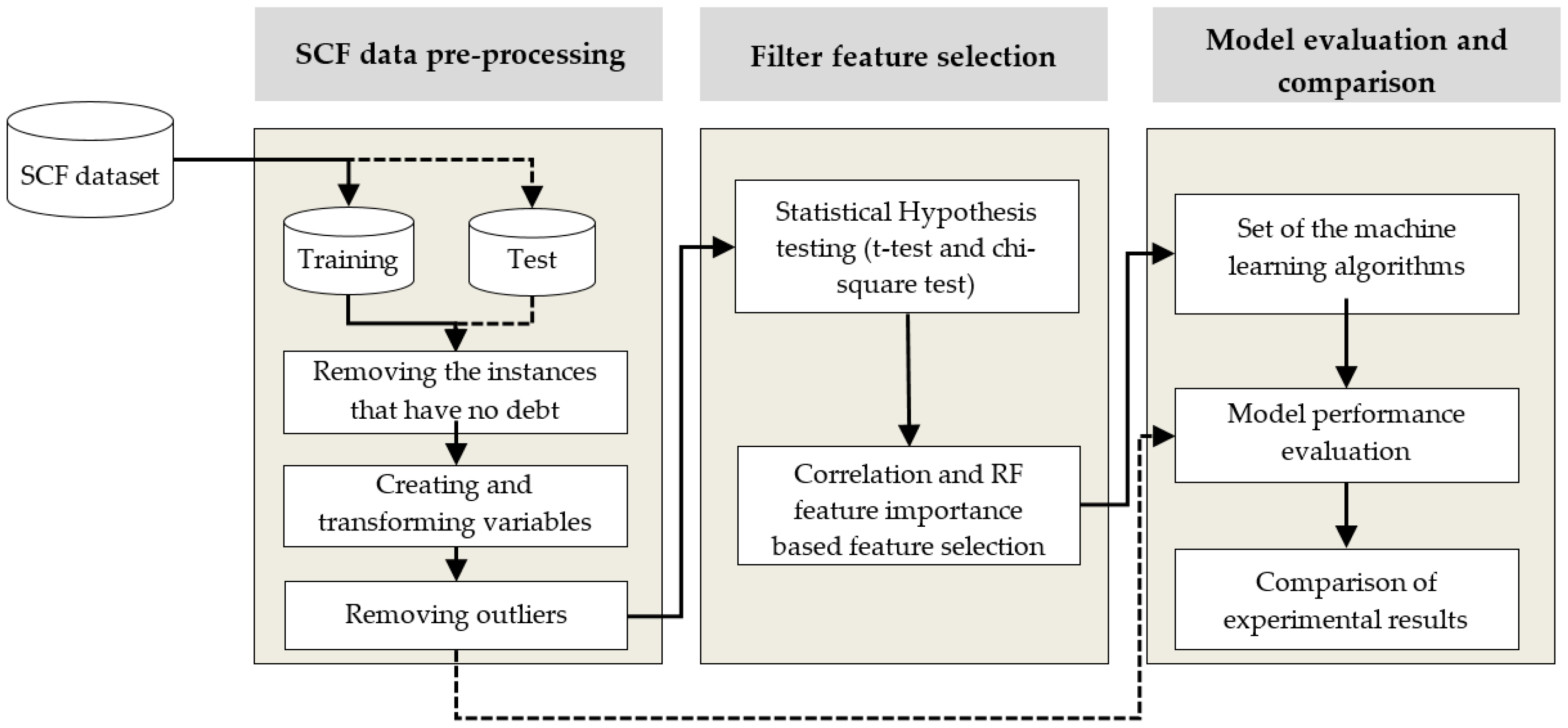
2.1.1. Proposed Framework

The overall architectural diagram of our proposed system design for credit scoring consists of three phases (Figure 1). Firstly, the SCF data is pre-processed. In the second phase, we apply the TSFFS and NAP algorithms to choose the best representative feature subsets that contain the most effective and least redundant variables. In the final phase, the selected feature subsets are used for training machine-learning algorithms to construct credit scoring models. Then we perform an extensive comparison between the machine-learning models and a human expert-based model to determine whether those algorithms can be used in the credit scoring system or not. Machine-learning models trained on the two subsets selected by TSFFS and NAP feature-selection methods are compared with each other to find the appropriate algorithms for credit scoring system as well.

2.1.2. SCF Dataset

The dataset is retrieved from The Federal Reserve’s normally triennial cross-sectional survey of U.S. families [28]. SCF consists of information about families’ balance sheets, pensions, income, demographic characteristics and the borrower’s attitude. Zhang [29] noted that SCF dataset had established an excellent foundation for the household payment problem. Therefore, this dataset is more suitable for the investigation of techniques and methodologies of credit scoring. We used the SCF (1998) as a training set and SCF (2001) as a test set to build credit scoring models. The SCF (1998) and SCF (2001) datasets are summarized in

Table 1. SCF dataset in 1998 and 2001.

Datasets	Good Instances	Bad Instances	Total Instances	Total Variables
Training (SCF-1998)	4113	192	4305	345
Test (SCF-2001)	4245	197	4442	345

; the training and test datasets contain 4113 and 4245 observations, respectively. Each observation contains 345 variables and dependent variable. Surprisingly, from 1983, the SCF survey started to provide information obtained from borrowers about their debt repayment behavior. Prior to the SCF, most information about delinquent debt repayment came from lenders [41]. Therefore, we chose delinquent debt repayment variable (LATE) as a dependent variable. If a household had no late debt payments, the LATE variable is “no” and 0. Otherwise, LATE variable is “yes” and 1. In addition, those panel datasets give the beneficial advantages by evaluating the model trained on the SCF 1998 dataset and tested on the SCF 2001 dataset, as well as discovering new variables can interpret household’s creditworthiness.

2.1.3. A Strategy for Comparing FICO Credit Scores and Machine-Learning Models

In this study, the regression-type algorithm of well-known classification methods is used to estimate the borrowers’ PD. Since the predicted dependent variables are expressed by the probability of borrowers’ creditworthiness, it can be grouped into any number of categories based on the estimated PD. Additionally, when their distributions are equivalent, machine-learning models and FICO credit scores can be compared. Considering that the result of FICO credit scores (

Table 2. U.S distribution of FICO credit scores and probability of default by FICO credit scores from 2000 to 2002.

Credit Rating	FICO Score	The Percent of Population (%)	The Probability of Default (%)	Interest Rate
C1	800 or more	13	1	5.99
C2	750–799	27	1	5.99
C3	700–749	18	4.4	6.21
C4	650–699	15	8.9	6.49
C5	600–649	12	15.8	7.30
C6	550–599	8	22.5	8.94
C7	500–549	5	28.4	9.56
C8	Less than 499	2	41	-

) and SCF data come from the same population, the performance of machine-learning models and FICO scores can be compared [29]. Then the predicted PDs by machine-learning approaches were rationally grouped into eight categories equivalent to the company standard grouping of FICO scores which became de facto. This grouping was made by “Fair, Isaac and Company”, a famous data Analytics Company focused on consumer credit scoring in the U.S [42]. To make a comparison between our performances and FICO credit scores, we use the percent of FICO’s population (column 3 of Table 1) to determine cut-off values to separate credit categories. Then cumulative ECL of each credit category is calculated on the test set.

2.2. Methods

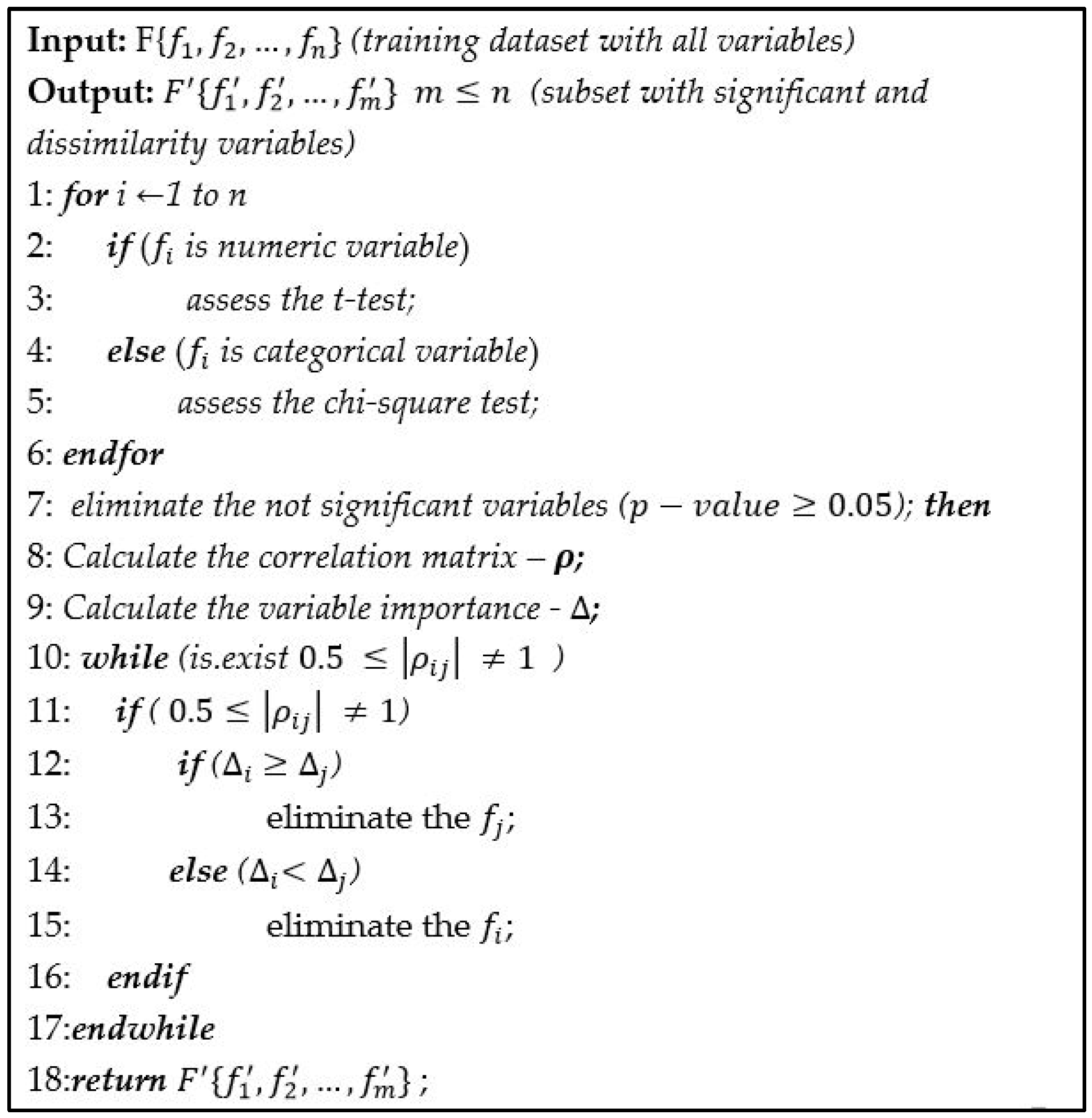
2.2.1. Feature-Selection Algorithms

The investigated survey dataset is high dimensional. Accordingly, we used feature-selection algorithms to reduce the computation cost and choose the most informative variables. In this study, we present TSFFS algorithm and adapt the NAP method for variable-selection.

A two-stage filter feature selection (TSFFS): TSFFS algorithm is implemented in two main steps. In the first step, to avoid redundant and irrelevant variables, we assess the significance of each variable using two hypothesis tests, t-test for continuous variables [43] and chi-square test for categorical variables [44]. In the social sciences, the hypothesis test is generally needed for quantitative research. These hypothesis tests assess whether independent variables provide statistically significant information about clients’ creditworthiness. In other words, for the tested variable, the rejection of the null hypothesis means that the distributions of good and bad borrowers are different. Consequently, the tested variable is believed to have a significant effect on the clients’ creditworthiness.

In the second step, we also eliminate the most unimportant ones from similar variables based on the random forest feature importance and correlation as demonstrated in Figure 2. Random forest-based variable importance is a proper assessment to determine which variables are the most relevant to the dependent variable for both discrete and continuous variables. The correlation coefficient indicates the similarity between the two variables. In this step, if two explanatory variables are highly correlated to each other, we compare the random-forest feature importance for those two variables and choose the most important ones from them. As a result of this step, it is possible to avoid a multicollinearity problem, a situation in which two or more explanatory variables in a multiple regression model are highly linearly related [45]. After selecting variables, the variance inflation factor (VIF) is utilized to quantify the severity of multicollinearity by estimating a score that assesses how much the variance of an estimated regression coefficient is inflated because of multicollinearity in the model [46].

A random forest-based new approach (NAP): this approach for variable selection was presented by Hapfelmeier [38], as an extension of random forest feature-selection algorithm. Although random forest measures variable importance, it cannot answer the question that “Which variables are related to some other independent variables or to the dependent variable?” NAP uses a permutation test framework to assess a null hypothesis of independence between the dependent variable Y and multidimensional vectors of variables X to distinguish relevant from irrelevant variables. The implementation of NAP algorithm:

• Compute random forest importance measure using the training set.
• To assess the empirical distribution of each variable’s random forest importance measure under the null hypothesis, this method permutes each variable separately and several times.
• The p-value is assessed for each variable by means of the empirical distributions and the random forest importance measures.
• Choose the variables with p-value adjusted by Bonferroni-Adjustment lower than a certain threshold.

The authors compared NAP to another eight popular variable-selection methods in three simulation studies and four real data applications. The results showed that NAP provided a higher power to distinguish relevant from irrelevant variables and lead to models which are located among the very best performing ones.

2.2.2. Machine-Learning Approaches

According to Louzada [22], the LR, MARS, SVM, RF, XGBoost and ANN machine-learning approaches are chosen for comparing them to the FICO credit scoring system.

Logistic Regression (LR): Most previous studies compared their own proposed method to the LR in order to demonstrate their methods’ strengths and achievements [6,11,23,47,48,49]. This indicates the LR method can be a benchmark in the credit scoring problem [47]. LR estimates conditional probability of borrower’s default and explains the relationship between clients’ creditworthiness and explanatory variables. The procedure for LR to build a model consists in the estimation of a linear combination between interpreter X and binary dependent variable Y and labeling that converts log-odds to probability using the logistic function. The LR formula is as:

$$Y\approx P(\mathrm{X})=\frac{1}{1+e^{-({\beta }_0+\beta X)}}$$

(1)

The maximum likelihood estimation is usually used to estimate regression coefficients. For each data point, we have interpreter x and binary dependent variable y. The probability of dependent variable is either p(x), if y = 1, or 1 − p(x), if y = 0. Then likelihood is written as:

$$L\left({\beta }_0,\beta \right)={\displaystyle \prod }_{i=1}^{n}p{\left(x_i\right)}^{y_i}{\left(1-p\left(x_i\right)\right)}^{1-y_i}$$

(2)

Advanced machine-learning techniques are quickly gaining applications throughout the financial services industry, transforming the treatment of large and complex datasets, but there is a huge gap between their ability to build powerful predictive models and their ability to understand and manage those models [50]. LR is a phenomenal technique that is commonly used in practice because it satisfies the huge gap as a mentioned above. However, the LR predictability seems to be weaker than other advanced machine-learning algorithms.

Multivariate Adaptive Regression Splines (MARS): This approach has been widely used in modelling problems in the areas of prediction and classification problems [51,52]. Firstly, Lee [11] introduced a two-stage hybrid credit scoring model using the MARS. Although MARS demonstrated the capability of identifying important features, its classification capability was not that good in comparison with MLP neural network. Chuang [53] compared five commonly used credit scoring approaches and demonstrated the advantages of MARS, ANNs and Case Based Reasoning (CBR) to credit analysis. The combination of MARS, ANNs, and CBR methods showed better performance than each individual method, linear discriminant analysis (LDA), LR, classification and regression tree (CART) and ANN.

MARS is a nonlinear and non-parametric regression technique introduced by Friedman [33] for prediction and classification problems. The modelling process of MARS method consists of two phases, the forward and the backward pass. This two-stage approach is based on the "divide and conquers" strategy in which the training sets are partitioned into separate piecewise linear segments (splines) of differing gradients (slope). For interpreter X and binary dependent variable Y, the MARS model, which is a linear combination of basis functions $B_i(x)$ and their interactions, is expressed as:

$$Y=f(x)=c_0+{\displaystyle \sum _{i=1}^k{c}_i}{B}_i(x)$$

(3)

where each $B_i(x)$ is a basis function, k is the number of the basis functions, and each $c_i$ is a constant coefficient.

In the forward pass, MARS repeatedly adds basis function to the model according to a pre-determined maximum reduction in sum-of-squares residual error. After implementing the forward pass, to build a model with better generalization ability, a backward procedure is applied in which the model is pruned by removing those basis functions. It removes the basis functions one by one until it finds the best sub-model. The Generalized Cross-Validation (GCV) error is a criterion to compare the performance of sub-models. It is described as:

$$GCV=\frac{{{\displaystyle \sum }}_{i=1}^n{\left(y_i-f\left(x_i\right)\right)}^2}{\left(1-\frac{C}{n}\right)}$$

(4)

where n is the number of instances in the dataset, C is equal to 1 + cd, d is the effective degrees of freedom (the number of independent basis functions) and c is the penalty for adding a basis function.

Support Vector Machine (SVM): The SVM has been applied in several financial applications recently, mainly in the area of time-series prediction and classification. There are several studies that have applied SVM with various feature-selection methods and hyper-parameters tuning algorithms to credit scoring problem [4,54,55,56]. However, Huang [54] observed SVMs classify credit applications no more accurately than ANN, decision trees or genetic algorithms (GA), and compared the relative importance of using features selected by GA and SVM along with ANN and genetic programming. That study used datasets far smaller and with fewer features than would be used by a financial institution. In this study, we apply SVM to high-dimensional dataset and compare it to other alternative approaches.

The SVM finds a function that has at most ε—insensitive loss deviation from the actually obtained binary dependent variable for each data point [34]. This study briefly describes the case of linear function $f\left(x\right)$ for SVM problem as:

$$f\left(x\right)={\displaystyle \sum }_{i=1}^n{\omega }_i{x}_i+b,\mathrm{with}\omega \in X,b\in R$$

(5)

where $x_i$ is independent variables of n instances with observed binary dependent variable $y_i$. We can write this problem as a convex optimization problem to minimize error, individualizing the hyperplane which maximizes the margin:

$$\begin{array}{l}\mathrm{minimize}\frac{1}{2}{\left|\left|\omega \right|\right|}^2\\ subjectto\{\begin{array}{l}{y}_i-\omega ,x_i-b\le \epsilon \\ \omega ,x_i+b-y_i\le \epsilon \end{array}\end{array}$$

(6)

However, it is possible that there is no existing function $f\left(x\right)$ to provide these constraints for all observations. Analogously to the “soft margin” loss function [57], one can add slack variables ${\xi }_i,{\xi }_n^{*}$ to cope with otherwise infeasible constraints of the optimization problem.

$$\begin{array}{l}\mathrm{minimize}\frac{1}{2}{\left|\left|w\right|\right|}^2+C{\displaystyle {\displaystyle \sum }_{i=1}^n}\left({\xi }_i+{\xi }_n^{*}\right)\\ subjectto\{\begin{array}{c}{y}_i-w,x_i-b\le \epsilon +{\xi }_i\\ w,x_i+b-y_i\le \epsilon +{\xi }_n^{*}\\ {\xi }_i,{\xi }_n^{*}\ge 0\end{array}\end{array}$$

(7)

Parameter C determines the tradeoff between the model complexity and the degree to which deviations larger than $\epsilon$ are tolerated in optimization formulation. This optimization problem can be transformed into the dual problem using Lagrange multipliers and its solution is given by:

$$\mathrm{w}={\displaystyle \sum }_{i=1}^n\left({\alpha }_i-{\alpha }_i^{*}\right)x_{i}thusf\left(x\right)={\displaystyle \sum }_{i=1}^n\left({\alpha }_i-{\alpha }_i^{*}\right)x_i,x+b$$

(8)

where ${\alpha }_i,{\alpha }_i^{*}$ are Lagrange multipliers. We use the Radial basis function (RBF) for SVM regression in this study.

Ensemble Methods: The ensemble procedure applies to methods of combining classifiers, whereby multiple techniques are employed to solve the same problem in order to improve credit scoring performance. There are three popular ensemble approaches: bagging [58], boosting [59], and stacking [60]. Bagging (bootstrap aggregating) technique in which multiple training sets are generated by using bootstrapping, and classifiers are learning for each training set and the predicted class is determined by combining the classification results of each classifier. RF is a bagging algorithm that uses decision trees as the member classifiers.

For credit scoring problem, numerous studies also proposed ensemble classifiers including RF classification [23,61,62,63]. RF often demonstrates better results compared to other machine-learning methods. To estimate borrower’s PD, RF regression is used in this study. This ensemble regression method is built by voting the result of individual regression trees that trained on the diversified subsets from training dataset using bagging by minimizing the mean-squared generalization error (PE*) for any numerical predictors as:

$$PE*=E_{X,Y}{\left(Y-h\left(X\right)\right)}^2$$

(9)

where X, Y are the random vector from the training set, $h\left(X\right)$ is any numerical predictor.

We can define the average generalization error (PE*) of tree as:

$$PE*=E_{\mathsf{\Theta }}{E}_{X,Y}{\left(Y-h\left(X,\mathsf{\Theta }\right)\right)}^2$$

(10)

where Θ is random vector from the training set. Additionally, we can define the average generalization error of forest for all Θ as:

$$P{E}_{forest}^{*}\le \overline{\rho }*{\mathrm{PE}}^{*}$$

(11)

where $\overline{\rho }$ is the weighted correlation between the residuals $Y-h\left(X,\mathsf{\Theta }\right)$ and $Y-h\left(X,{\mathsf{\Theta }}^{\prime }\right)$ are independent.

$$\overline{\rho }=\frac{E_{\mathsf{\Theta }}{E}_{{\mathsf{\Theta }}^{\prime }}\left(\rho \left(\mathsf{\Theta },{\mathsf{\Theta }}^{\prime }\right)sd\left(\mathsf{\Theta }\right)sd\left({\mathsf{\Theta }}^{\prime }\right)\right)}{E_{\mathsf{\Theta }}sd{\left(\mathsf{\Theta }\right)}^2}$$

(12)

where $sd\left(\mathsf{\Theta }\right)=\sqrt{E_{X,Y}{\left(Y-h\left(X,\mathsf{\Theta }\right)\right)}^2}$.

RF also can be used to rank the importance of variables in a regression using internal out-of-bag (OOB) estimates. As mentioned above, this study used OOB estimates for choosing the most important variable from similar variables in the feature-selection procedure.

Furthermore, recently, Xia [23] used XGBoost algorithm with Bayesian hyper-parameter optimization method to construct credit scoring model. They achieved the classification performances compared to other machine-learning methods on the different benchmark credit scoring datasets. XGBoost is a boosting ensemble algorithm; it optimizes the objective of function, size of the tree and the magnitude of the weights are controlled by standard regularization parameters. This method uses CART [64]. Mathematically, K additive function $f_k\left(x\right)$ is used in tree ensemble models to approximate the function $F_K\left(x\right)$, and can be written:

$$Y=F_K(\mathrm{X})={\displaystyle \sum }_{k=1}^K{f}_k\left(x_i\right),f_k\in \mathcal{F}$$

(13)

where K is the number of trees, $x_i$ is the $i$-th training instance and $f_k$ represents a decision rules of the tree and weight of leaf score.

The objective function to be optimized is represented by:

$$L_k(\mathrm{F}({\mathrm{x}}_i))={\displaystyle \sum _{i=1}^n\mathrm{\Psi }({\mathrm{y}}_i,{\mathrm{F}}_K({\mathrm{x}}_i))+{\displaystyle \sum _{k=1}^K\mathrm{\Omega }({\mathrm{f}}_k)}}$$

(14)

where $F_K\left(x_i\right)$ is a prediction on the i-th instance at the K-th boost, $\Psi (\ast )$ is a specified loss function, in terms of regression-type, which can be the mean-squared error function, and $\mathrm{\Omega }\left(f\right)=\gamma T+0.5\times \lambda {\parallel \omega \parallel }^2$ is the regularization term that penalizes the complexity of the model to avoid overfitting problem. In the regularization term, $\gamma$ is the complexity parameter, $\lambda$ is a constant coefficient, ${\parallel \omega \parallel }^2$ is the L2 norm of leaf weights and $T$ denotes the number of leaves. Since XGBoost is trained in an additive manner, the prediction $F_K\left(x_i\right)$ of the $i$-th instance at the $k$-th iteration and it can be written as below:

$$L_k={\displaystyle \sum _{i=1}^n\mathrm{\Psi }({\mathrm{y}}_i,{\mathrm{F}}_{K-1}({\mathrm{x}}_i)+{\mathrm{f}}_k({\mathrm{x}}_i))+{\displaystyle \sum _{k=1}^K\mathrm{\Omega }({\mathrm{f}}_k)}}$$

(15)

The goal of XGBoost is to find the $f_k$ that minimizes the above objective function using gradient descent optimization method.

Artificial Neural Network: Neural networks have been widely used for the credit scoring problem [3,11,48]. Firstly, West [3] applied five different neural network architectures for credit scoring problem. He showed the mixture-of-experts and radial basis function neural network models must be considered for credit scoring application. More recently, different ANNs have been suggested to tackle the credit scoring problem. Namely, probabilistic neural network [65], partial logistic ANN [66], artificial metaplasticity neural network [67] and hybrid neural networks [68]. In some datasets, the neural networks achieve the highest average correct classification rate when compared with other traditional techniques, such as discriminant analysis and LR, taking into account the fact that results were very close [69]. In this study, Multilayer perceptron (MLP) neural network is utilized to construct credit scoring model. MLP is a general architecture in ANN that has been developed to be similar to human brain function (the basic concept of a single perceptron was introduced by Rosenblatt [37]).

MLP consists of three types of layers with completely different roles called input, hidden and output layers. Each layer contains given number of nodes with the activation function and nodes in neighbor layers are linked by weights. The optimal weights are obtained by optimizing objective or loss function using a backpropagation algorithm to build a model as defined:

$$\underset{\omega }{\arg \min }\frac{1}{T}{\displaystyle \sum }_{t}l\left(f\left(\omega x+b\right);y\right)+\lambda \mathrm{\Omega }\left(\omega \right)$$

(16)

where $\omega$ denotes the vector of weights, x is the vector of inputs, b is the bias and $f(\ast )$ is the activation function and $\lambda \mathrm{\Omega }\left(\omega \right)$ is a regularizer. There are several parameters that need to be determined in advance for the training model, such as number of hidden layers, number of their nodes, learning rate, batch size and epoch number.

In a neural network, the choice of optimization algorithm has a significant impact on the training dynamics and task performance. There are many techniques to improve the gradient descent optimization and one of the best optimizers is Adam [70]. Adam computes adaptive learning rates for different parameters from estimates of first and second moments of the gradients and realizes the benefits of both Adaptive Gradient Algorithm and Root Mean Square Propagation. Therefore, Adam is considered one of the best gradient descent optimization algorithms in the field of deep learning because it achieves good results faster than others [71].

In addition, an Early Stopping algorithm is addressed for finding the optimal epoch number based on other given hyper-parameters. This algorithm is to prematurely stop the training at the optimal epoch number when the validation error starts to increase. This also helps to avoid overfitting [72]. However, overfitting is still a challenging issue when the training neural networks are extremely large or working in domains which offer very small amounts of data. If the training neural networks are extremely large, the model will be too complex and it would be transformed into an untrustworthy model.

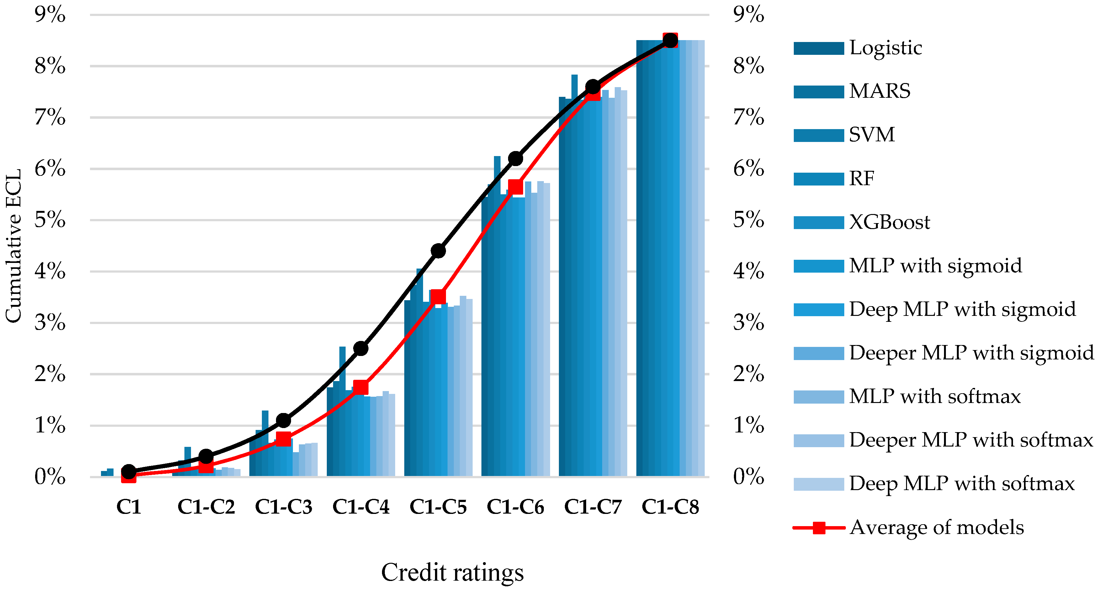
2.2.3. A Cumulative Expected Credit Loss

The goal of evaluation metric is to assess goodness of fit between a given model and the data and is used to generate the model and to compare different machine-learning methods in the context of model selection. The AUC, h-measure, TPR, FPR and accuracy are used to evaluate the ability of machine-learning algorithm to distinguish good and bad borrowers [39].

But in practice, the lending institutions reject or approve the borrowers’ credit application depending on their credit scores. For example, people who have 300–500 credit score on the FICO scores scale of 300-850 are unlikely to get approved for credit cards and other loans because their credit risk is expressed by their credit scoring. Therefore, the cumulative ECL can be one important evaluation metric to measure performance of credit scoring model [40]. We used the cumulative ECL to compare our credit scoring models with FICO scores. In addition, using ECL measurement for model comparison gives the opportunity to choose the credit scoring model with lowest loss and to support decision making to find cut-off credit categories. The cumulative ECL is estimated as following:

1. We estimate PD for each credit category. The PD is the most important major measurement in credit risk modelling used to assess credit losses [73]. It depends on borrower’s individual characteristics and macroeconomic factors such as business cycle, per capita income and unemployment. Furthermore, the PD determines the interest rate for each credit rating as shown in Table 2, creating a link between interest rates and credit risk.

The PD is simply computed by the number of default borrowers divided by the total number of borrowers.

$$PD=\frac{Defaultborrowers}{Totalnumberofborrowers}$$

(17)

2. We can write the formula of ECL for each credit rating as:

$$ECL=EAD*PD*LGD$$

(18)

where EAD is exposure at default and LGD is loss given default. We assume that EAD is expressed by a percentage of population (percent of portfolio) at each credit rating, and LGD can be equal to 1 for consumer loan.

3. Cumulative ECL for credit rating is sum of ECL of all higher credit ratings.

$$CUM\_EC{L}_k={\displaystyle \sum }_{i=1}^{k}EC{L}_i$$

(19)

where $CUM\_EC{L}_k$ is k-th credit rating’s cumulative ECL, $EC{L}_i$ is i-th credit rating’s ECL, k is the number of credit categories.

Assuming that the poor credit scoring model leads to a rise in PD through mispredicting the probability of borrowers’ creditworthiness, cumulative ECL therefore increases. According to this assumption, a lower cumulative ECL indicates better expected performance of the borrowers and it proves that a credit scoring model is more profitable and sustainable.

3. Results

In this section, we will summarize the data pre-processing, experimental setup, result of TSFFS algorithm and comparison of experimental results. In particular, Section 3.4 will present an empirical comparison between machine-learning models and FICO credit scores.

3.1. Data Pre-Processing and Experimental Setup

The data pre-processing, the result of TSFFS algorithm and experimental set-up will be described in this section. Section 3.1.1 will provide the result of data pre-processing such as variable transformation, creation and outlier detection. Then Section 3.1.2 will introduce the process of hyper-parameter tuning for each machine-learning method.

3.1.1. Data Pre-Processing

In data pre-processing, the 1159 instances were dropped from the training set and 1196 from the test set because they have no debt. In addition, the 21 new variables were created because those variables could possibly interpret credit scores well such as total balance of household loan, total number of loan, total number of vehicles, etc. At the outlier detection step, the standard deviation-based outlier detection method was used for finding outliers [74]. The 70 and 127 outliers from training and test sets were dropped because the observed value of those instances were higher than critical value of the log-normal distribution (p-value > 0.05). Finally, the training set contained 2889 (93.9%) good and 187 (6.1%) bad instances, the test set contained 2924 (93.8%) good, 193 (6.2%) bad instances and both datasets consisted of 361 explanatory variables as shown in

Table 3. Pre-processed dataset.

Datasets No.	Good Instances	Bad Instances	Total Instances	Total Variables
Training (SCF-1998)	2889	187	3076	361
Test (SCF-2001)	2924	193	3117	361

.

3.1.2. Experimental Setup

SVM, RF, XGBoost, and MLP methods insist on tuning hyper-parameters to prevent overfitting problem and improve model performance. The grid search with 10-fold cross-validation (GS with 10-fold CV) method is used to find the optimal hyper-parameters for SVM, RF and XGBoost algorithms. GS with 10-fold CV algorithm performs with the given searching space as summarized in

Table 4. Searching space of hyper-parameters.

Method	Parameters	Symbol	Search Space
Support Vector Machine	Gamma	$\gamma$	0.001, 0.01, 0.1
	Cost	$C$	10, 100, 1000
	Epsilon	$\epsilon$	0.05, 0.15, 0.3, 0.5
Random Forest	Number of features randomly sampled	$mtry$	3, 6, 9, 12, 15, 18, 21
	Minimum size of terminal nodes	$nodesize$	50, 80, 110
	Number of tree	$ntree$	500, 1500, 2500
XGBoost	Maximum tree depth	$D_{max}$	2, 4, 6, 8
	Minimum child weight	$w_{mc}$	1, 2, 3, 4
	Early stop round		100
	Maximum epoch number	epoch	500
	Learning rate	$\tau$	0.1
	Number of boost	N	60
	Maximum delta step	$\delta$	0.4,0.6,0.8,1
	Subsample ratio	$r_s$	0.9,0.95,1
	Column subsample ratio	$r_c$	0.9,0.95,1
	Gamma	$\gamma$	0, 0.001

.

For XGBoost and MLP, an Early Stopping algorithm is worked for finding the optimal epoch number based on given other hyper-parameters.

For MLP, the hyper-parameters: learning rate, batch size, and epoch number must be pre-defined to train the model. Since an Early Stopping algorithm is used to find the optimal epoch number, we set the learning rate to 0.0001, maximum epoch number for training to 1000 and use a mini-batch with 32 instances at each iteration. If our algorithm stopped early, a given learning rate and maximum epoch number would be consistent with the training model because our objective function (loss function) that comes from the neural networks is converged before reaching the maximum epoch number.

In this study, we compared six neural networks architectures consisting of different numbers of hidden layers and various activation functions. The first three neural networks used the sigmoid activation function and those are created by one, three, and five hidden layers with eight nodes. The other three neural networks used the ReLU activation function for each hidden layer and the softmax function used for output layer. Those are also built by one, three, and five hidden layers with eight nodes.

All the experiments were performed using the R programming language, 3.4.0 version, on a PC with 3.4 GHz, Intel CORE i7, and 32 GB RAM, using the Microsoft Windows 10 operating system. Particularly, this study used several libraries such as ‘Fselector’, ‘earth’, ‘e1071’, ‘randomForest’, ‘xgboost’ and ‘keras’ in R [75,76,77,78,79,80].

3.2. The Results of Feature-Selection Algorithms

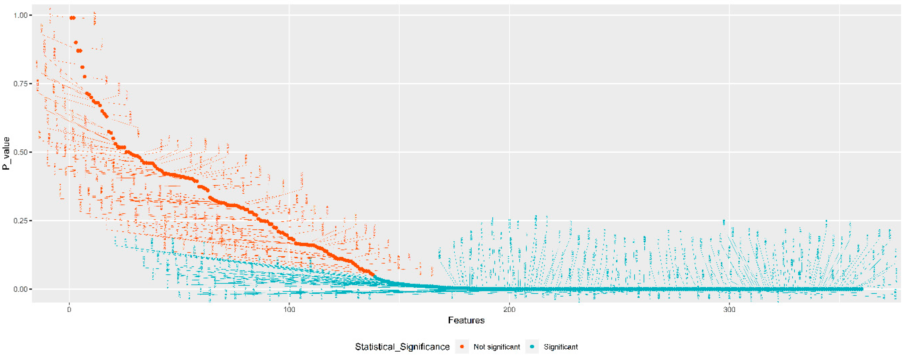
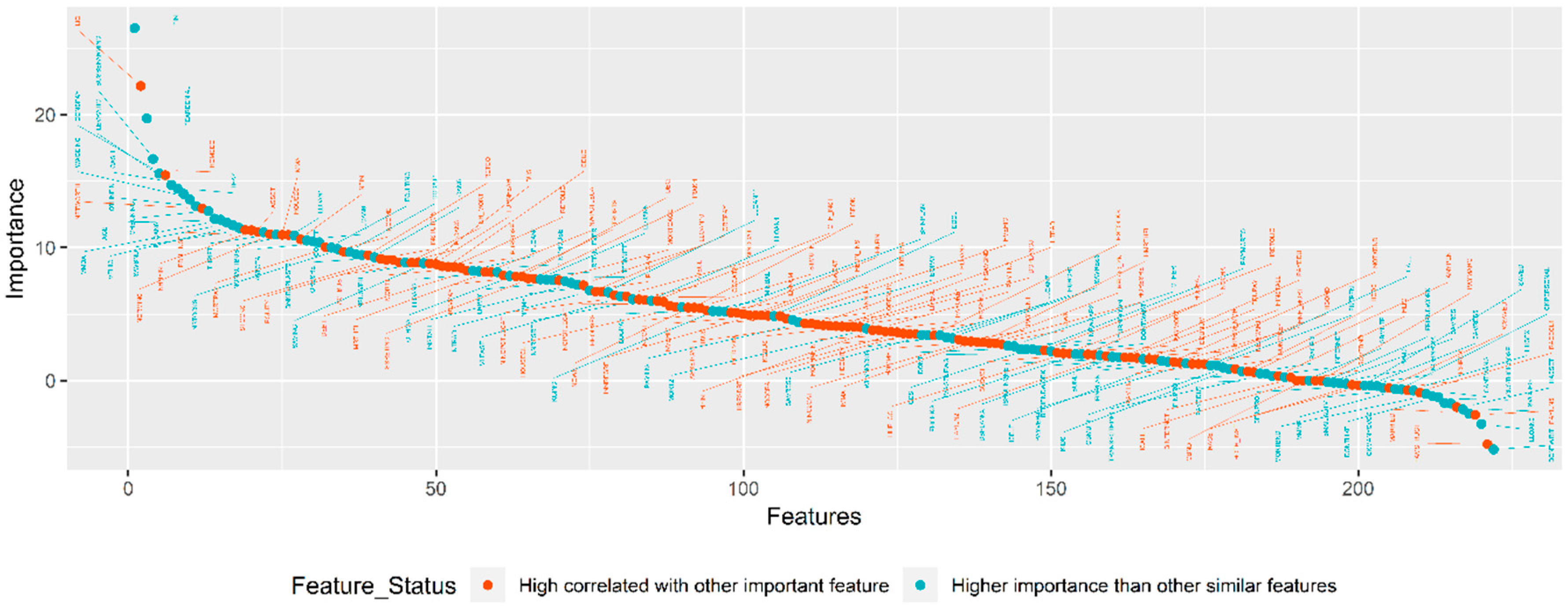
3.2.1. TSFFS Algorithm

In the first step of TSFFS algorithm, we considered statistically significant variables based on the t-test and chi-square test. Regarding the t-test, a two-sample t-test was assessed for continuous variables. For example, the total value of aggregate loan balance for home improvement is not related to a client’s creditworthiness because there is no statistically significant difference between means of bad and good borrowers (p-value = 0.127). For categorical variables, the chi-square test of independence was used to compare frequencies from bad and good borrowers as well. For example, the frequencies of information used for investing decisions (categories: material in mail, TV, radio, advertisements and telemarketer) are similar for both bad and good borrowers (p-value = 0.067). Figure 3 indicates the result of the hypothesis tests, from the left to the right, in which the significance level increases and p-value decreases. At the first step, we have retained 222 variables which are statistically and significantly different for both bad and good borrowers in terms of mean value or frequency. Those variables are represented by cyan points. Other non-significant variables are represented by red points.

In the second step of TSFFS algorithm, the correlation and random forest feature importance were used to choose the most relevant variable from similar variables. As shown in Figure 4, selected variables are denoted by cyan points. The 116 variables were dropped because they have lower importance than other similar variables. In other words, those variables have similar characteristics to the remaining 106 variables. For example, the correlation between total value of financial assets (FIN) and total value of assets (ASSET) is equal to 0.8287, but random forest importance of FIN and ASSET are 10.40 and 4.13, respectively. In this case FIN is chosen because this variable is more important for explaining borrowers’ creditworthiness.

Accordingly, the 106 variables were retained to train the machine-learning model. Those variables match with the part of the information that FICO credit score requires to evaluate the borrower’s credit score such as types of credit, payment history, amounts owed, etc.

Finally, we assessed multicollinearity on the selected variables using VIF based on the logistic regression. VIF is a measure of the independent variable’s collinearity with the other independent variables in the model. In the literature, when VIF values are less than 5 or 10 values, multicollinearity is not an issue in the regression model [81]. Figure 5 shows the result of VIF for each selected variable and according to this, there is no multicollinearity in the model.

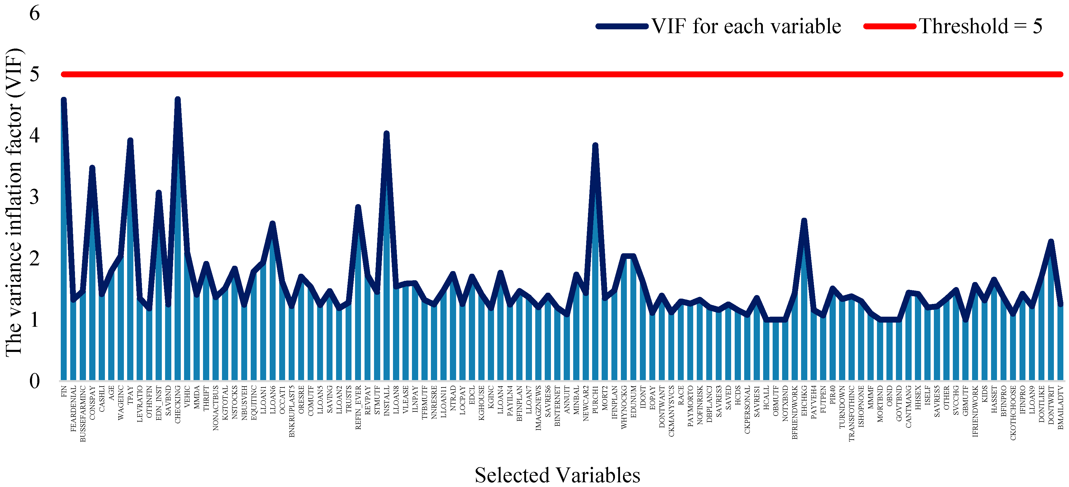
3.2.2. NAP Algorithm

Regarding NAP feature selection, since the SCF dataset consists of a large number of variables, each variable was permuted 10 times to measure random forest importance. Then the p-value adjusted by Bonferroni-Adjustment was assessed and the variables that had a p-value of less than 0.05 were chosen. The NAP method assesses the null hypothesis that needs to be answered as: "Which variables are related to other independent variables or to the dependent variable?" Accordingly, selected variables provide two abilities: a higher predictive strength and being uncorrelated with some other variables. The 76 variables were selected by NAP algorithm and the selected variables by TSFFS and NAP are demonstrated in Tables S1 and S2 in the Supplementary Material.

3.3. Comparison of the Machine-Learning Algorithms

3.3.1. Evaluation Results

This section presents the evaluating models built over various machine-learning algorithms and two feature-selection algorithms. The experiments were looped 10 times to improve their robustness, and the evaluation measures are averaged in the comparison of results.

The main aims of the comparison were to evaluate the effectiveness of the various machine-learning algorithms and to determine the highest performance algorithm. These objectives are valid for variable-selection algorithms as well. The LR, MARS, SVM, RF, XGBoost, and MLP approaches were used to train credit scoring models in the comparison of the experiment. In order to achieve the best performance, hyper-parameters were optimized for each machine-learning method. The results are summarized in

Table 5. The result of machine-learning algorithms.

FS	Machine Learning Models	AUC	H-Measure	TPR	FPR	Accuracy
TSFFS	Logistic	0.8507	0.3880	0.7668	0.2031	0.7950
	MARS	0.8283	0.3591	0.7005	0.1834	0.8094
	SVM	0.7841	0.2429	0.4793	0.1396	0.8368
	RF	0.8544	0.4039	0.8534	0.2709	0.7368
	XGBoost	0.8587	0.3897	0.6192	0.1361	0.8487
	MLP with sigmoid	0.8681	0.4336	0.8259	0.2108	0.7914
	Deep MLP with sigmoid	0.8657	0.4232	0.8135	0.2103	0.7911
	Deeper MLP with sigmoid	0.8581	0.3952	0.7528	0.1915	0.8051
	MLP with softmax	0.8672	0.4243	0.8389	0.2324	0.7720
	Deeper MLP with softmax	0.8637	0.4155	0.7917	0.2115	0.7887
	Deep MLP with softmax	0.8631	0.4128	0.8135	0.2175	0.7844
NAP	Logistic	0.8667	0.4151	0.7762	0.2090	0.7901
	MARS	0.8462	0.3868	0.7166	0.1815	0.8122
	SVM	0.8083	0.3097	0.8788	0.4394	0.5803
	RF	0.8682	0.4214	0.8497	0.2765	0.7313
	XGBoost	0.8633	0.3987	0.5824	0.1163	0.8650
	MLP with sigmoid	0.8726	0.4256	0.8171	0.2337	0.7695
	Deep MLP with sigmoid	0.8718	0.4233	0.8228	0.2303	0.7730
	Deeper MLP with sigmoid	0.8748	0.4298	0.8306	0.2318	0.7720
	MLP with softmax	0.8742	0.4311	0.8358	0.2417	0.7631
	Deeper MLP with softmax	0.8664	0.4126	0.8140	0.2285	0.7742
	Deep MLP with softmax	0.8682	0.4172	0.8161	0.2303	0.7725

and the highest performance for evaluation metrics are bolded.

For the subset selected by the TSFFS algorithm, MLP with sigmoid model indicated the best performance in terms of AUC and h-measure evaluation metrics. This model achieved 86.81% AUC and 0.4336 h-measure, which are 0.09% and 0.01 higher than the second MLP with softmax model trained on the same subset. The AUC indicates classifying ability between borrowers as good and bad, whereas h-measure is better at dealing with cost assumptions among credit classes. In addition, RF and XGBoost models indicated the best performance in terms of TPR, FPR and accuracy. RF model achieved TPR of 85.34%, and XGBoost model achieved FPR of 13.61% and accuracy of 93.81%, thereby outperforming MLP with sigmoid model by 2.8%, 7.5% and 5.7%, respectively.

Regarding NAP variable-selection method, this is better than TSFFS because it improved most evaluation metrics of the best models of TSFFS by 0.7% AUC, 2.5% TPR, 2.0% FPR and 1.6% accuracy. In terms of h-measure, NAP could not improve TSFFS, but it achieved comparable performance for MLP with softmax model. In addition, AUC proves that Deeper MLP with sigmoid model is the best method, indicating it has good separation ability among credit classes. As show in TSFFS subset, XGBoost model outperformed other models in terms of FPR and accuracy.

Overall, it was found that MLP neural networks with sigmoid activation and XGBoost model showed promising results over most evaluation metrics, indicating that these methods are an appropriate approach with NAP variable-selection method in credit scoring.

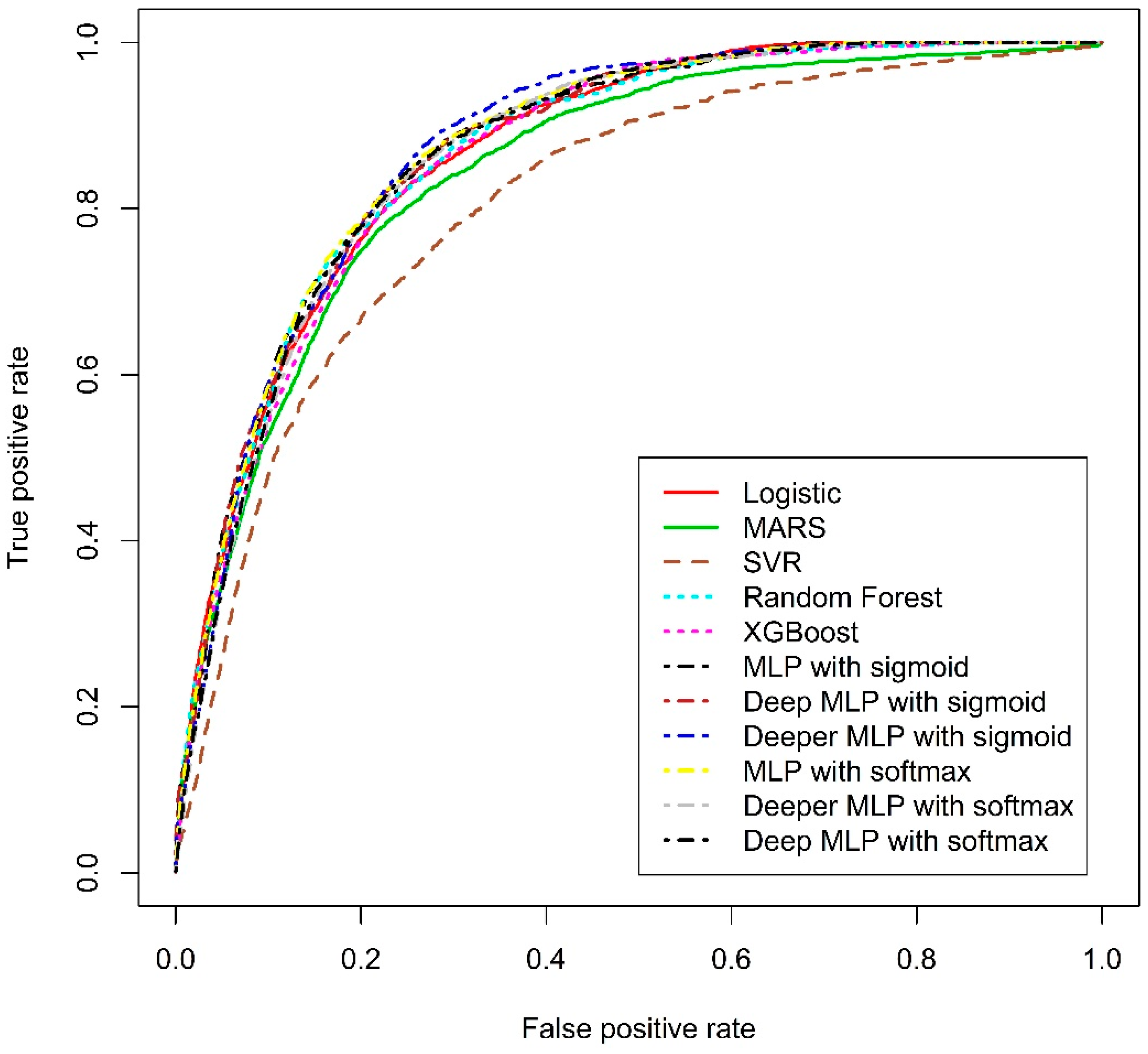
3.3.2. ROC Curve Analysis

The ability of models to distinguish between good and bad borrowers is evaluated using Receiver Operating Characteristic (ROC) curve analysis. The ROC curve is organized by plotting the TPR against FPR over various thresholds. Figure 6 illustrates the ROC curves for the models trained on the subset selected by NAP variable selection. In addition, the calculated TPR and FPR for classifiers can be expressed as an opportunity cost or loan loss for lending institutions [63]. In other words, if lending institutions misclassify good borrowers as bad, refusing to grant loans, it will lead to an opportunity cost. In contrast, in a case where bad borrowers are classified as good borrowers, this creates a loss. For our result, ROC curve of MLP with sigmoid model is higher, which means lower false positive and negative rates than all other algorithms. In other words, if lending institutions used Deeper MLP with sigmoid activation function model trained on the subset selected by NAP variable-selection method to estimate borrowers’ credit scores, their opportunity cost and loan losses would be lower than other models.

From ROC curve analysis, the best credit scoring model is to provide two objectives, which are to maximize TPR (correctly classifying all good borrowers) and minimize FPR (incorrectly classifying all bad borrowers). Since these two objectives cannot be fulfilled comprehensively, lending institutions use multi-class credit scoring as FICO credit scores to balance their profits and losses.

3.4. Empirical Comparison of Machine-Learning Models between FICO

One of the primary objectives of this study is to build a multi-class credit scoring model the same as FICO credit scores and compare them. In this set of experiments, to compare our results with FICO, we applied the percent of FICO’s population which is described in Section 2.1.3 to determine cut-off values for each credit category. In addition, we made 10 times re-sampling from test dataset to construct equivalent distribution as the FICO credit scores as shown in Table 2. Then averaged cumulative ECL was estimated for each model.

Table 6. Cumulative ECL for each credit rating, the comparison between FICO and machine-learning models.

FS	ML Models	C1	C1–C2	C1–C3	C1–C4	C1–C5	C1–C6	C1–C7	C1–C8
TSFFS	Logistic	0.04%	0.33%	0.75%	1.75%	3.89%	6.09%	7.72%	8.50%
	MARS	0.26%	0.47%	0.95%	1.98%	3.93%	6.05%	7.67%	8.50%
	SVM	0.04%	0.64%	1.63%	3.05%	4.76%	6.59%	7.95%	8.50%
	RF	0.02%	0.35%	0.85%	1.56%	3.72%	5.90%	7.51%	8.50%
	XGBoost	0.01%	0.16%	0.69%	1.78%	3.78%	5.89%	7.65%	8.50%
	MLP with sigmoid	0.04%	0.27%	0.66%	1.41%	3.45%	5.81%	7.63%	8.50%
	Deep MLP with sigmoid	0.00%	0.23%	0.74%	1.50%	3.50%	5.67%	7.61%	8.50%
	Deeper MLP with sigmoid	0.00%	0.26%	0.78%	1.73%	3.80%	5.84%	7.58%	8.50%
	MLP with softmax	0.00%	0.26%	0.68%	1.55%	3.38%	5.69%	7.67%	8.50%
	Deeper MLP with softmax	0.00%	0.25%	0.66%	1.61%	3.61%	5.72%	7.63%	8.50%
	Deep MLP with softmax	0.00%	0.26%	0.70%	1.59%	3.52%	5.79%	7.65%	8.50%
	Average of models	0.04%	0.32%	0.83%	1.77%	3.76%	5.91%	7.66%	8.50%
NAP	Logistic	0.00%	0.15%	0.73%	1.74%	3.44%	5.45%	7.40%	8.50%
	MARS	0.11%	0.32%	0.91%	1.86%	3.74%	5.70%	7.36%	8.50%
	SVM	0.16%	0.59%	1.29%	2.53%	4.05%	6.25%	7.83%	8.50%
	RF	0.01%	0.19%	0.66%	1.68%	3.41%	5.50%	7.34%	8.50%
	XGBoost	0.01%	0.15%	0.73%	1.75%	3.64%	5.59%	7.46%	8.50%
	MLP with sigmoid	0.00%	0.21%	0.64%	1.65%	3.29%	5.44%	7.37%	8.50%
	Deep MLP with sigmoid	0.00%	0.17%	0.75%	1.56%	3.39%	5.44%	7.40%	8.50%
	Deeper MLP with sigmoid	0.00%	0.14%	0.48%	1.56%	3.31%	5.75%	7.53%	8.50%
	MLP with softmax	0.00%	0.19%	0.63%	1.57%	3.33%	5.53%	7.38%	8.50%
	Deeper MLP with softmax	0.00%	0.18%	0.65%	1.67%	3.52%	5.75%	7.59%	8.50%
	Deep MLP with softmax	0.00%	0.15%	0.67%	1.61%	3.46%	5.72%	7.53%	8.50%
	Average of models	0.03%	0.22%	0.74%	1.74%	3.51%	5.65%	7.47%	8.50%
FICO		0.10%	0.40%	1.10%	2.50%	4.40%	6.20%	7.60%	8.50%

presents cumulative ECL of our built models on two subsets and FICO credit scores. For variable-selection algorithms, average cumulative ECL of NAP method outperformed TSFFS method the same as theoretical evaluation metrics. Concerning machine-learning methods, XGBoost model could not outperform other models in terms of cumulative ECL. Deeper MLP with sigmoid model, however, achieved the lowest cumulative ECL from C1 rating to C4. In addition, cumulative ECL of FICO credit scores was higher than most machine-learning models between C1 and C7 credit ratings. For both FICO scores and machine-learning models, the cumulative ECLs between C1 and C8 are equal because those models are evaluated by same distribution. This means that machine-learning models can distinguish bad borrowers into C8 credit ratings more than FICO credit scores.

To summarize, if lending institutions approved loan requests of the C1 to C7 credit rating predicted by machine-learning models with NAP variable selection using SCF data, their cumulative ECL would be lower than FICO credit scores (Figure 7). Regarding borrowers who belong to C1–C7 credit rating, MLP with sigmoid activation function model trained on NAP subset indicated the lowest cumulative ECL, which is equal to 7.37%. For other scenarios, Deeper MLP with sigmoid activation function model achieves the lowest cumulative ECL. Nevertheless, this study shows that if lenders in the 2001s used their own credit scoring model built by machine-learning methods instead of FICO credit scores, their cumulative ECL would be lower.

4. Discussion

Credit risk is one of the main fundamental risks a bank or any other financial institution has to meet when operating in the markets. In particular, lending institutions could manage their sustainability as well as financial stability by controlling their credit risk. In order to substantially reduce the potential for credit loss, it is crucial to have a well-designed credit scoring model for bank client credit assessment. In the past, these have been developed by credit experts. Nowadays, machine-learning algorithms have been successfully applied for consumer credit scoring without credit experts. However, previous papers which considered to credit scoring model based on machine-learning approaches have not compared their model to human-based credit scoring model. Therefore, this study compared various machine-learning algorithms to FICO credit scores in order to fill the gap between experimental studies from literature. To do this, we developed a credit scoring model based on SCF dataset using regression-type machine-learning approaches. We also did data pre-processing which were variable creation, transformation and outlier detection.

Most importantly, this study contributed to investigating a more practical model and suggested an effective evaluation metric in order to provide comparisons on real-life application that focuses on consumer credit scoring services. From the results, machine-learning-based credit scoring models outperformed FICO credit scores in terms of cumulative ECL. Then it was observed that if lending institutions in the 2001s used their own credit scoring model constructed by machine-learning approaches with NAP variable-selection algorithm on SCF dataset instead of FICO credit scores, their actual credit losses would be lower and more sustainable. However, it is possible that the results of the empirical comparison may have very slight bias because the estimated PD for the overall population of FICO credit scores is in general different than for those who have debt in sampled SCF data.

5. Conclusions

One of the main focuses of lending institutions is an efficient credit scoring model. In the past, such a model has been developed by human experts, requiring a lot of resources and time. The machine-learning algorithm and artificial intelligence can be used to help the experts and reduce labour. This study compared the state-of-the-art machine-learning approaches with two variables selection algorithm and FICO credit scores by establishing the U.S. families’ survey data as a practical benchmark data.

We built regression models to estimate borrowers’ probability of default and adapted effective evaluation metrics in order to provide an extensive comparison between the real-life application and theoretical models. The main conclusions from the comparison are that machine-learning models showed better performance compared to FICO credit scoring in 2001s. Additionally, the deep neural networks and XGBoost models demonstrated the promising performances compared with other machine-learning approaches in terms of AUC and accuracy. XGBoost model achieved the best accuracy, but it could not show good performance for cumulative ECL. This means that although accuracy is the most appropriate measure for evaluating the classification performance, it is inadequate to evaluate the ability of the credit scoring model. In the case of AUC, it is not compatible with cumulative ECL as well. It is shown that theoretical performance measures are inappropriate for evaluating the credit scoring model. Therefore, it is important to use the measure of business reality of credit scoring when comparing the credit scoring models. According to cumulative ECL, the deep neural networks are an appropriate approach for credit scoring system. However, the deep neural network approach has been useless because of its black box nature, so the relationship between input and output cannot be completely understood. Therefore, this area requires further research to investigate this explanation for credit scoring. In addition, the feature-selection approaches explored in this work have also contributed to the final performance, since the SCF dataset is non-synthetic and thus noisy. NAP variable-selection method confirmed itself as a suitable algorithm for selecting the most relevant variables from high-dimensional social survey data.

We anticipate potential future work in this area that includes developing other machine-learning algorithms for credit scoring as well as novel approaches for feature selection based on the SCF dataset.

References

1. Chang, H.; Park, M.A. Smart e-Form for Effective Business Communication in the Financial Industry. Bus. Commun. Res. Pract. 2018, 1, 95–101. [Google Scholar] [CrossRef]
2. Altman, E.I. Financial ratios, discriminant analysis and the prediction of corporate bankruptcy. J. Financ. 1968, 23, 589–609. [Google Scholar] [CrossRef]
3. West, D. Neural network credit scoring models. Comput. Oper. Res. 2000, 27, 1131–1152. [Google Scholar] [CrossRef]
4. Huang, Z.; Chen, H.; Hsu, C.J.; Chen, W.H.; Wu, S. Credit rating analysis with support vector machines and neural networks: A market comparative study. Decis. Support Syst. 2004, 37, 543–558. [Google Scholar] [CrossRef]
5. Thomas, L.C. A survey of credit and behavioural scoring: Forecasting financial risk of lending to consumers. Int. J. Forecast. 2000, 16, 149–172. [Google Scholar] [CrossRef]
6. Orgler, Y.E. A credit scoring model for commercial loans. J. Money Credit Bank. 1970, 2, 435–445. [Google Scholar] [CrossRef]
7. Hoffmann, F.; Baesens, B.; Mues, C.; Van Gestel, T.; Vanthienen, J. Inferring descriptive and approximate fuzzy rules for credit scoring using evolutionary algorithms. Eur. J. Oper. Res. 2007, 177, 540–555. [Google Scholar] [CrossRef]
8. Oreski, S.; Oreski, G. Genetic algorithm-based heuristic for feature selection in credit risk assessment. Expert Syst. Appl. 2014, 41, 2052–2064. [Google Scholar] [CrossRef]
9. Giudici, P. Bayesian data mining, with application to benchmarking and credit scoring. Appl. Stoch. Models Bus. Ind. 2001, 17, 69–81. [Google Scholar] [CrossRef]
10. Lee, T.S.; Chiu, C.C.; Lu, C.J.; Chen, I.F. Credit scoring using the hybrid neural discriminant technique. Expert Syst. Appl. 2002, 23, 245–254. [Google Scholar] [CrossRef]
11. Lee, T.S.; Chen, I.F. A two-stage hybrid credit scoring model using artificial neural networks and multivariate adaptive regression splines. Expert Syst. Appl. 2005, 28, 743–752. [Google Scholar] [CrossRef]
12. Wang, G.; Ma, J.; Huang, L.; Xu, K. Two credit scoring models based on dual strategy ensemble trees. Knowl. Based Syst. 2012, 26, 61–68. [Google Scholar] [CrossRef]
13. Liu, Y.; Schumann, M. Data mining feature selection for credit scoring models. J. Oper. Res. Soc. 2005, 56, 1099–1108. [Google Scholar] [CrossRef]
14. Bellotti, T.; Crook, J. Support vector machines for credit scoring and discovery of significant features. Expert Syst. Appl. 2009, 36, 3302–3308. [Google Scholar] [CrossRef] [Green Version]
15. Wang, C.M.; Huang, Y.F. Evolutionary-based feature selection approaches with new criteria for data mining: A case study of credit approval data. Expert Syst. Appl. 2009, 36, 5900–5908. [Google Scholar] [CrossRef]
16. Chen, F.L.; Li, F.C. Combination of feature selection approaches with SVM in credit scoring. Expert Syst. Appl. 2010, 37, 4902–4909. [Google Scholar] [CrossRef]
17. Waad, B.; Ghazi, B.M.; Mohamed, L. A three-stage feature selection using quadratic programming for credit scoring. Appl. Artif. Intell. 2013, 27, 721–742. [Google Scholar] [CrossRef]
18. Yeh, I.C.; Lien, C.H. The comparisons of data mining techniques for the predictive accuracy of probability of default of credit card clients. Expert Syst. Appl. 2009, 36, 2473–2480. [Google Scholar] [CrossRef]
19. Kieso, D.E.; Weygandt, J.J.; Warfield, T.D. Intermediate Accounting: IFRS Edition; John Wiley & Sons: Hoboken, NJ, USA, 2010. [Google Scholar]
20. Basel Committee. Basel III: A Global Regulatory Framework for More Resilient Banks and Banking Systems; Basel Committee: Basel, Switzerland, 2010. [Google Scholar]
21. Asuncion, A.; Newman, D. UCI Machine Learning Repository. Available online: http://www.ics.uci.edu/~mlearn/MLRepository.html (accessed on 1 November 2018).
22. Louzada, F.; Ara, A.; Fernandes, G.B. Classification methods applied to credit scoring: Systematic review and overall comparison. Comput. Oper. Res. 2016, 21, 117–134. [Google Scholar] [CrossRef] [Green Version]
23. Xia, Y.; Liu, C.; Li, Y.; Liu, N. A boosted decision tree approach using Bayesian hyper-parameter optimization for credit scoring. Expert Syst. Appl. 2017, 78, 225–241. [Google Scholar] [CrossRef]
24. Chen, Q.; Tsai, S.B.; Zhai, Y.; Chu, C.C.; Zhou, J.; Li, G.; Hsu, C.F. An Empirical Research on Bank Client Credit Assessments. Sustainability 2018, 10, 1406. [Google Scholar] [CrossRef]
25. Dinh, T.H.; Kleimeier, S. A credit scoring model for Vietnam’s retail banking market. Int. Rev. Financ. Anal. 2007, 16, 471–495. [Google Scholar] [CrossRef]
26. Jacobson, T.; Roszbach, K. Bank lending policy, credit scoring and value-at-risk. J. Bank. Financ. 2003, 27, 615–633. [Google Scholar] [CrossRef] [Green Version]
27. Zhou, G.; Zhang, Y.; Luo, S. P2P Network Lending, Loss Given Default and Credit Risks. Sustainability 2018, 10, 1010. [Google Scholar] [CrossRef]
28. Bucks, B.K.; Kennickell, A.B.; Moore, K.B. Recent changes in US family finances: Evidence from the 2001 and 2004 Survey of Consumer Finances. Fed. Res. Bull. 2006, A1, 92. [Google Scholar]
29. Zhang, T.; DeVaney, S.A. Determinants of consumer’s debt repayment patterns. Consum. Interest Annu. 1990, 45, 65–70. [Google Scholar]
30. Board of Governors of the Federal Reserve System (US). Report to the Congress on Credit Scoring and its Effects on the Availability and Affordability of Credit, Board of Governors of the Federal Reserve System. Available online: https://www.federalreserve.gov/boarddocs/rptcongress/creditscore/creditscore.pdf (accessed on 26 January 2019).
31. Arezzo, M.F.; Guagnano, G. Response-Based Sampling for Binary Choice Models with Sample Selection. Econometrics 2018, 6, 12. [Google Scholar] [CrossRef]
32. Cox, D.R. The regression analysis of binary sequences. J. R. Stat. Soc. Ser. B Stat. Methodol. 1958, 20, 215–242. [Google Scholar] [CrossRef]
33. Friedman, J.H. Multivariate adaptive regression splines. Ann. Stat. 1991, 33, 1–67. [Google Scholar] [CrossRef]
34. Cortes, C.; Vapnik, V. Support-vector networks. Mach. Learn. 1995, 20, 273–297. [Google Scholar] [CrossRef] [Green Version]
35. Breiman, L. Random forests. Mach. Learn. 2001, 45, 5–32. [Google Scholar] [CrossRef]
36. Chen, T.; Guestrin, C. Xgboost: A scalable tree boosting system. arXiv, 2016; arXiv:1603.02754. [Google Scholar]
37. Rosenblatt, F. The perceptron: A probabilistic model for information storage and organization in the brain. Psychol. Rev. 1958, 65, 386. [Google Scholar] [CrossRef] [PubMed]
38. Hapfelmeier, A.; Ulm, K. A new variable selection approach using random forests. Comput. Stat. Data Anal. 2013, 60, 50–69. [Google Scholar] [CrossRef]
39. Hand, D.J.; Anagnostopoulos, C. A better Beta for the H measure of classification performance. Pattern Recognit. Lett. 2014, 40, 41–46. [Google Scholar] [CrossRef]
40. Volareviþ, H.; Varoviþ, M. Internal model for ifrs 9-expected credit losses calculation. Ekonomski Pregled 2018, 69, 269–297. [Google Scholar] [CrossRef]
41. DeVaney, S.A.; Lytton, R.H. Household insolvency: A review of household debt repayment, delinquency, and bankruptcy. Financ. Serv. Rev. 1995, 4, 137–156. [Google Scholar] [CrossRef] [Green Version]
42. Sengupta, R.; Bhardwaj, G. Credit scoring and loan default. Int. Rev. Financ. 2015, 15, 139–167. [Google Scholar] [CrossRef]
43. Welch, B.L. The significance of the difference between two means when the population variances are unequal. Biometrika 1938, 29, 350–362. [Google Scholar] [CrossRef]
44. Bhapkar, V.P. A note on the equivalence of two test criteria for hypotheses in categorical data. J. Am. Stat. Assoc. 1966, 61, 228–235. [Google Scholar] [CrossRef]
45. Farrar, D.E.; Glauber, R.R. Multicollinearity in regression analysis: The problem revisited. Rev. Econ. Stat. 1967, 92–107. [Google Scholar] [CrossRef]
46. Belsley, D.A. A guide to using the collinearity diagnostics. Comput. Sci. Econ. Manag. 1991, 4, 33–50. [Google Scholar]
47. Lessmann, S.; Baesens, B.; Seow, H.V.; Thomas, L.C. Benchmarking state-of-the-art classification algorithms for credit scoring: An update of research. Eur. J. Oper. Res. 2015, 247, 124–136. [Google Scholar] [CrossRef] [Green Version]
48. Kim, Y.S.; Sohn, S.Y. Managing loan customers using misclassification patterns of credit scoring model. Expert Syst. Appl. 2004, 26, 567–573. [Google Scholar] [CrossRef]
49. Van Gestel, T.; Baesens, B.; Van Dijcke, P.; Suykens, J.; Garcia, J.; Alderweireld, T. Linear and nonlinear credit scoring by combining logistic regression and support vector machines. J. Credit Risk 2005, 1. [Google Scholar] [CrossRef]
50. Vellido, A.; Martín-Guerrero, J.D.; Lisboa, P.J. Making machine learning models interpretable. ESANN 2012, 12, 163–172. [Google Scholar]
51. De Gooijer, J.G.; Ray, B.; Kräger, H. Forecasting exchange rates using TSMARS. J. Int. Money Financ. 1998, 17, 513–534. [Google Scholar] [CrossRef] [Green Version]
52. Kuhnert, P.M.; Do, K.A.; McClure, R. Combining non-parametric models with logistic regression: An application to motor vehicle injury data. Comput. Stat. Data Anal. 2000, 34, 371–386. [Google Scholar] [CrossRef]
53. Chuang, C.L.; Lin, R.H. Constructing a reassigning credit scoring model. Expert Syst. Appl. 2009, 36, 1685–1694. [Google Scholar] [CrossRef]
54. Huang, C.L.; Chen, M.C.; Wang, C.J. Credit scoring with a data mining approach based on support vector machines. Expert Syst. Appl. 2007, 33, 847–856. [Google Scholar] [CrossRef] [Green Version]
55. Han, L.; Han, L.; Zhao, H. Orthogonal support vector machine for credit scoring. Eng. Appl. Artif. Intell. 2013, 26, 848–862. [Google Scholar] [CrossRef]
56. Shi, J.; Xu, B. Credit scoring by fuzzy support vector machines with a novel membership function. J. Risk Financ. Manag. 2016, 9, 13. [Google Scholar] [CrossRef]
57. Bennett, K.P.; Mangasarian, O.L. Robust linear programming discrimination of two linearly inseparable sets. Optim. Methods Softw. 1992, 1, 23–34. [Google Scholar] [CrossRef] [Green Version]
58. Breiman, L. Bagging predictors. Mach. Learn. 1996, 24, 123–140. [Google Scholar] [CrossRef] [Green Version]
59. Schapire, R.E. The strength of weak learnability. Mach. Learn. 1990, 5, 197–227. [Google Scholar] [CrossRef] [Green Version]
60. Wolpert, D.H. Stacked generalization. Neural Netw. 1992, 5, 241–259. [Google Scholar] [CrossRef] [Green Version]
61. Kruppa, J.; Schwarz, A.; Arminger, G.; Ziegler, A. Consumer credit risk: Individual probability estimates using machine learning. Expert Syst. Appl. 2013, 40, 5125–5131. [Google Scholar] [CrossRef]
62. Koutanaei, F.N.; Sajedi, H.; Khanbabaei, M. A hybrid data mining model of feature selection algorithms and ensemble learning classifiers for credit scoring. J. Retail. Consum. Serv. 2015, 27, 11–23. [Google Scholar] [CrossRef]
63. Ala’raj, M.; Abbod, M.F. Classifiers consensus system approach for credit scoring. Knowl. Based Syst. 2016, 104, 89–105. [Google Scholar] [CrossRef] [Green Version]
64. Breiman, L. Classification and Regression Trees; Routledge: London, UK, 2017. [Google Scholar]
65. Su-lin, P.A. Study on Credit Scoring Model and Forecasting Based on Probabilistic Neural Network. Syst. Eng.-Theory Pract. 2005, 5, 006. [Google Scholar]
66. Lisboa, P.J.; Etchells, T.A.; Jarman, I.H.; Arsene, C.T.; Aung, M.H.; Eleuteri, A.; Taktak, A.F.; Ambrogi, F.; Boracchi, P.; Biganzoli, E. Partial logistic artificial neural network for competing risks regularized with automatic relevance determination. IEEE Trans. Neural Netw. 2009, 20, 1403–1416. [Google Scholar] [CrossRef] [PubMed]
67. Marcano-Cedeno, A.; Marin-De-La-Barcena, A.; Jiménez-Trillo, J.; Pinuela, J.A.; Andina, D. Artificial metaplasticity neural network applied to credit scoring. Int. J. Neural Syst. 2011, 21, 311–317. [Google Scholar] [CrossRef]
68. Chuang, C.L.; Huang, S.T. A hybrid neural network approach for credit scoring. Expert Syst. 2011, 28, 185–196. [Google Scholar] [CrossRef]
69. Abdou, H.; Pointon, J.; El-Masry, A. Neural nets versus conventional techniques in credit scoring in Egyptian banking. Expert Syst. Appl. 2008, 35, 1275–1292. [Google Scholar] [CrossRef] [Green Version]
70. Kingma, D.P.; Ba, J. Adam: A method for stochastic optimization. arXiv, 2014; arXiv:1412.6980. [Google Scholar]
71. Ruder, S. An overview of gradient descent optimization algorithms. arXiv, 2016; arXiv:1609.04747. [Google Scholar]
72. Girosi, F.; Jones, M.; Poggio, T. Regularization theory and neural networks architectures. Neural Comput. 1995, 7, 219–269. [Google Scholar] [CrossRef]
73. Alam, M.; Hao, C.; Carling, K. Review of the literature on credit risk modeling: Development of the past 10 years. Banks Bank Syst. 2010, 5, 43–60. [Google Scholar]
74. Dixon, W.J. Processing data for outliers. Biometrics 1953, 9, 74–89. [Google Scholar] [CrossRef]
75. Romanski, P.; Kotthoff, L.; Kotthoff, M.L. Package ‘FSelector’. 2013. Available online: http://cran/r-project. org/web/packages/FSelector/index. html (accessed on 16 May 2018).
76. Dimitriadou, E.; Hornik, K.; Leisch, F.; Meyer, D.; Weingessel, A.; Leisch, M.F. Package ‘e1071’. R Software package. 2009. Available online: http://cran.rproject.org/web/packages/e1071/index.html (accessed on 21 January 2019).
77. Liaw, A.; Wiener, M. The randomforest package. R News 2002, 2, 18–22. [Google Scholar]
78. Chen, T.; He, T.; Benesty, M. Xgboost: Extreme Gradient Boosting. R package Version. Available online: https://cran.r-project.org/web/packages/xgboost/vignettes/xgboostPresentation.html (accessed on 9 June 2018).
79. Arnold, T. kerasR: R Interface to the Keras Deep Learning Library. Computer Software Manual (R Package Version 0.6. 1). Available online: https://CRAN.R-project.org/package=kerasR (accessed on 22 November 2018).
80. Sing, T.; Sander, O.; Beerenwinkel, N.; Lengauer, T. ROCR: Visualizing classifier performance in R. Bioinformatics 2005, 21, 3940–3941. [Google Scholar] [CrossRef]
81. O’brien, R.M. A caution regarding rules of thumb for variance inflation factors. Qual. Quant. 2007, 41, 673–690. [Google Scholar] [CrossRef]
Figure 1. System design for credit scoring. SCF—Survey of Consumer Finances and RF-Random Forest.
Sustainability 11 00699 g001
Figure 2. Pseudocode of the TSFFS feature-selection algorithm.
Sustainability 11 00699 g002
Figure 3. The results of hypothesis tests.
Sustainability 11 00699 g003
Figure 4. The result of feature selection using RF feature importance and correlation.
Sustainability 11 00699 g004
Figure 5. The variance inflation factor for selected variables.
Sustainability 11 00699 g005
Figure 6. ROC curve comparing the model performances on the subset selected by NAP variable selection method.
Sustainability 11 00699 g006
Figure 7. Cumulative ECL comparing machine-learning model performances on NAP subset and FICO.
Sustainability 11 00699 g007