Article

Estimation of Soil Organic Matter, Total Nitrogen and Total Carbon in Sustainable Coastal Wetlands

1
School of Geomatics and Marine Information, Huaihai Institute of Technology, Lianyungang 222005, China
2
Jiangsu Coastal Zone Environment Research Institute, Lianyungang 222005, China
3
National Astronomical Observatories, Key Lab of Lunar Science and Deep-exploration, Chinese Academy of Sciences, Beijing 100101, China
4
School of Resources and Environment, Henan University of Economics and Law, Zhengzhou 450002, China
*
Authors to whom correspondence should be addressed.
Sustainability 2019, 11(3), 667; https://doi.org/10.3390/su11030667
Submission received: 30 November 2018 / Revised: 11 January 2019 / Accepted: 17 January 2019 / Published: 28 January 2019
(This article belongs to the Special Issue Soil Erosion and the Sustainable Management of the Landscape)

Abstract

:
Soil plays an important role in coastal wetland ecosystems. The estimation of soil organic matter (SOM), total nitrogen (TN), and total carbon (TC) was investigated at the topsoil (0–20 cm) in the coastal wetlands of Dafeng Elk National Nature Reserve in Yancheng, Jiangsu province (China) using hyperspectral remote sensing data. The sensitive bands corresponding to SOM, TN, and TC content were retrieved based on the correlation coefficient after Savitzky–Golay (S–G) filtering and four differential transformations of the first derivative (R′), first derivative of reciprocal (1/R)′, second derivative of reciprocal (1/R)″, and first derivative of logarithm (lgR)′ by spectral reflectance (R) as R′, (1/R)′, (1/R)″, (lgR)′ of soil samples. The estimation models of SOM, TN, and TC by support vector machine (SVM) and back propagation (BP) neural network were applied. The results indicated that the effective bands can be identified by S–G filtering, differential transformation, and the correlation coefficient methods based on the original spectra of soil samples. The estimation accuracy of SVM is better than that of the BP neural network for SOM, TN, and TC in the Yancheng coastal wetland. The estimation model of SOM by SVM based on (1/R)′ spectra had the highest accuracy, with the determination coefficients (R2) and root mean square error (RMSE) of 0.93 and 0.23, respectively. However, the estimation models of TN and TC by using the (1/R)″ differential transformations of spectra were also high, with determination coefficients R2 of 0.88 and 0.85, RMSE of 0.17 and 0.26, respectively. The results also show that it is possible to estimate the nutrient contents of topsoil from hyperspectral data in sustainable coastal wetlands.

1. Introduction

The organic matter in wetland soil is not only an important source of surface soil organic carbon, but also an important indicator for judging the soil fertility of wetlands [1]. Nitrogen is the most important limiting nutrient in wetland soils and a sensitive indicator for measuring the soil nutrient levels in wetlands [2]. The carbon in the wetland soil is mainly produced by plants that fix the carbon in the atmosphere through photosynthesis, and it is an important factor that affects greenhouse gas emissions [3]. Therefore, determining the contents of soil organic matter (SOM), total nitrogen (TN) and total carbon (TC) in wetland soil is of great significance for protecting the wetland ecological environment [4]. Traditional methods for the analysis of nutrient contents in soil are mainly based on chemical analysis, which is time consuming and labor-intensive. Hence, the emergence of the hyper-spectral remote sensing technique makes up for the shortcomings of traditional laboratory methods, and can provide a strong technical support for the estimation of soil nutrients.
There are three main steps in estimating the nutrient contents in soil by the hyper-spectral remote sensing technique: Firstly, the obtained raw spectral data is preprocessed to eliminate or attenuate noise in the original reflectance spectra and to amplify useful spectral information. The common pretreatment methods include the successive projections algorithm (SPA) [5,6], the Savitzky–Golay filter [7,8], multiplicative scattering correction (MSC) [9,10], the integration algorithm (IA) [11,12], wavelet transform (WT) [13,14], and exponential transformation (RI, NDI, DI) [15]. Secondly, the pre-processed spectra are used to retrieve characteristic bands, which are sensitive to the nutrients in soil. Commonly used methods are mainly the correlation coefficient method [16,17], stepwise regression method, and the genetic algorithm [18,19]. Thirdly, the spectral data of the characteristic bands and the corresponding physical and chemical soil data are used to construct the estimation models. Current methods are mainly divided into linear and nonlinear models. Linear modeling methods mainly include multiple linear regression [20,21], linear regression [22], partial least squares regression [23,24], and principal component regression [25,26]. Nonlinear modeling methods mainly include the back propagation (BP) neural network [27,28], least squares support vector machine (LS-SVM) [29,30].
Up to date, some researchers have used linear and non-linear models to estimate SOM, TN and TC contents. For example, Dalal and Henry [31] studied the relationship between soil spectra and nitrogen at 1100–2500 nm, the appropriate prediction band (1700–2100 nm) was selected by multiple regression analysis, and the prediction model was constructed. Zhang [32] used the partial least squares (PLS)-BP neural network, PLS and spectral index methods to estimate the TN content of different types of soils, and found that the prediction of neural network model was better than partial least squares model. Yu et al. [33] took the soil of Hanjiang River plain as the research object, and established the prediction model of SOM in this region based on the full band (400–2400 nm) and the significant band by using partial least squares regression (PLSR). The results showed that the prediction model precision based on the CR-PLSR (continuum removal PLSR) algorithm was more significant than that based on R-PLSR (raw spectral reflectance PLSR), LR-PLSR (inverse-log reflectance PLSR), and FDR-PLSR (first order differential reflectance PLSR) models. Bao et al. [34] comprehensively analyzed the relationship between the SOM content and the corresponding spectral reflectance of different soils, then used PLS and PLS-SVM (support vector machine) methods to predict the SOM content in mining areas, and found that PLS-SVM is more accurate than PLS. Zhang et al. [35] estimated SOM and available potassium by using partial least squares (PLS) and least squares support vector machine (LS-SVM). Numerous studies have concentrated on modeling soil parameters from remote sensing techniques either from bare soil, or by inferring soil properties by vegetation cover [36,37]. However, applying hyper-spectral remote sensing technology to the topsoil nutrients in coastal wetlands remains limited [38]. Coastal wetlands, as an ecosystem between land and water, are greatly influenced by the marine environment and exhibit unique soil characteristics. Taking the coastal wetland soil of Dafeng Elk Wild Pastoral Area of Jiangsu Province as the research object, the modeling method of the nonlinear model support vector machine (SVM) and BP neural network algorithm were applied to estimate SOM, TN, and TC of the topsoil in coastal wetlands.
The goal of this study is to develop the statistical models that estimate SOM, TN, and TC from the hyper-spectral remote sensing of 34 topsoil samples (0–20 cm), providing a rapid and practical method to remotely monitor soil nutrients in coastal wetland environments. We hypothesized that soil properties can be inferred by reflectance spectra. The characteristic bands of SOM based on transformations (1/R)′ were 498–501 nm, 1180–1182 nm, 1946 nm, 1947 nm, 2323–2326 nm; characteristic bands of soil TN based on transformations (1/R)″ were 536 nm, 900 nm, 1177 nm, 1178 nm, 1285–1287 nm, 1977 nm, 2319–2322 nm, 2345 nm, 2346 nm; and the characteristic bands of soil TC based on transformations (1/R)″ are 536–537 nm, 561–562 nm, 619–622 nm, 899–900 nm, 1234–1235 nm, 1438–1439 nm, 1795–1796 nm, 1949–1952 nm, 2345–2347 nm, 2373 nm respectively. Our research can expand the feasibility of the non-linear hyper-spectral estimation model for SOM, TN, and TC content in coastal wetland soils, and lay a foundation for further research on the theory and model of the hyperspectral remote sensing image estimation of soil nutrients in coastal wetlands.

2. Materials and Methods

2.1. Study Area

The Dafeng Elk National Nature Reserve is located in the Jiangsu Province and south of Yellow Sea Wetland at 32°59′–33°03′ N and 120°47′–120°53′ E, and is one of four wetlands in China (South Yellow Sea Wetland, Qinghai-Tibet Plateau Wetland, Northeast Sanjiang Plain Wetland, and Poyang Lake Wetland) (Figure 1). The total coverage of the Dafeng Elk National Reserve is 26.67 km2 and it is the largest wild elk nature reserve in the world. The climate in the study area is mainly a warm temperate continental monsoon climate with significant oceanic and monsoon characteristics. The third core area is densely vegetated with Spartina alterniflora, Suaeda salsa, Phragmites australis communities. The main soil types are tidal saline soil and meadow coastal saline soil. The salt content of the surface soil ranges from 0.04 to 1.13% [39].

2.2. Sample Collection

According to the soil type and vegetation community distribution characteristics in the study area (Figure 1), it was divided by the regular grid method (1000 m × 1000 m). The diagonal sampling method was used to collect a total of 34 topsoil samples (0–20 cm) from each grid. Twenty-four soil samples were randomly selected as the training set of the model, and the remaining 10 were used as test sets.
The soil samples were dried naturally at room temperature (25 °C), after removing debris stones and roots through an 80 mesh sieve with a hole-size of 2 mm, and then saved for testing the SOM, TN, TC, and indoor reflectance spectra. The water content in soil SOM thermally bonded potassium dichromate oxidation-colorimetry was determined; the TN content was determined by the Kjeldahl method [40]; TC content was measured using the wet-firing method [41].

2.3. Reflectance Spectra of Soil Samples

The reflectance spectra of soil samples were measured by the SVC HR-1024I spectrometer manufactured by the American Spectra Vista Corporation. The measuring wavelength range was 350–2500 nm, wherein the 350–1000 nm spectral resolution was ≤3.0 nm, spectral spacing was ≤1.5 nm; 1000–1900 nm spectral resolution was ≤9.5 nm, spectral spacing was ≤3.6 nm; 1900–2500 nm spectral resolution was ≤6.5 nm, spectral spacing was ≤2.5 nm. The bidirectional reflectance distribution function (BRDF) system was used to build a soil testing environment: The probe was vertically downward with an angle of view of 4°. The distance from the surface of the soil sample (circular glassware with a diameter of 9 cm and height of 2 cm) was about 1 m, the indoor illumination source was used, and a 50 W halogen lamp was set up with a zenith angle of 45°. During the measurement, the glass dish containing the soil sample was placed on a black damper cloth to keep the surface of the soil flat, and each soil sample was measured 5 times, and the average value was taken as the reflectance spectra of each soil sample; the whiteboard reflection spectrum was measured every 15 min for correction.

2.4. Analytical Method

The Savitzky–Golay (S–G) convolution smoothing filter and differential algorithm are used in spectral preprocessing. Smoothing filtering can remove the random high frequency error generated by the spectrometer. The principle of S–G convolution smoothing filtering is to establish the filter function by using the least squares fitting coefficient, then perform a polynomial least squares fit on the wavelength data in each window range. The expression of the fit can be expressed as:
X i ^ = a 0 + a 1 λ i + a 2 λ i 2
where X i ^ is the fitting value of the S–G smoothing algorithm after quadratic fitting; a 0 , a 1 and a 2 are the coefficients of the equation respectively.
By pre-processing the spectral information by the differential algorithm, the original weak effective spectral information can be amplified, thereby facilitating the extraction of useful bands. At the same time, it is also possible to reduce the movement of the spectral curve caused by other external factors such as the brightness of the indoor illumination source and the unevenness of the surface of the soil sample. In order to study the influence of different differential forms on the modeling accuracy, several common differential transformation forms, such as first-order differential, reciprocal first-order differential, reciprocal second-order differential and logarithmic first-order differential, are selected for comparison. Below, R represents the S–G filtered spectrum, R′ represents the first-order differential form of the spectrum, (1/R)′ represents the first-order differential form of the reciprocal of the spectrum, (1/R)″ represents the second-order differential form of the reciprocal of the spectrum, (lg(R)′ represents the first-order differential form of the logarithm of the spectrum, its calculation method is as follows:
R ( λ i ) = R ( λ i + 1 ) R ( λ i 1 ) 2 Δ λ
( 1 R ) ( λ i ) = ( 1 R ) ( λ i + 1 ) ( 1 R ) ( λ i 1 ) 2 Δ λ
( 1 R ) ( λ i ) = ( 1 R ) ( λ i + 1 ) ( 1 R ) ( λ i 1 ) 2 Δ λ = 1 R ( λ i + 1 ) 2 1 R ( λ i ) + ( 1 R ) ( λ i 1 ) Δ λ 2
( lg ( R ) ) ( λ i ) = ( lg ( R ) ) ( λ i + 1 ) ( lg ( R ) ) ( λ i 1 ) 2 Δ λ
where λ i is the wavelength of each band and Δ λ is the interval of the wavelength λ i + 1 to λ i [42].
The characteristic band is selected by Pearson correlation coefficient method and significance test of correlation coefficient. Correlation coefficient analysis is analyzing the correlation between the spectral information of each band after transformation and SOM, TN and TC contents of soil in the sample group. Then selecting significant p < 0.01 was the characteristic bands. The correlation coefficient between soil nutrient content and spectral reflectance R in band i was expressed by Ri, N is the sample content of SOM, TN, and TC, and the calculation formula of the correlation coefficient is as follows:
R i = C o v ( R , N ) D ( R ) D ( N )
The construction of the model chooses two kinds of non-linear models: Support vector machine and BP neural network. Unlike neural network modeling, SVM was originally designed to solve the problem of two classifications. The main principle of SVM in solving the regression problem is to introduce the non-sensitive loss function (Equation (7)) by looking for the optimal classifieds to get all the training samples to be the smallest margin of error in the optimal category. Thus, a support vector machine for regression (SVR) is obtained, and the final constructed regression function can be expressed in Equation (8) (Equation (8), f(x)).
{ min 1 2 | | w | | 2 + C i = 1 t ( ξ i + ξ i ) s . t { y i w Φ ( x i ) b ε + ξ i y i + w Φ ( x i ) + b ε + ξ i * ξ i 0 , ξ i * 0 ,   i = 1 , 2 , , l
f ( x ) = i = 1 l ( α i α i * ) K ( x i , x ) + 1 N n s v 0 < α i < C [ y i x i S V ( α i α i * ) K ( x i , x j ) ε ] + 1 N n s v 0 < α i < C [ y i x i S V ( α j α j * ) K ( x i , x j ) + ε ]
Soil SOM, TN, and TC contents were predicted by regression function, α i and α i * as the optimal solution is introduced insensitive loss function obtained, y i is the corresponding measured value, C is the penalty factor, ε is a setting error of the regression function, Nnsv is the number of support vector machine, K(xi,x) is a chosen kernel function. Here radial basis function (RBF) kernel function was selected from the literature [43].
In order to forecast the accuracy differences of the soil nutrient contents in the coastal wetland by different nonlinear modeling methods based on hyperspectral reflectance spectra, the BP neural network model is used to do analysis and compare with SVM modeling. The BP neural network belongs to the forward neural network in the neural network algorithm. It also belongs to the mentor neural network. The principle is mainly to use the input independent variable xi to act on the output node through the intermediate node, and output the dependent variable Yk through a series of nonlinear transformations. After using the back-propagation network constantly, we adjusted the weights and threshold in the network so that the global error coefficient along the gradient direction decreased to the minimum. The functions of each network usually use the nonlinear function of Tan-Sigmoid. The Tan–Sigmoid function is mainly used in this paper; the expression is as follows:
f ( x ) = 2 1 + e 2 x 1
The SVM modeling used the LIBSVM toolkit developed by Professor Lin Zhiren of Taiwan University, because the LIBSVM toolkit has the advantages of flexibility with the open source code, is simple compared to the conventional SVM, and has a higher calculation and accuracy. The BP neural network was implemented by programming using the toolkit that comes with MATLAB2014b software.
The accuracy of models was assessed by using the determination coefficient R2 and the root mean square error (RMSE). The coefficient of determination is the square of the correlation coefficient, which is an indicator that can intuitively judge the advantage of fitting. The closer the determination coefficient is to 1, the higher the fitting degree between the measured value and the predicted value is, and the better the accuracy of the model will be. RMSE is the sum of the squares of the observed value and true value deviation observed times of the square root of n. The modeling and prediction ability of the model can make an effective evaluation, because when the RMSE value is smaller, the ability of the inversion model is stronger. The formula for calculating R2 and RMSE is as follows:
R 2 = ( i = 1 n ( X i X ¯ ) ( Y i Y ¯ ) i = 1 n ( X i X ¯ ) 2 i = 1 n ( Y i Y ¯ ) 2 ) 2
R M S E = 1 n i = 1 n ( X i Y i ) 2
where Xi is the predicted value of the i-th sample, X ¯ is the average of the predicted samples, Yi is the measured value of the i-th sample, and Y ¯ is the average of the measured samples.

3. Results

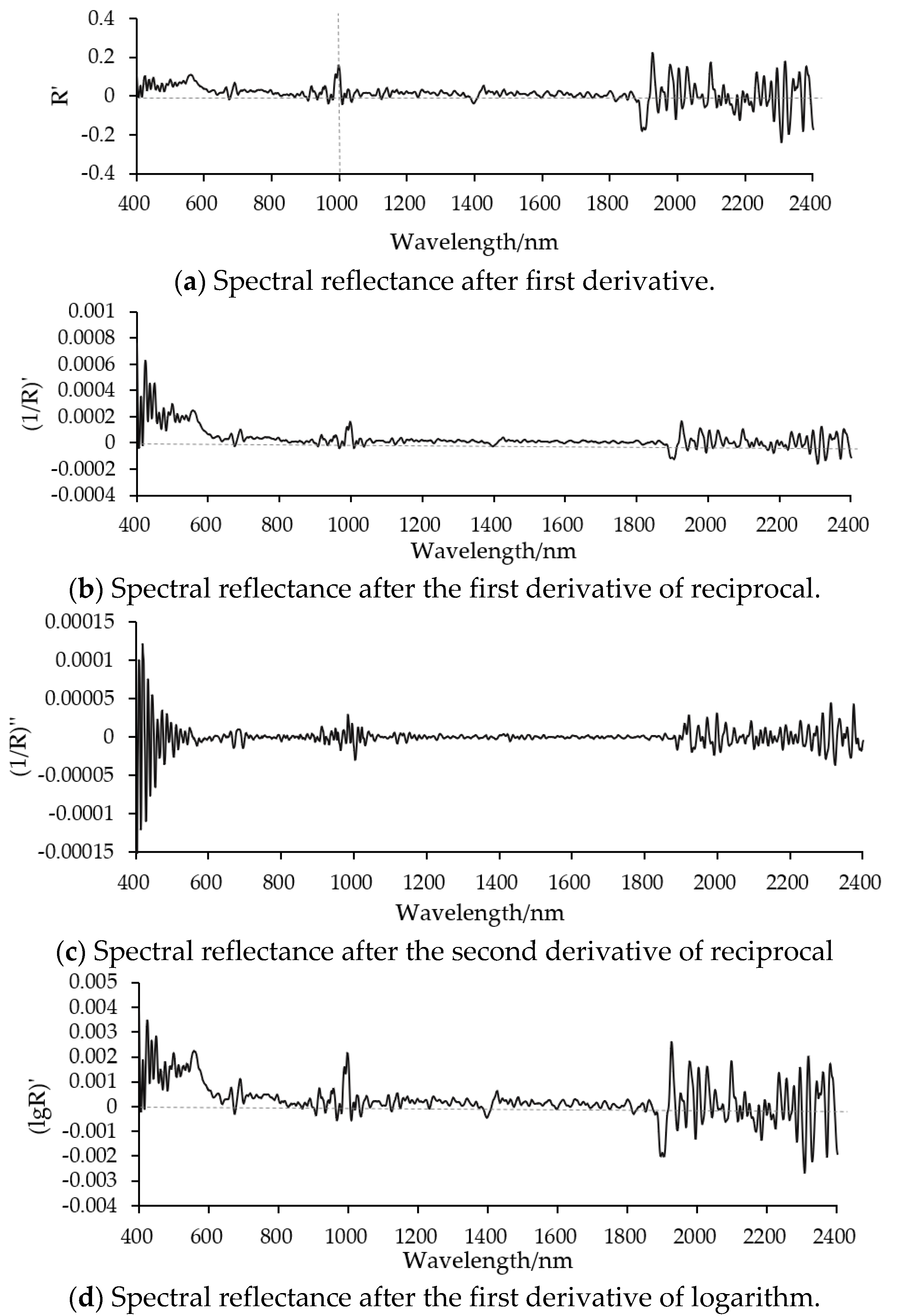
3.1. Spectral Characteristics of Coastal Wetland Soil

As can be seen from Table 1, the SOM content of the 34 samples collected is between 7 and 45.3 mg.kg−1, the TN content is between 0.24 and 2.08 mg.kg−1, and the TC content is between 4.2 and 34 mg.kg−1. The standard deviation and coefficient of variation of the SOM content are the largest, which indicates that the SOM content in each sample soil collected is highly dispersed and unevenly distributed.
We choose 400–2400 nm for analysis because there are many noises in the original spectra between 350 and 400 nm. In MATLAB2014b, Savitzky–Golay (S–G) filter is applied to being smoothened the original spectra of the soil in the coastal wetland by five-order polynomial filter to improve the smoothness of the spectra and reduce the noise interference. The indoor reflectance spectral curves of the topsoil samples (Figure 2) range from 0.1 to 0.7 in the total band. It can be clearly found that the soil spectral curve has two distinct absorption valleys near the two bands of 1400–1900 nm, and there are two weak absorption valleys near the 700 nm and 1000 nm bands in virtue of water molecules in the soil sample vibration frequency generated with the frequency combiner. In the 1950–2400 nm spectra, the spectra are in a wave form, mainly because of the small amount of moisture in the soil samples and the moisture absorption in the air. On the whole, the reflectance spectra curves of the soil present a parabolic pattern, and its reflectance increases with the increase of the wavelength. Among them, the rising speed is obvious in the range of 400–600 nm, and it is moderately slow in the range of 600–800 nm. After 800 nm, the rise of the spectral reflectance is relatively gentle.

3.2. Extraction of Characteristic Bands of SOM, TN, and TC Contents in Soil

The spectral reflectance after S–G filtering is transformed into the first derivative transformation (Figure 3a), first derivative of reciprocal transformation (Figure 3b), second derivative of reciprocal transformation (Figure 3c), and first derivative of logarithmic transformation (Figure 3d). For convenience, the reflectance spectrum curve of the No.3 sampling soil is randomly selected for observation.
The band of no.3 soil sample is mainly positive between 400 and 1800 nm after the R′, (1/R), (lgR)′ differential transformation. It fluctuates between the band of 1800–2400 nm in a large range of positive and negative fluctuation, and there are more peaks and troughs. (1/R)″ differential transformation amplifies the reflectance rising band of 400–600 nm of the original spectral curve, and multiple peaks appear. After the differential transformation of (1/R)′ and the (lgR)′ differential transformation, the weak absorption valleys of 700–1000 nm of the original spectral curve were amplified, and more peak bands appeared. It can be found that the differential transformation can amplify the subtle changes in the original spectral curve, which is convenient for further extracting the characteristic bands corresponding to the SOM, TN, and TC elements in the soil.
Correlation analysis between the SOM, TN, and TC contents of the 34 topsoil samples and the transformed forms of reflectance spectra was carried out in detail. Finally, the wavelength of the significant level p < 0.01 was selected as the characteristic band (Table 2).
Viewed from Table 2, it is indicated that the number of characteristic bands extracted from each differential transformation is not the same. The correlation coefficients between SOM, TN, and TC contents in soil and the differential transformation are also different. The spectral transformation of (1/R)′ has the best correlation with the SOM content in soil. There are 13 characteristic bands, which are respectively 498–501 nm, 1180–1182 nm, 1946 nm, 1947 nm, and 2323–2326 nm. Among them, there is a positive correlation near the 2324 nm and a negative correlation near the 500 nm band. For the highest correlation between the soil TN content and (1/R)′ there are 14 characteristic bands, which are 536 nm, 900 nm, 1177 nm, 1178 nm, 1285–1287 nm, 1977 nm, 2319 nm–2322 nm, 2345 nm, and 2346 nm respectively. It is positively correlated at 2320 nm and negatively correlated at 1170 nm. For the highest correlation between the soil TC content and (1/R)′ there are 24 characteristic bands: 536–537 nm, 561–562 nm, 619–622 nm, 899–900 nm, 1234–1235nm, 1438–1439 nm, 1795–1796 nm, 1949–1952 nm, 2345–2347 nm, and 2373 nm, in which the positive correlation is presented in the vicinity of the 2346 nm and negative correlation is presented in the vicinity of the 1951 nm band.

3.3. Model Construction and Accuracy Verification

3.3.1. Hyperspectral Estimation Model of SOM, TN, and TC Content Based on SVM

The total 34 topsoil samples were divided into two groups (24 for the training set, the remaining 10 for the test set). The characteristic band data of 24 soil samples and the corresponding soil SOM, TN, and TC contents were selected as the input and output of the training set respectively. The variables for the input and output of the test set were the characteristic band data of 10 soil samples and the corresponding soil SOM, TN, and TC contents respectively. For example, for the SOM of soil samples based on the (1/R)′, the randomly selected 24 samples and the extracted 13 characteristic band data constituted a 24 × 13 doubt type matrix as the input of the SVM training set. The corresponding soil organic matter content was composed of 24 × 1 doubt type matrix as the output of the training set. The remaining 10 samples and the data of the 13 characteristic bands constituted a 10 × 13 doubt matrix as the input of the test set, while the 10 samples corresponding to the measured SOM content constituted a 10 × 1 doubt matrix as the output of the test set.
Since the input data units were different and some data ranges were relatively large, this would lead to a too long training time, and the input of different ranges would also affect the accuracy of the modeling. Therefore, the data of training set and test set were normalized by using the “mapminmax” function in MATLAB2014b, and then mapped to [0, 1] interval. Its normalization algorithm is as follows:
y = x min max min
In the formula, the min is the minimum value and the max is the maximum value in the input sample set. In the creation and training of the SVM, the type of “−t” kernel function was chosen as the RBF kernel function. The method of using the grid search cross-validation traversal c and g values that obtained the optimum parameters of the c and g, “−s” namely the SVM type selection for e-SVR type and “−p” set the value of the loss function p in the e-SVR type as 0.01. Finally, the “Svmpredict“ function and the trained model are used to predict the effective values of the remaining 10 samples, and the predicted values are reversely normalized using “mapminmax” function to better restore the real values. The final model validation accuracy is shown in Table 3.
Table 3 shows that the first-order differential of reciprocal reflectance of soil samples has the highest accuracy in estimating SOM contents, the predictive determination coefficient R2 is 0.93, and the predictive root mean square error (RMSE) is 0.23. The second-order differential of reciprocal reflectance of soil samples has the highest accuracy in estimating soil TN content, the R2 is 0.88 and RMSE is 0.17. The second order differential estimated soil TC content with the highest accuracy is also the highest, the R2 is 0.85 and RMSE is 0.26.

3.3.2. Hyperspectral Estimation Model of SOM, TN and TC contents Based on BP Neural Network

The modeling form of the BP neural network is similar to the SVM model. Both training sets and test sets need to be set in order to facilitate the observation and the accuracy comparison of the two models. The same test set and training set as the SVM modeling are selected. At the same time, similar to SVM modeling, both the training set and the test set must be normalized to map them to the [0, 1] interval. When creating a neural network, the training method selects the gradient descent method, the number of iterations is set to 1000 times, the training target is set to e−30, that is, the RMSE of the training is less than le-30, the number of neurons is set to 10, and the learning rate is set to 0.01. After the simulation test is the same as the de-normalization and SVM modeling. The final model precision is shown in Table 4.
Table 4 shows that the precision of estimating the SOM content by the first-order differential of reciprocal reflectance of soil samples is higher, the predictive determinant coefficient R2 is 0.87, and the prediction RMSE is 0.33. The precision of estimating the soil TN content by the second-order differential of reciprocal reflectance of soil samples is higher, the R2 is 0.79, and the RMSE is 0.46. At the same time, the precision of estimating the TC content by the second-order differential of reciprocal reflectance of soil samples is higher, the R2 is 0.79, and the RMSE is 0.38.

3.3.3. Accuracy Comparison between SVM and BP for Detecting Soil SOM, TN and TC

Figure 4 shows the comparison between the accuracy of SVM and the BP neural network in the estimation of the soil nutrient content in coastal wetlands. Figure 4a shows the estimation accuracy of the SOM content. Figure 4b shows the estimation accuracy of the TN content. Figure 4c shows the estimation accuracy of the TC content. The abscissa represents four different forms of spectral transformation, the left ordinate represents the value of the determination coefficient R2, and the right ordinate represents the value of RMSE.
Viewed from Figure 4, it was indicated that, based on the coefficient of determination R2 and RMSE evaluation indicators, the accuracy of estimating the SOM and TN content in coastal wetlands by SVM is better than that of the BP neural network. In order to more intuitively evaluate the prediction effect of the SVM model, the soil SOM content in the coastal wetland predicted by the SVM model constructed by spectral transformation (1/R)′ is compared with the measured SOM content (Figure 5a). The abscissa coordinate was the measured value and the longitudinal coordinate was the predicted value. Figure 5b shows the comparison of the TN content predicted by the SVM model using spectral transformation (1/R)″ with the measured TN content. Figure 5c is the comparison of the TC content predicted by the SVM model using spectral transformation (1/R)″ with the measured TC content. It can be seen from Figure 5 that SVM has a high accuracy in predicting SOM, TN, and TC, which are uniformly distributed near the line y = x.

4. Discussion

4.1. The Characteristics of Reflectance Spectra for Soils in Coastal Wetland

It can be seen from Figure 2 that the spectral curves for the 34 naturally-dried soil samples have great similarities. However, due to the different SOM, TN, and TC content in each soil sample, the measured spectral reflectance of soil samples is also different in wave peaks, troughs, and reflectance strength, which is the same as the results of Cécile et al. [44]. The spectral reflectance of the third core area of Dafeng Elk National Nature Reserve ranges from 0.1 to 0.7. The spectral reflectance curve is steep near the 400–800 nm, while the reflectance curve of the 800–2400 nm tends to be gentle. There are two obvious absorption valleys around 1400nm and 1900nm, which is consistent with the results of most scholars who study the spectral reflectance characteristics of soil [6,7,8,9]. Previous studies have shown that increasing the SOM content in soil will reduce the spectral reflectance of the soil [45]. However, the results of this study showed (Figure 6) that soil sample No. 34 with the highest SOM content (45.3 mg.kg−1) had higher spectral reflectance than the soil sample No. 23 with the lowest SOM content (7 mg.kg−1). It may be due to the fact that the subtypes of tidal saline soil and meadow coastal saline soil in the third core area of Dafeng Elk National Nature Reserve are greatly affected by ocean tides, and the salt content is relatively high, thus reducing the spectral reflectance of the SOM content in the soil. Until now, researchers have discovered that the spectral reflectance of SOM in the coastal wetland soil is significantly higher than that of the non-wetland soils. For example, Gao et al. [15] found that the SOM content in Minjiang Estuary wetland soil was directly proportional to the spectral reflectance in the band of 600–2500 nm. Wang et al. [46] found that the increasing soil salinity in the Yellow River delta wetland would also result in a higher spectral reflectance.

4.2. The Sensitive Bands and Estimation Accuracy for SOM, TN and TC Contents of Coastal Wetland Soil

After S–G filtering and (1/R)′ transformation, the original spectral reflectance has a high and negative correlation with the SOM content in soil around 500 nm. The sensitive bands extracted were 498–501 nm, 1180–1182 nm, 1946 nm, 1947 nm and 2323–2326 nm. After (1/R)″ transformation, it is highly correlated with the soil TN and TC contents. The TN sensitive bands are 536 nm, 900 nm, 1177 nm, 1178 nm, 1285–1287 nm, 1977 nm, 2319–2322 nm, 2345 nm and 2346 nm. The TC sensitivity bands are 536–537 nm, 561–562 nm, 619–622 nm, 899–900 nm, 1234–1235 nm, 1438–1439 nm, 1795–1796 nm, 1949–1952 nm, 2345–2347 nm, and 2373 nm. These bands are different from the SOM sensitive bands: 362 nm, 392 nm, 422 nm, 437 nm, 537 nm, 652 nm, 702 nm and 1062 nm extracted by continuous projection method of the collected paddy soil, brick laterite, and loess by Zhang et al. [35]. This is also different from the TN sensitive bands of 500–900 nm and 1350–1490 nm extracted by the Norris filter and the first-order differential transformation of soil collected by Zhang et al. [47] in the middle and eastern China. However, the soils of the Sanjiangyuan region of China collected by Yang [48], using differential transformation, are similar to the TC sensitivity bands of 500–900 nm, 1400–1500 nm, 1900–2000 nm, and 2200–2300 nm. The reason for the difference in the above research results may be the different soil types in the study area. The soil types in the third core area of Dafeng Elk National Nature Reserve are mainly tidal flat salt soil and meadow coastal salt soil. These two soil types usually contain between 0.8 and 2.0% salt, and the highest salt content is as much as 4% [49]. The spectra reflectance of the soil and the spectral information of SOM, TN, and TC in soil will be further affected by the soil salinity [15].
The results of this study indicate that the accuracy of SOM, TN, and TC in soil by SVM is better than that of the BP neural network, which is consistent with the results of the estimation model of nitrogen, phosphorus, and potassium in Zhangzhou red soil and Haining green purple mud constructed by Jiang et al. [50] through least squares support vector machine and BP neural network. In this study, the SVM estimation model constructed by the (1/R)′ transformation of the spectrum has the highest accuracy in predicting the SOM content of the coastal wetland soil, R2 is 0.93 and the RMSE is 0.23. It is higher than the accuracy (R2 = 0.84) of the SOM content in Jianghan Plain predicted by Yu et al. [33] by partial least squares regression modeling method. At the same time, it is better than the prediction accuracy (R2 = 0.83) of the SOM content in Meijiang Township, Suichuan County, Jiangxi Province constructed by Liu [51] with first-order differential and least squares regression method. In this study, the SVM estimation model of the TN and TC content in coastal wetland soil constructed by the (1/R)″ transformation of the spectrum, the prediction coefficient R2 is 0.88 and 0.85 respectively, RMSE is 0.17 and 0.26 respectively. This is better than the prediction accuracy (R2 = 0.832) of the TN content of the Minjiang Estuary wetland constructed by exponential transformation and unary linear regression by Gao et al. [15], and is also superior to Yang [48] in predicting the TC content of marsh soil in the Sanjiangyuan region of China by BP neural network (R2 = 0.81). This indicates that the SVM model based on the differential transformation form of hyperspectral reflectance has certain feasibility in predicting SOM, TN, and TC content in coastal wetlands soil, but whether the model can predict the nutrient content in the coastal wetland soil in other areas needs further verification.
Viewed from the number of soil samples, although the number of samples in this experiment is only 34, the estimation accuracy of the soil TN content by using the SVM model is higher than that of the 140 surface soil samples collected by Antonions et al [52]. In addition to the differences in the study area, another important reason may be the difference in the number of sampling points and the sampling interval. Therefore, in the future, the effect of the sampling interval of sample points and the number of samples on the model accuracy should be discussed in depth.

5. Conclusions

In this study, 34 topsoil samples were collected in the coastal wetland and reflectance spectra of soil samples were measured in a dark room. All of the reflectance spectra were preprocessed by S–G filtering and then subjected to four differential transformations of R′, (1/R)′, (1/R)″, and (lgR)′ respectively. Next, the correlation coefficient was analyzed in order to retrieve the characteristic bands which were sensitive to soil SOM, TN, and TC contents. The estimation models of soil SOM, TN, and TC contents in coastal wetland soil were determined based on support vector machine (SVM) and BP neural network algorithms. The major findings are as follows:
(1)
The model accuracy based on SVM in detecting soil SOM, TN and TC contents is significantly better than that based on the BP neural network.
(2)
There is a high correlation between SOM and the reciprocal (1/R)′ of reflectance spectra, the number of bands with significant correlation (p < 0.01) were 13 and the correlation is the highest at 500 nm, the correlation coefficient (R) is −0.484. There is a relative high correlation between TN and the second-order differentials (1/R)″ of reflectance spectra. The number of bands with significant correlation (p < 0.01) was 14, and the highest correlation at 2320 nm is found with correlation coefficient (R) of 0.574. There is also a high correlation between TC and the second-order differentials (1/R)″ of reflectance spectra. There are 24 bands, which are significantly correlated (p < 0.01), and the highest correlation at 2346 nm is determined with the correlation coefficient (R) of 0.579.
(3)
The accuracy of the estimation model of SOM based on SVM is the highest, with the prediction coefficient R2 of 0.93 and RMSE of 0.23 mg kg−1, respectively.
(4)
In the future, the impact of the numbers of soil samples on the accuracy of the estimation model and root mean square error should be further discussed.

Author Contributions

X.L. and S.Z. conceived and designed the experiment; S.Z. performed the experiments and analyzed the data; Y.Z. improved the data analysis and supervised the research; S.Z., G.N., and Y.L. drafted the paper; Y.Z. edited the paper.

Funding

This research was jointly supported by the National Natural Science Foundation of China (No. 41506106), the Key Laboratory for Geo-Environmental Monitoring of Coastal Zone of the National Administration of Surveying, Mapping and Geo-information (No. GE-2017-003), the Marine Technology Brand Specialty Construction Project of Jiangsu Province (No. PPZY2015B116), the Pioneer Science and Technology Special Training Program B (No. XDPB11-01-04) of Chinese Academy of Sciences, and the China-Italy Collaborate Project for Lunar Surface Mapping (No. 2016YFE0104400).

Conflicts of Interest

The authors declare no conflict of interests.

References

  1. Nadi, M.; Golchin, A.; Sedaghati, E.; Shafie, S.; Hosseini fard, S.J.; Füleky, G. Using Nuclear Magnetic Resonance 1H and 13C in soil organic matter covered by forest. J. Soil Water Conserv. 2017, 21, 83–92. [Google Scholar] [CrossRef] [Green Version]
  2. Ma, K.; Zhang, Y.; Tang, S.X.; Liu, G. Characteristics of spatial distribution of soil total nitrogen in Zoigen alpine wetland. Chin. J. Ecol. 2016, 35, 1988–1995. [Google Scholar]
  3. Jauss, V.; Sullivan, P.; Lehmann, J.; Sanderman, J.; Daub, M. Alternative modelling approaches for estimating pyrogenic carbon, soil organic carbon and total nitrogen in contrasting ecoregions within the United States. Geophys. Res. Abstr. 2017, 19, 497. [Google Scholar]
  4. Lu, X.; Lin, Y.L.; Wu, Y.N.; Gu, Y.; Zhao, Q.; Zhang, X. Spatial Distribution Characteristics of Soil Physical and Chemical Properties in Milu National Nature Reserve of Coastal Wetland. Trans. Oceanol. Limnol. 2018, 4, 74–81. [Google Scholar]
  5. Vohland, M.; Emmerling, C. Determination of total soil organic C and hot water-extractable C from VIS-NIR soil reflectance with partial least squares regression and spectral feature selection techniques. Soil Sci. 2011, 62, 598–606. [Google Scholar] [CrossRef]
  6. Wu, D.; Shi, H.; Wang, S.J.; He, Y.; Bao, Y.D.; Liu, K.S. Rapid prediction of moisture content of dehydrated prawns using online hyperspectral imaging system. Anal. Chim. Acta 2012, 726, 57–66. [Google Scholar] [CrossRef] [PubMed]
  7. Wu, G.F.; He, Y. Application of Wavelet Threshold Denoising Model to Infrared Spectral Signal Processing. Spectrosc. Spectr. Anal. 2009, 29, 3246–3249. [Google Scholar]
  8. Radim, V.; Radka, K.; Aleš, K.; Luboš, B. Simple but efficient signal pre-processing in soil organic carbon spectroscopic estimation. Geoderma 2017, 298, 46–53. [Google Scholar]
  9. Shen, Y.; Zhang, X.P.; Liang, A.Z.; Shi, X.H.; Fan, R.Q.; Yang, X.M. Multiplicative scatter correction and step is regression to build NIRS model for analysis of soil Organic Carbon content in black soil. Syst. Sci. Compr. Stud. Agric. 2010, 26, 174–180. [Google Scholar]
  10. Hu, T.; Qi, K.; Hu, Y. Using vis-nir spectroscopy to estimate soil organic content. In Proceedings of the IGARSS 2018—2018 IEEE International Geoscience and Remote Sensing Symposium, Valencia, Spain, 22–27 July 2018. [Google Scholar]
  11. Chen, H.Y. Hyperspectral Estimation of Major Soil Nutrient Content. Ph.D. Thesis, Shandong Agricultural University, Shandong, China, 2012. [Google Scholar]
  12. Sun, W.; Li, X.; Niu, B. Prediction of soil organic carbon in a coal mining area by Vis-NIR spectroscopy. PLoS ONE 2018, 13. [Google Scholar] [CrossRef]
  13. Chen, H.Y.; Zhao, G.X.; Li, X.C.; Zhu, X.C.; Sui, L.; Wang, Y.J. Hyperspectral estimation of soil organic matter content based on wavelet transformation. Chin. J. Appl. Ecol. 2011, 22, 2935–2942. [Google Scholar]
  14. Sorenson, P.T.; Small, C.; Tappert, M.C.; Quideau, S.A.; Drozdowski, B.; Underwood, A.; Janzd, A. Monitoring organic carbon, total nitrogen, and pH for reclaimed soils using field reflectance spectroscopy. Can. J. Soil Sci. 2017, 97, 241–248. [Google Scholar] [CrossRef] [Green Version]
  15. Gao, D.Z.; Zeng, C.S.; Zhang, W.L.; Liu, Q.Q.; Wang, Z.P.; Chen, Y.T. Estimating of soil total nitrogen concentration based on hyperspectral remote sensing data in Minjiang River estuarine wetland. Chin. J. Ecol. 2016, 35, 952–959. [Google Scholar]
  16. Wu, M.Z.; Li, X.M.; Sha, J.M. Spectral Inversion Model for Prediction of Red Soil Total Nitrogen Content in Subtropical Region (Fuzhou). Spectrosc. Spectr. Anal. 2013, 33, 3111–3115. [Google Scholar]
  17. He, Y.; Xiao, S.; Nie, P.; Dong, T.; Qu, F.; Lin, L. Research on the Optimum Water Content of Detecting Soil Nitrogen Using Near Infrared Sensor. Sensors 2017, 17, 2045. [Google Scholar] [CrossRef]
  18. Zhou, X.B.; Zhao, J.W. Methods of Characteristic Wavelength Region and Wavelength Selection Based on Genetic Algorithm. Acta Opt. Sin. 2007, 27, 1316–1321. [Google Scholar]
  19. Zhang, Y. Research on Spectral Region Selection of Near Infrared Spectra Based on Genetic Algorithm. In Proceedings of the 2017 9th International Conference on Intelligent Human-Machine Systems and Cybernetics (IHMSC), Hangzhou, China, 26–27 August 2017. [Google Scholar]
  20. Krishnan, P.; Alexander, J.D.; Butler, B.J.; Hummel, J.W. Reflectance Technique for Predicting Soil Organic Matter. Soil Sci. Soc. Am. J. 1980, 44, 1282–1285. [Google Scholar] [CrossRef]
  21. Tahmasbian, I.; Xu, Z.; Abdullah, K.; Zhou, J.; Esmaeilani, R.; Nguyen, T.T.N.; Bai, S.H. The potential of hyperspectral images and partial least square regression for predicting total carbon, total nitrogen and their isotope composition in forest litterfall samples. J. Soil Sediment. 2017, 17, 2019–2103. [Google Scholar] [CrossRef]
  22. Couteaux, M.; Berg, B.; Rovira, P. Near infrared reflectance spectroscopy for determination of organic matter fractions including microbial biomass in coniferous forest soils. Soil Biol. Biochem. 2003, 35, 1587–1600. [Google Scholar] [CrossRef]
  23. Vanwaes, C.; Mestdagh, I.; Lootens, P.; Caflier, L. Possibilities of near infrared reflectance spectroscopy for the prediction of organic carbon concentrations in grassland soils. J. Agric. Sci. 2005, 143, 487–492. [Google Scholar] [CrossRef]
  24. Heike, G.; Gunter, M.; Hermann, K. Spatially explicit estimation of clay and organic carbon content in agricultural soils using multi-annual imaging spectroscopy data. Appl. Environ. Soil Sci. 2012, 2012, 868090. [Google Scholar]
  25. Mouazen, A.M.; Maleki, M.R.; Cockx, L.; Meirvenne, M.V.; Holme, L.H.J.V.; Merckx, R.; Baerdemaeker, J.D.; Ramon, H. Optimum three-point linkage set up for improving the quality of soil spectra and the accuracy of soil phosphorus measured using an on-line visible and near infrared sensor. Geoderma 2009, 103, 144–152. [Google Scholar] [CrossRef] [Green Version]
  26. Jiang, Q.; Li, Q.; Wang, X.; Wu, Y.; Yang, X.; Liu, F. Estimation of soil organic carbon and total nitrogen in different soil layers using VNIR spectroscopy: Effects of spiking on model applicability. Geoderma 2017, 293, 54–63. [Google Scholar] [CrossRef]
  27. Tian, Y.C.; Zhang, J.J.; Yao, X.; Cao, W.X.; Zhu, Y. Laboratory assessment of three quantitative methods for estimating the organic matter content of soils in China based on visible/near-infrared reflectance spectra. Geoderma 2013, 202–203, 161–170. [Google Scholar] [CrossRef]
  28. Tang, R.; Chen, K.; Jiang, C.; Li, C. Determining the Content of Nitrogen in Rubber Trees by the Method of NIR Spectroscopy. J. Appl. Spectrosc. 2017, 84, 627–632. [Google Scholar] [CrossRef]
  29. Liu, X.M.; Liu, J.S. Based on the LS-SVM Modeling Method Determination of Soil Available N and Available K by Using Near Infrared Spectroscopy. Spectrosc. Spectr. Anal. 2012, 32, 3019–3023. [Google Scholar]
  30. Kennedy, W.; Dieu, T.B.; Øystein, B.D.; Bal, R.S. A comparative assessment of support vector regression, artificial neural networks, and random forests for predicting and mapping soil organic carbon stocks across an Afromontane landscape. Ecol. Indic. 2015, 52, 394–403. [Google Scholar]
  31. Dalal, R.C.; Henry, R.J. Simultaneous determination of moisture, organic carbon, and total nitrogen by near infrared reflectance spectroscope. Soil Sci. Soc. Am. J. 1986, 50, 120–123. [Google Scholar] [CrossRef]
  32. Zhang, J.J. Estimating Soil Nutrient Information Based on Spectral Analysis Technology. Ph.D. Thesis, Nanjing Agricultural University, Nanjing, China, 2009. [Google Scholar]
  33. Yu, L.; Hong, Y.S.; Geng, L.; Zhou, Y.; Zhu, Q.; Cao, J.J.; Nie, Y. Hyperspectral estimation of soil organic matter content based on partial least squares regression. Trans. Chin. Soc. Agric. Eng. 2015, 31, 103–109. [Google Scholar]
  34. Bao, N.S.; Wu, L.X.; Ye, B.Y.; Yang, K.; Zhou, W. Assessing soil organic matter of reclaimed soil from a large surface coal mine using a field spectroradiometer in laboratory. Geoderma 2017, 288, 47–55. [Google Scholar] [CrossRef]
  35. Zhang, H.L.; Liu, X.M.; He, Y. Measurement of Soil Organic Matter and Available K Based on SPA-LS-SVM. Spectrosc. Spectr. Anal. 2014, 34, 1348–1351. [Google Scholar]
  36. Huete, A.R. Estimation of soil properties using hyperspectral VIS/IR sensors. Encycl. Hydrol. Sci. 2006, 15, 887–901. [Google Scholar]
  37. Kooistra, L.; Salas, E.A.L.; Clevers, J.G.P.W.; Wehrens, R.; Leuven, R.S.E.W.; Nienhuis, P.H.; Buydens, L.M.C. Exploring field vegetation reflectance as an indicator of soil contamination in river floodplains. Environ. Pollut. 2004, 127, 281–290. [Google Scholar] [CrossRef]
  38. Wang, X.P.; Zhang, F.; Kung, H.; Verner, C.J. New methods for improving the remote sensing estimation of soil organic matter content (SOMC) in the Ebinur Lake Wetland National Nature Reserve (ELWNNR) in northwest China. Remote Sens. Environ. 2018, 218, 104–118. [Google Scholar] [CrossRef]
  39. Liu, J.G.; Xue, J.H.; Wang, L.; Ding, J.J.; Wang, W.L.; Liu, C.G.; Rong, Y. Habitat degradation features of Pere David’s Deer Natural Reserve in Dafeng of Jiangsu Province, East China. Chin. J. Ecol. 2011, 30, 1793–1798. [Google Scholar]
  40. Ye, Z.G. Research on Nutrient Evolution in BoZhou Tillage. Master’s Thesis, Anhui Agricultural University, Hefei, China, 2007. [Google Scholar]
  41. Li, G.H.; Ye, X.L.; Yang, S.; Wen, Y.J.; Huang, J.S.; Liu, Y.X.; Wang, H. Comparison of total soil carbon determination by catalytic oxidation method and direct combustion method. Soil Fertil. Sci. China 2014, 4, 97–101. [Google Scholar]
  42. Zhang, Q.; Zhang, G.L.; Zhang, Z.; Lv, X. Predicting of Soil Total Nitrogen Content Based on Hyperspectral Data. J. Shanxi Agric. Sci. 2016, 44, 972–976. [Google Scholar]
  43. Tian, Y.; Shen, R.P.; Ding, G.X. Application of Support Vector Machine on Soil Magnesium Content Estimation Based on Hyper-Spectra. Soils 2015, 47, 602–607. [Google Scholar]
  44. Cécile, G.; Raphael, A.; Viscarra, R.; Alex, B.M.B. Soil organic carbon prediction by hyperspectral remote sensing and field vis-NIR spectroscopy: An Australian case study. Geoderma 2008, 146, 403–411. [Google Scholar]
  45. Li, Y.M.; Wang, Q.; Huang, J.Z. Ground Remote Sensing Experiment Principles and Methods; Science Press: Beijing, China, 2011. [Google Scholar]
  46. Wang, L.; Zhu, X.C.; Liu, Q.; Zhao, G.X.; Liu, H.Y.; Wang, L.; Zhang, S.W. Hypersperpectral Quantitative Estimation of Saline-alkali Soil Salinity in the Yellow River Delta. Chin. J. Soil Sci. 2013, 44, 1101–1106. [Google Scholar]
  47. Zhang, J.J.; Tian, Y.C.; Yao, X.; Cao, W.X.; Ma, X.M.; Zhu, Y. Estimating Soil Total Nitrogen Content Based on Hyperspectral Analysis Technology. J. Natl. Resour. 2011, 26, 881–890. [Google Scholar]
  48. Yang, Y. Hyperspectral Inversion of Soil Total Nitrogen, Total Carbon and Carbon-Oxygen Ratio in Sanjiangyuan District. Master’s Thesis, Qinghai University, Qinghai, China, 2014. [Google Scholar]
  49. Zhang, X.Q. Discussion on the Evolution of Coastal Wetland and the Construction Mode of Nature Reserve in Yancheng, Jiangsu Province; Shandong People’s Publishing House: Jinan, China, 2013; p. 35. [Google Scholar]
  50. Jiang, L.L.; Zhang, Y.; Wang, Y.Y.; Tan, L.H.; He, Y. Fast determination of nutritional parameters in soil based on spectroscopic techniques. J. Zhejiang Univ. 2010, 36, 445–450. [Google Scholar]
  51. Liu, X.M. Near infrared diffuse reflectance spectra detection of soil organic matter and available N. J. Chin. Agric. Mech. 2013, 34, 202–206. [Google Scholar]
  52. Antonios, M.; Xanthoula, E.P.; Dimitrios, M.; Thomas, A.; Rebecca, W.; Georgios, T.; Jens, W.; Ralf, B.; Abdul, M.M. Machine learning based prediction of soil total nitrogen, organic carbon and moisture content by using VIS-NIR spectroscopy. Biosyst. Eng. 2016, 152, 104–116. [Google Scholar]
Figure 1. The spatial distribution of soil samples in the study area.
Sustainability 11 00667 g001
Figure 2. Soil sample reflectance curve after Savitzky–Golay (S–G) filtering.
Sustainability 11 00667 g002
Figure 3. Spectral reflectance curve after differential transformation.
Sustainability 11 00667 g003
Figure 4. Comparison of modeling accuracy of soil organic matter (SOM), total nitrogen (TN), and total carbon (TC) content.
Sustainability 11 00667 g004
Figure 5. The prediction of soil SOM, TN, and TC content.
Sustainability 11 00667 g005
Figure 6. The spectral reflectance of soil samples No. 23 and No. 34.
Sustainability 11 00667 g006
Table 1. The statistical results of soil samples in the study area.
PropertyMinMaxSDMeanCV
SOM (mg kg−1)745.38.313.263.1
TN (mg kg−1)0.242.080.40.755.8
TC (mg kg−1)4.234.87.01450.8
Min: minimum; Max: maximum; SD: standard deviation; CV: coefficient of variation.
Table 2. Sensitive band deletion of soil organic matter (SOM), total nitrogen (TN), and total carbon (TC) content.
ElementsTransformationMaximum CorrelationMinimum CorrelationNumberSensitive Band nm (p < 0.01)
Band nmRBand nmR
SOMR′8550.468 **2213−0.402 *2855, 854
(1/R)′23240.479 **500−0.484 **13498–501, 1180–1182, 1946, 1947, 2323–2326
(lgR)′8550.441 **534−0.465 **3533, 534, 855
(1/R)″9000.477 **1952−0.425 *7874, 899, 900, 901, 2319, 2320, 2346
TNR′12910.543 **1358−0.442 *21514, 515, 785–790, 854–856, 1290–1293, 1358, 1359, 1493–1496
(1/R)′23250.547 **500−0.558 **46496–502, 523–525, 530–534, 1179–1184, 1239–1243, 1268, 1291, 1292, 1358–1360, 1426–1428, 1947, 1948, 2323–2327, 2339–2342
(1/R)″23200.574 **1177−0.472 **14536, 900, 1177, 1178, 1285–1287, 1977, 2319–2322, 2345, 2346
(lgR)′12910.502 **1359−0.458 **25786–789, 855, 856, 1181, 1182, 1241, 1242, 1290–1293, 1358–1360, 1494, 1947, 1948, 2324–2326, 2340, 2341
TCR′19460.538 **2368−0.474 **42479, 480, 642–644, 689–691, 726–732, 785–791, 990–996, 1798–1801, 1943–1948, 2367–2369
(1/R)′19460.569 **1240−0.521 **49494–501, 531–534, 638–644, 696, 697, 1179–1184, 1238–1244, 1799, 1800, 1801, 1930, 1931, 1943–1948, 2340–2342, 2367
(1/R)″23460.579 **1951−0.538 **24536, 537, 561, 562, 619–622, 899, 900, 1234, 1235, 1438, 1439, 1795, 1796, 1949–1952, 2345–2347, 2373
(lgR)′19450.559 **1240−0.488 **37479, 480, 639–644, 696, 697, 728, 785–791, 993, 994, 1239–1242, 1358, 1798–1801, 1943–1948, 2367, 2368
** and *, is significant at the level 0.01 and 0.05%, respectively.
Table 3. Results of soil SOM, TN and TC contents obtained by support vector machine (SVM).
ElementsVariableEstimation modelValidation Model
R2RMSER2RMSE
SOMR′0.74 **0.390.72 **0.7
(1/R)′0.68 **0.280.93 **0.23
(lgR)′0.89 **0.180.7 **0.34
(1/R)″0.84 **0.320.84 **0.24
TNR′0.74 **0.370.67 **0.26
(1/R)′0.63 **0.310.61 **0.65
(lgR)′0.76 **0.240.71 **0.19
(1/R)″0.87 **0.27>0.88 **0.17
TCR′0.64 **0.310.7 **0.18
(1/R)′0.57 **0.40.54 *0.29
(lgR)′0.82 **0.220.63 **0.38
(1/R)″0.86 **0.230.85 **0.26
** and *, is significant at the level 0.01 and 0.05%, respectively.
Table 4. Result of soil SOM, TN and TC contents obtained by back propagation (BP).
ElementsVariableEstimation modelValidation Model
R2RMSER2RMSE
SOMR′0.89 **0.260.7 **0.24
(1/R)′0.83 **0.090.87 **0.33
(lgR)′0.95 **0.020.63 **0.44
(1/R)″0.66 *0.060.77 **0.18
>TNR′0.85 **0.080.52 *0.54
(1/R)′0.82 **0.090.53 *0.6
(lgR)′0.82 **0.040.69 **0.35
(1/R)″0.85 **0.050.79 **0.46
TCR′0.86 **0.130.62 **0.48
(1/R)′0.93 **0.030.43 *0.52
(lgR)′0.9 **0.040.6 **0.33
(1/R)″0.6 *0.190.79 **0.38
** and *, is significant at the level 0.01 and 0.05%, respectively.

