A Statistical Approach for Studying the Spatio-Temporal Distribution of Geolocated Tweets in Urban Environments

Abstract

An in-depth descriptive approach to the dynamics of the urban population is fundamental as a first step towards promoting effective planning and designing processes in cities. Understanding the behavioral aspects of human activities can contribute to their effective management and control. We present a framework, based on statistical methods, for studying the spatio-temporal distribution of geolocated tweets as a proxy for where and when people carry out their activities. We have evaluated our proposal by analyzing the distribution of collected geolocated tweets over a two-week period in the summer of 2017 in Lisbon, London, and Manhattan. Our proposal considers a negative binomial regression analysis for the time series of counts of tweets as a first step. We further estimate a functional principal component analysis of second-order summary statistics of the hourly spatial point patterns formed by the locations of the tweets. Finally, we find groups of hours with a similar spatial arrangement of places where humans develop their activities through hierarchical clustering over the principal scores. Social media events are found to show strong temporal trends such as seasonal variation due to the hour of the day and the day of the week in addition to autoregressive schemas. We have also identified spatio-temporal patterns of clustering, i.e., groups of hours of the day that present a similar spatial distribution of human activities.

1. Introduction

Geospatial research comprises substantial efforts in studying the dynamics of cities [1,2,3,4]. In general terms, humans exhibit regularity in their spatial, temporal, and social behaviors [5,6,7,8]; nevertheless, large-scale urban social systems are complex and challenging to model or represent [9,10]. The accelerated urbanization process of current society and the forecasts for a significant augment in urban populations are expected to enhance this complexity [11]. To predict these systems requires a mathematical description of the patterns found in city data, forming the basis of models that can be used to anticipate trends, assess risks, and manage future events [12]. The lack of data in this context has historically been a substantial problem [13]; however, the increase in the availability of crowdsourced data over the last decade gives a rich and real-time data source of detailed images of urban systems [3,12]. Practitioners including geographers, social researchers, and data scientists consider social media to provide core source data for studying cities [14]. To be sure, such information remains sparse in the geographical space, is incomplete in a time interval [15,16,17], and might not be representative [18]; still, this information is considered a complementary alternative to the gathered information through survey sampling techniques for analyzing human activity since it captures people’s perceptions and spatio-temporal changes more accurately [1,19,20]. Such data have driven the development of specific methods in network analysis, data mining, and statistics in a new branch of knowledge called urban informatics or urban analytics [21,22].

However, the use of social networks and their data have not been explored in-depth in urban studies [23,24]. Currently, ubiquitous computing has permitted collecting a large amount of data shared by people about themselves [25] and their interaction with the physical world [26]. Those datasets are far from conventional in the sense of tabular or structured data, and data processing has not analyzed a significant amount of them because of the computational expense and the need for specific data analysis techniques [27]. Thus, in this work, we aim to offer, to practitioners and urban researchers, a robust and straightforward methodological strategy for processing significant volumes of human-generated social media data by using efficiently performed and replicable methods that can include new data in the analysis as soon as additional information is available. This effort provides meaningful insights regarding city environments and a picture of the urban population dynamics through knowing the spatio-temporal changes where humans develop their activities [28].

To this end, we suggest a spatio-temporal statistical approach to analyze the collective dynamics of urban environments through the analysis of locations and timestamps of geolocated tweets generated by people in cities. This approach involves the estimation of regression models to characterize the temporal trends of the usage of social media and the use of classification algorithms to identify spatio-temporal patterns of places where humans develop their activities. Our method mainly uses the tools of regression for count data, spatial point patterns, functional principal component analysis (FPCA), and hierarchical clustering. This alternative considers that social media usage is a proxy for when and where humans develop their activities that can impact and shape policies and action plans in cities. Thus, we aim to study the spatio-temporal components of the dynamics of human activities by investigating the distribution of locations and timestamps in geolocated tweets.

To evaluate our proposal, we collect geolocated tweets, accessing the Twitter application programming interface (API) on streaming, for a two-week period in the summer of 2017 in three urban scenarios, namely, Lisbon, London, and Manhattan. We first address the analysis of temporal trends in the usability of social networks at the city level with explanatory models for count data, such as Poisson and negative binomial regression. Those models allow for identifying factors that explain the changes in the number of geolocated tweets collected per hour as a function of the number of tweets in previous hours (autoregressive parameters) in addition to the hour of the day and the day of the week data (seasonal effects). We then study the hourly spatial distribution of the places where people perform social media activities. To do that, we label each location within the hour when the tweet was created to form a multitype spatial point pattern. We estimate second-order summary statistics for each type, such as Ripley’s K and pair-correlation functions. We then convert these summary statistics into functional curves by smoothing with the B-spline basis. We apply FPCA over curves and obtain the functional scores. We finally cluster those scores to obtain hours of the day with a similar spatial arrangement of places with events of Twitter activity.

On the other hand, although the analysis of content data has been a hot topic into the field of Twitter Analytics and urban informatics, it raises several constraints that can limit its scope and we want to avoid in our proposal. First, Twitter streaming API provides human-generated content that is not only text, which reduces the amount of data for analyzing in procedures of sentiment analysis, and thus, the representativeness of its results, for example, a significant amount of geotagged tweets come from third parties such as Instagram and Foursquare, among others. Second, the computational expense of text mining methods, the problems with the processing of textual information due to UTF-8 characters, study more than one language, and hashtag parsing [29]. Finally, and perhaps the most critical, privacy concerns associated with the identification of the users [4,16,19].

Our approach demonstrates that spatio-temporal statistical analysis provides valuable tools to analyze a significant amount of geolocated human-generated data and provides insights into how human activities occur in the cities. The obtained results in the studied urban environments highlight the presence of several types of patterns through time across space in the usage of social networks by humans. Then, considering those patterns as a reflection of population dynamics in the cities, this line of investigation can provide instruments to define public policies regarding the provision of services and infrastructures and the planning, management, and mitigation of risks. For example, identifying of places commonly visited by people and hours of the day when that happens can suggest changes in the frequency of service of public transport systems and define strategies for disaster management, among others [30,31,32].

The current paper is prepared as follows. In Section 2 we summarize the literature review of related studies. Section 3 describes how to collect, organize, and prepare datasets to implement our data processing methodology. In Section 4, we provide the statistical framework for regression models of count data, multitype spatial point patterns, and clustering over the scores of FPCA. Section 5 presents the results of the method for the three studied urban environments. In Section 6 we discuss and interpret our findings regarding previous studies. Section 7 summarizes our conclusions and the limitations of our proposal.

2. Background and Related Work

Human activity understanding embraces activity recognition and activity pattern discovery. While the first one is related to the accurate detection of human activities based on a predefined activity model, the second one is more about uncovering hidden patterns from low-level sensor data without any predefined models or assumptions [33]. On the other hand, Goodchild [34] establishes humans can act as sensors of activities that occur in real life, and this allows for generating content with some associated geographical aspect. Thus, social media data and mainly location-based social networks (LBSN) have become an information source for studying and identifying human activity patterns. The analysis of LBSN data has been an active area of research in urban studies over the last decade which has allowed for developing applications in urban planning [19,30,35,36,37], human activity [1,2,17,20,38,39], population dynamics [24,28,40,41], and event detection and disaster management [4,29,31,32,42,43], among others, as well as, implementing several analytical techniques.

Data analysis on LBSN can be divided into two main approaches, data mining and statistical methods, which are looking for identifying groups of spatio-temporal similar locations. From data mining, it stands out: self-organizing maps (SOM) [19,35], hierarchical SOM [44], independent component analysis (ICA) [17], density-based spatial clustering of Applications with Noise (DBSCAN) and ST-DBSCAN [29,43], and random forests [40]. Meanwhile, from the branch of statistical analysis, it emerges ordinary least-squares (OLS) [30], generalized additive models (GAM) [32], local indicators of spatial association (LISA) [24], space-time scan statistics (STSS) [42], Gaussian mixture models (GMM) [45], and kernel density estimation (KDE) [1,38]. Generally, both alternatives combine the discovery of patterns for the spatio-temporal locations, as well as, for the content data. This latter implies the use of probabilistic topic models such as latent Dirichlet allocation (LDA) algorithms.

Although the aforementioned studies provided promising results, there are still some limitations on them. For example, García-Palomares et al. [30] normalized the number of geolocated tweets to use models under the statistical assumptions of the OLS; however, regression for count data captures the nature of the variable in the study directly. On the other hand, techniques such as DBSCAN and ST-DBSCAN do not include spatial, temporal, or spatio-temporal autocorrelation structures in the clustering process, while the statistical analysis of spatial and spatio-temporal point patterns estimates and uses autocorrelation structures to study the distribution of the events. Also, ST-DBSCAN depends on the selection of distance and tolerance parameters [29]. Finally, in the case of LISA statistics, information is spatially aggregated in pixels without considering the temporal variations of the social media activity that causes modifiable area unit problem (MAUP) [36]; then, for avoiding this issue, a better alternative is analyzing the locations and timestamps as points rather than spatial aggregations.

Hence, we wish to prove that statistical modelling—and mainly spatio-temporal statistics—is an alternative approach to study urban dynamics. It provides advantages such as (1) the possibilities to analyze significant volumes of human-generated data in cities, (2) a way to gain insight into human behavior almost in real time, and (3) tools to include implicitly and explicitly spatio-temporal correlation schemas in models and predictions. Besides, statistical modelling provides, by estimating the parameters of the models, a way to explain the processes that generate the data [46]. In such a sense, our approach can be useful in monitoring, comparing, and simulating urban environments more reliably. In this context, techniques such as regression models for count data allow for the inclusion of specific temporal structures such as autoregressive and seasonality effects [47]. On the other hand, the statistical analysis of spatial point patterns identifies schemas of spatial distribution through a set of summary measures defined for different spatial scales [48,49]. Furthermore, FPCA brings the possibility of reducing dimensionality, highlighting the relevant underlying characteristics in spatial summary measures [50].

3. Data

3.1. Collection

Our approach depends on collecting human-made social media activity over a period in an urban environment. Figure 1 summarizes the process of data collection, which starts with the city and the places where people interact with their ubiquitous devices (smart devices) and share content on social media. Social network services store this content and the associated metadata for several purposes. In some cases, those services provide access to samples of their databases by connecting their APIs. In particular, Twitter offers the possibility to obtain (almost in real time) user-generated data by accessing its streaming API. Several software libraries, such as twitter4j of Java, tweety of MATLAB, streamR of R, and tweepy of Python, among others, allow for researchers to perform this task. We used R [51], the language and environment for statistical computing, and its package tweet2r [52] to download geolocated tweets. tweet2r requires the definition of two parameters for the query: (1) a bounding box to establish the spatial scope and (2) a temporal window to set the period when R connects to the API. The downloading process builds files in GeoJSON format, and each file stores up to 3000 tweets. Since streaming collects approximately 1% of the overall activity [44,53,54,55], the gathered amount of data depends on the volume of usage of the social network in the city.

3.2. Preprocessing

Human-Generated Tweets

After data collection, it is necessary to conduct data preprocessing to identify the information generated exclusively by humans and to prepare the databases for the subsequent analyses. Figure 2 presents a schema with the main steps to implement. Initially, GeoJSON files are merged and converted into a table that organizes by rows each gathered tweet and by columns its metadata. Due to the significant number of recorded tweets, the gathered data contain noise that does not necessarily represent people’s activities, and the information requires filtering to access only activity generated by humans before performing any analysis and to avoid bias in the results [56]. The cleaning and removal of the noises is a semiautomatic iterative task that evaluates several sources of perturbation. Tsou et al. [57] discussed system errors, commercial bot and automated tweets, and user tweeting frequency. Furthermore, Frias-Martinez et al. [19,54] described the tweeting frequency in the same location as another aspect to review.

System errors are related to the API since it can provide tweets that do not have geolocation in addition to information outside of the bounding box. Then, our method removes those rows with missing values in the attributes called ‘lat’ and ‘lon’ and rules out events registered outside of the boundaries of the box. For detecting content associated with advertising, Tsou et al. [57] suggested reviewing the field called ‘source’ in the metadata of the tweets, which allows for the identification of a significant amount of accounts that are continuously sharing commercial information. Then, after tabulating all sources and counting their activity, it is possible to remove tweets originating from an automated process by manual inspection. Finally, we analyze the user and location tweeting frequency by enumerating unique users and coordinates and then counting the number of tweets in each case, which permits identifying and eliminating those tweets related to users and places that appear with a high and unusual frequency.

3.3. Datasets Construction for Statistical Analysis

For performing the statistical analysis, our approach builds a new dataset that keeps only three fields, namely, the coordinates $(lat,lon)$ and the timestamps $(created\_at)$. We then add two new columns related to the temporal mark in the following way:

• We obtain the hour of the day when people created those tweets, labelling each row with corresponding numbers $0,1,\cdots ,23$.
• We set, inside of the temporal window of data gathering, a study period, i.e., a start point $t_{{}_0}$ and an endpoint $t_{{}_{T+1}}$. It is necessary to ensure that the start point is at least 30 h after the lower boundary of the collecting window to allow for obtaining past information about the process. In addition, we assume that $t_{{}_i}$ denotes the timestamp of the i-th tweet, $i=1,2,\dots ,N$ where N is the total number of collected tweets. Then, by subtracting $t_0$ from $t_i$, we obtain the number of elapsed hours from start point until a user shared the i-th tweet. That process allows for defining another timestamp, represented by $t_N$, through applying the floor function: $t_{N_i}=\lfloor t_{{}_i}-t_{{}_0}\rfloor$. For instance, if $t_{{}_0}=$ ‘2017-07-30 00:00:00’, $t_{{}_{T+1}}=$ ‘2017-08-13 00:00:00’ and if the timestamp for a particular tweet is $t_{{}_i}=$ ‘2017-08-05 15:18:32’, then the $t_{{}_N}$ values associated with that study period are between 0 and 335 h; the elapsed time for that tweet is $159.31$ h, and $t_{N_i}=159$.

3.3.1. Temporal Dataset

Our temporal data analysis approach requires the creation of a table based on the field called $t_N$. Let $n_{{}_h}$ be the count of the number of obtained tweets at hour h, $h=0,1,\dots ,T$. This procedure gives a discrete-time time series of counts $\left\{n_{{}_0},n_{{}_1},\dots ,n_{{}_T}\right\}$. We complement the dataset building two sets of dummy variables as follows: (1) six Boolean variables for the days of the week leaving out the corresponding variable to the Monday and (2) 23 indicator variables for the hours of the day, assuming as the reference category, the 00:00 hour. Finally, the table includes variables related to the count of tweets in previous hours for identifying autoregressive and seasonal autoregressive schemas, the five last hours ($n_{-1},n_{-2},\dots ,n_{-5}$) and the same hours as the day before ($n_{-24},n_{-25},\dots ,n_{-29}$). Following our previous example, where $t_{{}_0}=$ ‘2017-07-30 00:00:00’ and $t_{{}_{T+1}}=$ ‘2017-08-13 00:00:00’,

Table 1. Schema of a temporal dataset.

Date	${\mathit{t}}_{{}_{\mathit{N}}}$	n	Autoregressive			Seasonal Autoregressive			Day-of-the-Week			Hour-of-the-Day
			${\mathit{n}}_{-1}$	…	${\mathit{n}}_{-5}$	${\mathit{n}}_{-24}$	…	${\mathit{n}}_{-29}$	Tuesday	…	Sunday	00:00	…	23:00
2017-07-30 00:00	0	$n_{{}_0}$	$n_{{}_{-1}}$	…	$n_{{}_{-5}}$	$n_{{}_{-24}}$	…	$n_{{}_{-29}}$	0	…	1	0	…	0
2017-07-30 01:00	1	$n_{{}_1}$	$n_{{}_0}$	…	$n_{{}_{-4}}$	$n_{{}_{-23}}$	…	$n_{{}_{-28}}$	0	…	1	1	…	0
2017-07-30 02:00	2	$n_{{}_2}$	$n_{{}_1}$	…	$n_{{}_{-3}}$	$n_{{}_{-22}}$	…	$n_{{}_{-27}}$	0	…	1	0	…	0
⋮	⋮	⋮	⋮	⋱	⋮	⋮	⋱	⋮	⋮	⋱	⋮	⋮	⋱	⋮
2017-mm-dd hh:00	h	$n_{{}_h}$	$n_{{}_{h-1}}$	…	$n_{{}_{h-5}}$	$n_{{}_{h-24}}$	…	$n_{{}_{h-29}}$	0	…	0	0	…	0
⋮	⋮	⋮	⋮	⋱	⋮	⋮	⋱	⋮	⋮	⋱	⋮	⋮	⋱	⋮
2017-08-12 23:00	335	$n_{{}_{335}}$	$n_{{}_{334}}$	…	$n_{{}_{330}}$	$n_{{}_{311}}$	…	$n_{{}_{306}}$	0	…	0	0	…	1

shows an schema of a possible temporal dataset.

3.3.2. Spatio-Temporal Dataset

To perform the spatio-temporal analysis, we define another dataset based on the locations of the tweets and the hour of the day previously calculated by selecting only the rows that cover the study period. That is, we aggregate and label the data in hourly units of time. We then transform the spatial coordinates to a local coordinate reference system (CRS) through the R package sp [58].

Table 2. Schema of a spatio-temporal dataset.

East	North	Hour
$x_{{}_{1_{{}_0}}}$	$y_{{}_{1_{{}_0}}}$	0
$x_{{}_{2_{{}_0}}}$	$y_{{}_{2_{{}_0}}}$	0
⋮	⋮	⋮
$x_{{}_{n_{{}_0}}}$	$y_{{}_{n_{{}_0}}}$	0
$x_{{}_{1_{{}_1}}}$	$y_{{}_{1_{{}_1}}}$	1
$x_{{}_{2_{{}_1}}}$	$y_{{}_{2_{{}_1}}}$	1
⋮	⋮	⋮
$x_{{}_{n_{{}_1}}}$	$y_{{}_{n_{{}_1}}}$	1
⋮	⋮	⋮
$x_{{}_{1_{{}_{23}}}}$	$y_{{}_{1_{{}_{23}}}}$	23
$x_{{}_{2_{{}_{23}}}}$	$y_{{}_{2_{{}_{23}}}}$	23
⋮	⋮	⋮
$x_{{}_{n_{{}_{23}}}}$	$y_{{}_{n_{{}_{23}}}}$	23

shows a schema of a possible spatio-temporal dataset, where $(x_{{}_{j_{{}_h}}},y_{{}_{j_{{}_h}}},h)$ means the location of the j-th tweet shared at the hour of the day h.

3.4. Dataset Biases

The representativeness of the harvested human-generated data through the connection to the social media APIs has been a matter of discussion in previous research. There is a consensus regarding the high variation of the spatio-temporal distribution of the tweets [24]. Yet, it is not possible to argue that LBSN data are a representative of actual activity in the cities [2] and it requires an assessment that is outside of the scope of this paper. Then, the findings of our approach only represent the contained activity within our Twitter datasets.

4. Statistical Framework and Methods

Our data analysis approach focuses on three main aspects. First, we implement several statistical methods to analyze the spatio-temporal distribution of human-generated social media data, followed by the processing of a significant amount of information almost in real time. Finally, we use easily implemented and reproducible techniques that allow for the inclusion of new data to the models as soon as further information is collected.

Additionally, we include in the analysis spatio-temporal structures that reflect the characteristics of human activity adequately. To this end, we decompose the statistical analysis into two parts (see Figure 3): the study of the temporal distribution of the hourly number of geolocated tweets in a city and the description of the spatial distribution by hours of the places where people generated the collected tweets.

Many factors can explain the temporal changes in the amount of human-generated data in cities, and some of them can be more relevant to the understanding of human behaviors. For example, in the scope of urban planning and decision-making processes, we can rapidly obtain insights regarding urban dynamics through the identification and impact quantification of issues related to the day of the week, hour of the day, and other temporal trends, such as autoregressive and seasonal effects. In this sense, the regression techniques are flexible statistical methods that can provide valuable tools to study temporal variations in the frequency of social media use.

Although human activity exhibits a high degree of spatio-temporal regularity, the exact place and time of where and when people carry out their activities can neither be fixed nor established by some sampling mechanism. In that sense, the statistical analysis of spatial point patterns plays an important role to study the distribution of the locations where people generate social media data since such an analysis provides elements to describe if those locations present some particular spatial arrangement. Furthermore, determining the temporal variations of that distribution gives a vision of the dynamics of the activities in the urban spaces, e.g., how people move from residential areas in the mornings to working places throughout the day or the frequency of visits to places of interest in the cities. In addition, multivariate techniques allow for us to identify groups of hours that show a similar spatial distribution, ultimately displaying in a synthetic way pictures of urban human activity variations through the day.

This section first presents the main elements of the statistical methods that make up our methodological proposal. It then describes the essentials of regression models for the count data and establishes our procedure to estimate, select, and validate those type of models. We then explain the general framework of the statistical analysis of spatial point patterns. Finally, we address the functional data analysis (FDA) and its application in the context of the multitype spatial point patterns.

4.1. Regression Models for Count Data

We used regression techniques to explain the variations in the mean $\mu$ of a variable (called response variable) associated with a set of factors (called explanatory variables $x_1,\dots ,x_p$) and to quantify the magnitude of their effect through a collection of values called parameters of the model ${\beta }_{{}_0},{\beta }_{{}_1},\dots ,{\beta }_{{}_p}$ [59]. Classical regression models rely on the assumption that the response variable follows a Gaussian distribution [60]. However, in our case, the response variable $n_{{}_t}$, $t=0,\dots ,T$ represents the count of the number of geolocated tweets collected per hour, i.e., a non-negative, discrete variable. In this case, statistical modelling falls under the scope of generalized linear models (GLMs). Those models are a general framework that allows for the modelling of responses whose probability distribution belongs to the exponential family of distributions, such as binomial, Poisson, gamma, and negative binomial, among others [61]. To formulate a GLM requires the specification of three elements [62]. First, a random component referred to the probability distribution of the response variable. Second, a systematic part or linear predictor $\eta$ that expresses the parameters of the model as a linear function of the explanatory variables, $\eta ={\beta }_{{}_0}+{\beta }_{{}_1}{x}_1+\dots +{\beta }_{{}_p}{x}_p$. Finally, a monotone, differentiable link function g that relates the mean of the response variable with the systematic part, $g(\mu )=\eta ={\beta }_{{}_0}+{\beta }_{{}_1}{x}_1+\cdots +{\beta }_{{}_p}{x}_p$.

In the context of count data, it is common to assume that the random component follows a Poisson distribution when the mean and the variance of the response are equal or a negative binomial distribution when the variance is greater than the mean of the response (overdispersion) [63]. In addition, it is customary to use the natural logarithm as the link function to ensure that the predictions of the mean of the response are non-negative [64]. The estimation of the parameters of the model is made by maximum likelihood through the iteratively weighted least-squares (IWLS) algorithm [65].

Let $n_{{}_t}$, $t=0,\dots ,T$ be the number of geolocated tweets at the hour t. We will assume those counts follow a Poisson or a negative binomial distribution with conditional mean ${\mu }_{{}_t}$ given by:

$$\begin{array}{ccc}\hfill log\left({\mu }_{{}_t}\right)={\eta }_{{}_t}={\beta }_{{}_0}+\underset{\mathrm{day}\mathrm{of}\mathrm{the}\mathrm{week}}{\underbrace{{\beta }_{{}_1}{I}_{{}_{tue(t)}}+\dots +{\beta }_{{}_6}{I}_{{}_{sun(t)}}}}& +\underset{\mathrm{hour}\mathrm{of}\mathrm{the}\mathrm{day}}{\underbrace{{\beta }_{{}_7}{I}_{{}_{01:00(t)}}+\cdots +{\beta }_{{}_{29}}{I}_{{}_{23:00(t)}}}}\hfill & \hfill \\ \hfill +\underset{\mathrm{autoregressive}}{\underbrace{{\beta }_{{}_{30}}{n}_{{}_{-1(t)}}+\cdots +{\beta }_{{}_{34}}{n}_{{}_{-5(t)}}}}& +\underset{\mathrm{seasonal}\mathrm{autoregressive}}{\underbrace{{\beta }_{{}_{35}}{n}_{{}_{-24(t)}}+\cdots +{\beta }_{{}_{40}}{n}_{{}_{-29(t)}}}}\hfill \end{array}$$

(1)

where ${\beta }_{{}_j}$, $j=0,\dots ,40$ represents the parameters of the model, I, the corresponding dummy variables for the day of the week and the hour of the day, and $n_{-s}$, the counts of the number of the tweets in previous hours. Equation (1) describes the full model. We use that specification to estimate the parameters of two models, one for each type of response variable, following the procedure suggested by [66]. We carry out a stepwise process to select explanatory variables based on the Bayesian information criterion (BIC) [67]. The obtained models are compared to choose the best model regarding the probability distribution of the response variable by using a likelihood ratio contrast [68]. We finally identify the preferred model and test for normality of the residuals using the Shapiro-Wilk test and for residual autocorrelation using empirical autocorrelation function plots.

4.2. Spatio-Temporal Analysis

Under the scope of spatial statistics, the analysis of spatial point patterns is the branch where the locations of the phenomenon of the study, called events, are not fixed and themselves are the variable of interest [69]. Thus, a set $\mathbf{S}=\{{\mathbf{s}}_{{}_1},\dots ,{\mathbf{s}}_{{}_k}\}:$ $s_{{}_i}={\left(\begin{array}{cc}{x}_{{}_i}& y_{{}_i}\end{array}\right)}^{⊺}$, $i=1,\dots ,k$, where $s_{{}_i}\in W\subset {\mathbb{R}}^2$ denotes the location of the i-th event, is called a spatial point pattern [70]. From the statistical point of view, two types of measures summarize the pattern: (1) first-order statistics characterize the mean of the process $\lambda (\mathbf{s})$, i.e., the number of events per unit of area, and (2) second-order statistics outline the spatial autocorrelation between the events $\lambda ({\mathbf{s}}_{{}_i},{\mathbf{s}}_{{}_j})$ [71]. One of the primary objectives of the analysis relies on identifying whether the events exhibit spatial clustering or spatial regularity by using the second-order summary statistics [48].

Second-order summary statistics are functions that express the degree of spatial relationship between the events of the pattern for several spatial scales [46]. Conventionally, Ripley’s K-function ($K(r)$, $r\ge 0$), Besag’s L-function ($L(r)=\sqrt{K(r)/\pi }$, $r\ge 0$), and the pair-correlation function g ($g(r)=K^{\prime }(r)/2\pi r$, $r\ge 0$) are the essential elements for the analysis of point patterns. Thus, the evaluation of the characteristics of the process, such as complete spatial randomness (CSR), clustering, or regularity, is based on the empirical estimation and the values that these functions take. For instance, under CSR, $K(r)=\pi r^2$, $L(r)=r$, and $g(r)=1$ [49].

In many applications, the objective of the study is analyze the distribution of various types of points that come from the same origin or are of the same nature. The context might be the research of species in ecology, the characterization of different classes of crimes in a city, or analysis of case-control studies in epidemiology. In this context, each event is labelled with a mark ${\zeta }_j$, $j=1,\dots ,l$ to identify its type, and then the set $\mathbf{S}=\{{\mathbf{s}}_{{}_{i_{{}_j}}},{\zeta }_j\}$ is called a multitype point pattern. Thus, multivariate statistical methods play an essential role in the data analysis since they provide elements for identifying groups of events with similar spatial distribution through the use of clustering algorithms in second-order summary statistics [48].

The analysis implies the estimation of summary statistics for the formed pattern by each type of mark in several distances, e.g., $r_{{}_q}$, $q=1,\dots ,m$. This estimation produces numerical realizations of l non-observable functions. Although it would be possible to conduct this work by using classical multivariate analysis, the summary statistics are functions instead of single values [49]. Then, techniques such as the FDA provides tools for understanding the spatial behavior of the pattern since it considers that observations are functions or single units rather than consecutive measurements [72].

A dataset in the FDA is a sample of the following form [73]:

$$u_{{}_j}(r_{{}_{q,j}})\in \mathbb{R},r_{{}_{q,j}}\in [r_{{}_1},r_{{}_m}],j=1,\dots ,l,q=1,\dots ,m$$

(2)

where we have l observed curves over the same interval $[r_{{}_1},r_{{}_m}]$. The basic idea is that the objects of study are the smooth curves

$$\{u_{{}_j}(r):r\in [r_{{}_1},r_{{}_m}],j=1,\dots ,l\}$$

(3)

defined for all values of r but observed only at selected points $r_{{}_{q,j}}$.

Then, the first step in the analysis involves converting the sample in Equation (2) to functions by using smoothing techniques, which involves determining a set of functional blocks or basis functions ${\varphi }_{{}_f}$, $f=1,\dots ,F$ and a set of coefficients $c_{{}_f}$, $f=1,\dots ,F$ to define each function as a linear combination of these basis functions; thus, $u_{{}_j}(r)={\sum }_{f=1}^F{c}_{{}_{jf}}{\varphi }_{{}_f}(r)$, $j=1,\dots ,l$. Although several types of bases exist, it is common to use Fourier basis systems for periodic data or spline basis (B-splines) for aperiodic data [74].

Conventionally, by using least-squares or localized least-squares fits, it is possible to estimate the coefficients $c_{{}_f}$, $f=1,\dots ,F$. However, such methods are not efficient when observations exhibit a significant level of noise, causing their functional representation to exhibit multiple local fluctuations. Therefore, a penalized smoothing approach is preferred to minimize the effect of the random variability. This approach uses many basis functions and penalizes the sum of the squares through a smoothing parameter$(\lambda )$ to enforce a tradeoff between overfitting and oversmoothing of the data to the smooth functions [73].

Once a functional representation of the data is obtained, the FPCA is a valuable tool to explore and identify features in the curves and the number of types of them. As with the principal component analysis (PCA) used in classical multivariate methods, FPCA defines a new set of scalar variables $f_{{}_{j,p}}$, $j=1\dots ,l$, $p=1,\dots ,P$, called scores, as linear combinations of the smooth functions. Thus, [75],

$$f_{{}_{j,p}}=\int {\xi }_{{}_p}(r)u_j(r)dr$$

(4)

where ${\xi }_{{}_p}(r)$ is a weight function that maximizes $l^{-1}\sum _{j=1}^l{f}_{{}_{j,p}}^2$ subject to the constraint $||{\xi }_{{}_p}{||}^2=\int {\xi }_{{}_p}{(r)}^{2}dr=1$. This process defines an eigenequation:

$$\int \upsilon (o,r){\xi }_{{}_p}(r)=\delta {\xi }_{{}_p}(r)$$

(5)

with associated covariance function $\upsilon (o,r)=l^{-1}\sum _{j=1}^l{u}_j(o)u_j(r)$. The solution of Equation (5) gives the eigenvalues $(\delta )$ and the scores. Following the PCA, the scores associated with the first eigenvalue retain the maximum variability of the smooth curves, and so on, with the next ones. Then, for subsequent analysis, it is customary to study the first d principal components with $d\ll l$.

The format of the data (see Table 2) is $\{{\mathbf{s}}_{{}_{j_{{}_h}}},h\}:$ $j=1,\dots ,n_{{}_h}$, where each ${\mathbf{s}}_{{}_{j_{{}_h}}}\in W\subset {\mathbb{R}}^2$ denotes the location, and h, $h=0,\dots ,23$, the corresponding hour of the day of a tweet shared in city W. We assume that these data constitute a full register of all events that happen within W at hour h. We consider this dataset as an hourly multitype spatial point pattern.

Thus, we first estimate the Ripley’s K-function for each hourly spatial point pattern using the following estimator:

$${\widehat{K}}_{{}_h}(r)=\frac{\left|W\right|}{n_{{}_h}(n_{{}_h}-1)}\sum _{i=1}^{n_{{}_h}}\sum _{\begin{array}{c}j=1\\ j\ne i\end{array}}^{n_{{}_h}}\mathbf{1}\{||{\mathbf{s}}_{{}_{i_{{}_h}}}-{\mathbf{s}}_{{}_{j_{{}_h}}}||\le r\}{e}_{{}_{i_{{}_h}{j}_{{}_h}}}(r)$$

(6)

where $\left|W\right|$ is the area of the city, $n_{{}_h}$ is the number of tweets at hour h, $||{\mathbf{s}}_{{}_{i_{{}_h}}}-{\mathbf{s}}_{{}_{j_{{}_h}}}||$ is the distance between the geolocation of two collected tweets at hour h, $\mathbf{1}\{·\}$ takes the value 1 when the distance is less than or equal to r or 0 otherwise, and $e_{{}_{i_{{}_h}{j}_{{}_h}}}(r)$ is an edge correction weight defined by the geometry of the window and the number of the events in the point pattern [46].

Based on the estimator (6), we calculate Besag’s L-function ${\widehat{L}}_{{}_h}(r)$, $h=0,\dots ,23$ for distances $r_{{}_q}$, $q=1,\dots ,m$, where $r_{{}_i}<r_{{}_j}$ $\forall i\ne j$. To decrease the bias in the estimation of the function, we consider $r_{{}_q}$ values up to $1/4$ of the smaller side length of the rectangle that circumscribes the window W [48]. From those estimations, we obtain a functional representation of the 24 curves through smoothing techniques with cubic B-splines by imposing a roughness penalty based on a harmonic acceleration operator [73]. We establish the number of the functional blocks by using the rule $F=m+2$ [74]. We posteriorly perform an FPCA over the smoothed functions and select as many scores as is necessary to obtain at least 70% of the retained variability. Finally, we perform hierarchical clustering on the selected scores with Ward’s procedure [76], which allows for the detection of groups of similar second-order summary statistics, i.e., groups of hours with a similar spatial distribution of tweet locations.

5. Case Study

To evaluate our data analysis approach, we collected geolocated tweets in a two-week period from 28 July 2017, at 12:22:00 UTC/GMT+1 h to 14 August 2017, 12:21:59 UTC/GMT+1 for the metropolitan areas of Lisbon, London, and New York City.

Table 3. Parameters of the query in the Twitter API.

Metropolitan Area		Lisbon	London	New York City
Bounding box	(Left, Bottom)	($-9.503,38.35$)	($-0.516,51.30$)	($-73.995,40.523$)
	(Right, Top)	($-8.4925,39$)	($0.36,51.69$)	($-73.695,40.923$)
Number of collected tweets	Total	213,253	1,084,059	1,370,963
	No geolocated	198,418	928,197	1,094,420
	Clean	11,817	87,448	119,802

shows the geographical limits of the corresponding bounding boxes that establish the parameters of the query to connect the Twitter’s API in addition to the total number of downloaded tweets and the number of tweets after preprocessing the data. In the case of New York City and the metropolitan area of Lisbon, we restricted the study to the information coming from Manhattan Island and the municipality of Lisbon, to avoid the impact of bodies of water. Thus, we discarded tweets outside of the administrative boundaries of those cities. We collected 4373, 79,519, and 79,649 tweets for Lisbon, London, and Manhattan, respectively. For the subsequent analysis, we set $t_{{}_0}=$ ‘2017-07-30 00:00:00’ and $t_{{}_{T+1}}=$ ‘2017-08-13 00:00:00’. This step provided a study period of 336 h, between 0 and 335. We then processed 3626, 64,404, and 59,472 tweets in each urban scenario. We finally transformed the coordinates to the local CRS EPSG:3763 for Lisbon, EPSG:27700 for London, and EPSG:2263 for Manhattan.

Figure 4 and Figure 5 show the bar charts of the temporal distribution of the collected tweets during the study period. We aggregated the tweets for the two-week period by hours of the day and days of the week. We found considerable differences between the amount of gathered information in each city, but their distribution throughout the day presented similar patterns of behavior. We discovered a sharp decrease in the usage of Twitter after midnight until early in the morning, followed by an increase that peaked in the evening. Those maximums did not occur at the same hour, lying between 19:00 and 21:00 in Lisbon, between 17:00 to 19:00 in London, and at 18:00 in Manhattan. Regarding the day of the week, the three cities showed marked variations: Lisbon had more social media activity from Tuesday to Thursday, London recorded more tweets on the weekends than on the weekdays, and there was no a considerable difference in the volume of human-generated data in Manhattan. Figure 6 displays the three-count time series for the 336 h of analysis, revealing a daily seasonal effect in the frequency of interaction with social networks. Lisbon’s time series exhibits unusual activity: a high number of tweets in the evenings on 1 August, 3 August, and 9 August 2017.

For each city, we adjusted two count regression models based on Equation (1) by considering Poisson and negative binomial responses.

Table 4. Statistics of goodness of fit for estimated count regression models.

Test	Lisbon		London		Manhattan
Likelihood ratio ($LR$)	$26.25$	***	$165.02$	***	$281.97$	***
Deviance (D)	$363.77$	*	$397.32$	***	$388.88$	**

code: ***, **, *, .,; p-value: $[0,0.001]$, $(0.001,0.01]$, $(0.01,0.05]$, $(0.05,0.1]$, $(0.1,1]$.

presents the statistics for the goodness of fit to the selected best model in each case. The likelihood ratio test shows that in all cases, the models have a better fit using a negative binomial distribution for the random component in the corresponding GLM. After performing the stepwise variable selection procedure, we concluded that the preferred models are suitable to explain the number of geolocated tweets per hour as a function of the examined explanatory variables since deviance statistics are statistically significant.

Table 5. Estimated regression coefficients and 95% confidence intervals in the fitted negative binomial regression models for the number of geolocated tweets per hour.

(a) Lisbon				(b) London				(c) Manhattan
Parameter	Estimate	95% CI		Parameter	Estimate	95% CI		Parameter	Estimate	95% CI
Intercept	2.062	$(1.952,2.172)$		Intercept	3.803	$(3.721,3.884)$		Intercept	3.965	$(3.823,4.108)$
Tuesday	$0.237$	$(0.112,0.362)$		Thursday	0.07	$(0.027,0.112)$		01:00	$-0.321$	$(-0.455,-0.187)$
Wednesday	0.239	$(0.113,0.364)$		Friday	0.125	$(0.08,0.17)$		02:00	$-0.698$	$(-0.854,-0.542)$
Thursday	0.197	$(0.069,0.325)$		Saturday	0.174	$(0.122,0.226)$		03:00	$-0.813$	$(-0.984,-0.644)$
02:00	$-1.368$	$(-1.85,-0.934)$		Sunday	0.156	$(0.106,0.206)$		04:00	$-0.618$	$(-0.789,-0.447)$
03:00	$-1.986$	$(-2.604,-1.458)$		01:00	$-0.291$	$(-0.414,-0.169)$		05:00	$-0.252$	$(-0.416,-0.089)$
04:00	$-2.536$	$(-3.333,-1.893)$		02:00	$-0.859$	$(-1.004,-0.717)$		06:00	0.318	$(0.166,0.47)$
05:00	$-1.523$	$(-1.977,-1.115)$		03:00	$-1.055$	$(-1.214,-0.9)$		07:00	0.697	$(0.555,0.839)$
06:00	$-1.033$	$(-1.393,-0.698)$		04:00	$-0.741$	$(-0.882,-0.603)$		08:00	0.824	$(0.693,0.956)$
11:00	0.531	$(0.321,0.741)$		06:00	0.685	$(0.578,0.791)$		09:00	0.837	$(0.714,0.959)$
12:00	0.736	$(0.53,0.942)$		07:00	1.019	$(0.909,1.129)$		10:00	0.848	$(0.728,0.968)$
13:00	0.585	$(0.374,0.795)$		08:00	1.077	$(0.958,1.196)$		11:00	0.955	$(0.835,1.076)$
14:00	0.723	$(0.515,0.929)$		09:00	1.078	$(0.954,1.203)$		12:00	0.869	$(0.739,0.999)$
15:00	0.712	$(0.505,0.919)$		10:00	1.163	$(1.037,1.289)$		13:00	0.791	$(0.661,0.922)$
16:00	0.865	$(0.653,1.076)$		11:00	1.289	$(1.165,1.412)$		14:00	0.841	$(0.714,0.968)$
17:00	0.751	$(0.533,0.97)$		12:00	1.33	$(1.204,1.456)$		15:00	0.82	$(0.691,0.95)$
18:00	0.932	$(0.725,1.14)$		13:00	1.251	$(1.12,1.382)$		16:00	0.884	$(0.756,1.013)$
19:00	1.161	$(0.959,1.365)$		14:00	1.201	$(1.073,1.33)$		17:00	0.919	$(0.787,1.052)$
20:00	1.144	$(0.941,1.348)$		15:00	1.292	(1.169,1.414)		18:00	0.976	$(0.837,1.114)$
21:00	1.036	$(0.825,1.249)$		16:00	1.37	(1.249,1.491)		19:00	0.795	$(0.645,0.945)$
22:00	0.731	$(0.513,0.948)$		17:00	1.496	(1.371,1.621)		20:00	0.731	$(0.586,0.877)$
23:00	0.471	$(0.229,0.711)$		18:00	1.401	(1.263,1.54)		21:00	0.711	$(0.577,0.846)$
$n_{{}_{-5}}$	$-0.018$	$(-0.026,-0.01)$		19:00	1.327	(1.188,1.466)		22:00	0.572	$(0.445,0.699)$
				20:00	1.248	$(1.111,1.384)$		23:00	0.354	(0.233,0.474)
				21:00	1.119	$(0.991,1.247)$		$n_{{}_{-1}}$	0.002	(0.001,0.003)
				22:00	0.998	$(0.883,1.114)$		$n_{{}_{-2}}$	0.001	(0.000,0.002)
				23:00	0.646	$(0.537,0.755)$
				$n_{{}_{-1}}$	0.002	$(0.001,0.002)$
				$n_{{}_{-3}}$	0.001	$(0.0002,0.001)$
				$n_{{}_{-5}}$	$-0.001$	$(-0.001,-0.0003)$

presents the summary of the estimation for the selected negative binomial regression models. The results show that the parameters related to the day of the week are positively correlated with the Twitter activity from Tuesday to Thursday in Lisbon, from Thursday to Sunday in London, and with no influence in Manhattan. The models indicate that there is a notable correlation between the hour of the day and the amount of social media data shared by people. The pattern is almost the same in the three urban environments, with a negative association from midnight until early in the morning and a positive relationship that increases with the course of the day, peaking at 19:00 in Lisbon, 17:00 in London, and 18:00 in Manhattan. Additionally, some of the parameters related to the autoregressive effects were significant. In Lisbon, the number of tweets created 5 h before is negatively correlated with the activity for the current hour. In the case of London, an increase in the social media activity one hour and three hours before is likely to produce an increase in the number of tweets in the present time. In the same way as the selected model for Lisbon, the estimated model for London reported a negative relationship with the number of tweets five hours before and the activity at the current moment. For Manhattan, only the amount of the tweets in the two previous hours exhibits a positive correlation with the amount of interaction with Twitter in the current time. The stepwise procedure removed all the variables included for the seasonal autoregressive trends.

Figure 7 compares observed and fitted numbers of geolocated tweets over the observation period in the three cities. The predicted values obtained through the models adequately represent most of the trends that the data exhibit. We also evaluate the forecasts accuracy by summarizing the forecast errors of the estimated models for the two following days of the information, 13th and 14th August 2017, whose counts were not included in the estimation of the parameters of the models.

Table 6. Forecast accuracy evaluation of the fitted negative binomial regression models for the number of geolocated tweets per hour.

City	Pearson’s Correlation	$\mathit{RMSE}$	$\mathit{MAE}$	$\mathit{MAPE}$	$\mathit{sMAPE}$
Lisbon	$0.83$	$3.95$	$3.07$	$79.06$	$65.30$
London	$0.97$	$32.71$	$22.23$	$19.89$	$18.89$
Manhattan	$0.98$	$20.17$	$15.54$	$19.15$	$16.76$

presents the statistics of the fit: Pearson coefficient correlation, root mean squared error (RMSE), mean absolute error (MAE), mean absolute percentage error (MAPE), and symmetric mean absolute percentage error (sMAPE). The accuracy of forecasts with the estimated models shows that the fitted models for London and Manhattan are better than for Lisbon, despite the RMSE and MAE are lower in Lisbon, but those measures are absolute and cannot be compared between cities.

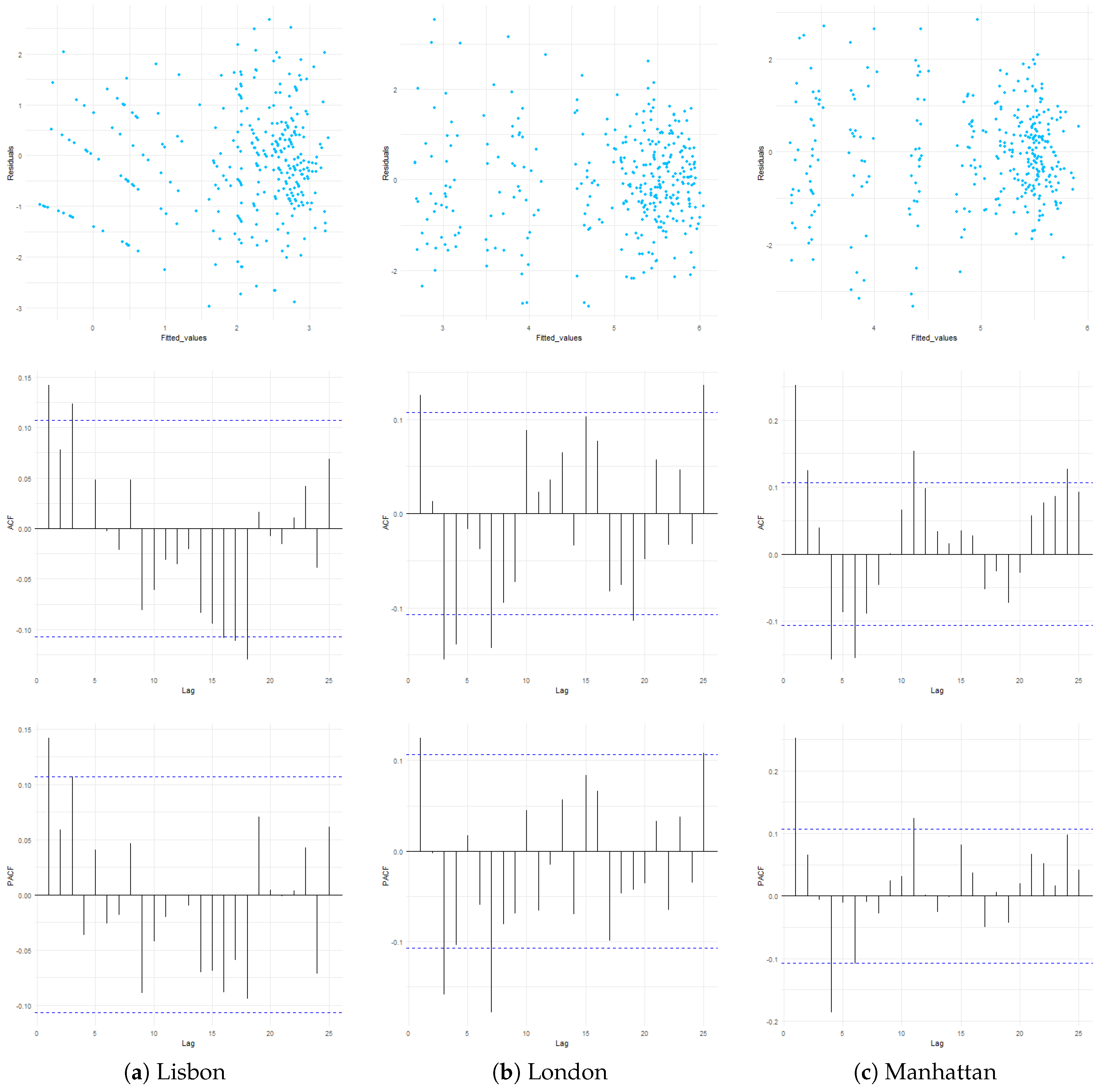
To evaluate the validity of the models and to identify departures from the statistical assumptions, we conducted a residual analysis. The results of the Shapiro-Wilk’s test are as follows: Lisbon: $W=0.996$, p-value = 0.65; London: $W=0.995$, p-value = 0.34; and Manhattan: $W=0.996$, p-value = 0.27; these results indicate that there is no statistical evidence to reject the null hypothesis that states the residuals of the models follow a Gaussian probability distribution. Additionally, Figure A1 shows the residuals versus the fitted values and autocorrelation function and partial autocorrelation function plots. We note that no apparent patterns arise from the relation between residuals and adjusted values and that the residual autocorrelation is not significant.

For each city, we built a multitype spatial point pattern, labelling each location with the hour when a user created the corresponding tweet. Figure 4 shows the distribution of the number of events for each mark, displaying the dynamics of the social media activity through the day. We established the length of the smaller side of the rectangles that circumscribe the city of Lisbon, London’s metropolitan area, and the island of Manhattan. Based on those lengths, we defined the maximum distances ($r_{{}_m}$) to estimate the L-Besag function. We worked with a sequence of values from 0 meters up to $r_{{}_m}$ with intervals of 25 meters.

Table 7. Distance parameters for estimating the second-order summary statistics for the hourly multitype spatial point patterns of tweets in the three studied cities

City	Length of the Shorter Side	$1/4$ of the Length	${\mathit{r}}_{{}_{\mathit{m}}}$	m
Lisbon	11,530.11	2882.53	2875	115
London	44,819.03	11,204.76	11,200	449
Manhattan	30,153.90	7533.96	7525	302

shows a summary of the obtained ranges. We then estimated the centered version $\widehat{L}(r)-r$ of the function, for every hourly formed spatial point pattern, over the set of those distances.

We obtained the functional representation of those estimations by using functional blocks of 117, 451, and 304 for Lisbon, London, and Manhattan, respectively, and a roughness penalty with a smoothing parameter of $\lambda =0.00001$. We then calculated the FPCA over the smoothed curves and kept the first two principal scores since together they contributed more than 70% of the variability in the three scenarios. Additionally, to disclose more significant components of variation, we rotated the functional principal components with the VARIMAX rotation algorithm [74]. Finally, we obtained a dendrogram by applying agglomerative hierarchical clustering through Ward’s method on the matrix of dissimilarities computed with the Euclidian distance between the scores.

Figure 8, Figure 9 and Figure 10 present the results of the spatio-temporal data analysis approach in the three studied urban scenarios. In the case of Lisbon, the smoothed functions reveal schemes of spatial clustering for almost all the considered distances and hours of the day, except for the case of the events registered at 04:00, whose curve decreases rapidly and reaches negative values after $1.75$ km. In addition, those functional representations belonging to hours from midnight to early in the morning (light deep-sky-blue curves) are more irregular than those associated with later hours. The first two principal components retain $86.06$% and $7.84$% of the variability. As a functional principal component symbolizes variation over the average curve, the interpretation depends on this capability. Thus, since the first component takes negative values for distances up to 500 meters, approximately the variation of the mean of the hourly second-order summary statistics, the relationship is strongest for distances longer than this value, and the second component captures primarily variations in the hourly summaries up to $1.5$ km. Panel (c) of Figure 8 reveals that the spatial distribution, of the shared events at 04:00, is quite dissimilar in comparison with the behavior of the distributions for the other hours of the day. There are approximately three groups of hours for human activities, thus: (1) between 00:00 and 01:00, (2) from 02:00 to 07:00, and (3) at the rest of the hours.

The smoothed centered L-Besag functions for London show less irregularity than those for Lisbon. The curves also exhibit a pattern of spatial clustering for all distances and hours of the day. The functional representation for the hourly second-order summary statistics reveals marked differences between the curves associated with tweets generated in dawn hours to the curves from tweets shared in other periods of the day. The first two principal components explain $97.5$% and $1.73$% of the variability of the summary statistics. The first harmonic portrays a continuous increase of the variation of the mean function with the distance, mainly from 3 km. The distribution of the hours through the scatterplot of the first two functional principal components reveals that there are approximately four groups, three of them for early hours in the morning and the other for the rest of the day.

Similar to the other two cities, the obtained results for Manhattan indicate that the spatial arrangement of the collected geolocated tweets exhibits schemas of spatial clustering for every hour and for all distances. In addition, the smoothed curves that belong to hours after midnight until 05:00 exhibit more irregularity than those at other hours of the day. The first two harmonics explain $70.13$% and $26.17$% of the variability of the smoothed L-Besag’s functions. The first component reveals that the variation in the mean function of the second-order summary statistics is increasing for all distances higher than $2.8$ km, whereas the second component portrays increments of the variations up to $4.2$ km. The hourly data can be divided into four groups: one for activities performed from 00:00 to 02:00, another for 03:00 to 05:00, and the other two for later hours.

Finally, we obtained the intensity function of each mark of the multitype spatial point pattern by using bidimensional-KDE. We employed the quartic kernel and selected the bandwidth by using Scott’s method [77]. We then standardized all the estimated values and normalized them to a scale of 0–1 by subtracting their minimum and then dividing by their range. Figure 11, Figure 12 and Figure 13 display the estimations. In Lisbon, there is a persistent accumulation of the human-generated data in the southern area lying along the Tagus River; this location contains the main attractions within the city. On the other hand, London’s metropolitan area concentrates social media activity in the surrounding boroughs of the city of London, which contain tourist locations, large companies, and commercial areas. The island of Manhattan aggregates most of the Twitter activity in the direction southwest of Central Park to the limits with the Upper Bay and the Hudson River, in which Times Square, SoHo, and the Financial District, among other attractions, are located.

6. Discussion

We first examined the temporal distribution of the number of geolocated tweets per hour by using regression models for count data under the scope of the GLMs. We evaluated and found that in the three studied cities, the models have a better goodness of fit when we used the negative binomial distribution for the random component. This result implies that the counts exhibit a high heterogeneity, which reflects the complexity of the analyzed systems and agrees with as stated by [9]. We additionally detected strong temporal trends related to the day of the week and the hour of the day that reinforce the idea that people who publish geolocated tweets tend to develop their activities approximately at the same times. França et al. [1,35,44] studied social media data from London and Manhattan and identified areas with high social media activity and differences in behavior between weekdays and weekends and in hours of the day. However, those temporal patterns change between cities. Our results in the case of Manhattan show that the estimated model did not establish a significant difference in the days of the week, which is contrary to the findings in previous research. These divergences can be due to those aforementioned studies used a more extended period of data collection than ours, which allowed the authors to have a broader image of the urban dynamics, not just a two-week period in a summer, and their conclusions are based on frequencies while we used a more sophisticated approach that included regression modelling and statistical hypothesis testing. The dissimilarity of the frequency of people’s use of social media in the other two cities through the weekdays might be an effect of the unusual counts registered in the time series of Lisbon that increased the volume of human-generated data from Tuesday to Thursday. After a thorough review, we attribute the outlier occurring on 9 August 2017, at 19:00 to the prematch tweets of the Portuguese local soccer league between Benfica and Braga. Our approach also involved the estimation of parameters associated with autoregressive trends. The findings highlight that those temporal effects are also significant to explain the number of tweets and can be meaningful as a measure to anticipate the pressures of increasing the amount of human activity.

We then investigated the spatio-temporal distribution of the geolocated tweets. We linked elements of statistical analysis of spatial point patterns, FDA, and hierarchical clustering. We discovered that locations, where people create and share social media data, exhibit a pattern of spatial clustering for every hour during the day and for all considered spatial scales. This result agrees with the fact the people tend to visit the same places at the same times [6,7,16]. Furthermore, we detected that those schemes of clustering change through the day, being more similar from 08:00 to midnight and highly unlikely between midnight and early hours in the morning. We also found that the measures of spatial correlation through the time tend to be more homogeneous in short distances, at 500 m, 3 km, and $2.8$ km for Lisbon, London, and Manhattan, respectively. These values differ significantly with travel distance of 1.5 km reported in human mobility studies [5,6,7]. The behavior of the smoothed second-order summary statistics showed more uniform curves in London and more erratic curves in Lisbon, which might be an effect of the number of gathered tweets in each city in the two-week period. The analysis also revealed that the places where people share content in Twitter are in the same areas at the same hours, which is a common feature in the social conduct of humans. The irregular shape of the curves for dawn hours retained most of the variability of the L-Besag’s functions; as a consequence, this covered other relevant spatial effects that occur in different periods of the day.

We found some limitations in our research. One of the main issues was regarding the analysis of content data that has provided meaningful insights into the field of Twitter Analytics. The inclusion of semantics components of geolocated tweets in our approach would give additional information about the cities. However, that was not our primary goal. We aimed to understand the spatio-temporal distribution of where humans interact with their social networks as a proxy for human activity and avoid constraints related to the semantic analysis. On the other hand, the identification and elimination of shared content by machines, bots, and other sources that are not people is a complex task that restricts the analysis. Also, the short study period and the season when was located can distort the found patterns. The representativeness of the harvested sample through the Twitter API is just around one per cent of the overall activity. Finally, estimated models can vary greatly depending on population number, social structure, ethnicity, culture, traditions, and consumer preferences. Many control variables can enter modelling.

Our work has characterized the behavior of human-generated Twitter data in cities as a proxy for human activity. We have found temporal and spatial regularities, namely, autoregressive and long-term temporal trends, as well as, spatial clustering in various scales that can be used as a first step for developing more complex and reliable models to explain the underlying nature of urban dynamics, such as mechanistic models [46]. This approach would face the problem to estimate parameters of spatio-temporal models in large datasets in which the Bayesian techniques have taken in a boom since they allow developing complex models without imposing simplified structures [78]. Notably, the integrated nested Laplace approximations (INLA) has shown to be a fast and accurate algorithm in comparison with the conventional Markov chain Monte Carlo methods [79,80,81] that can analyze social media data.

On the other hand, considering our results, we suggest that an approach based on epidemic data can more effectively accommodate the presence of outliers and might even be capable of predicting them. Epidemic data are conceived as realizations of spatio-temporal processes with autoregressive behavior which do not come from planned experiments. Its observations, number of events, are not independent, and phenomena are only partially observed [82]. There is a high similarity with the distribution of the number of geolocated tweets. Those methods also include autoregressive trends and spatio-temporal structures in the estimation of the parameters of the models that might describe human social conduct more accurately. Our analysis has shown the data coming from the hours commonly dedicated to rest might hide spatio-temporal patterns in the behavior of the people in the cities at other times of the day. Therefore, we also suggest that to avoid the randomness associated with activity during those hours, the analysis of the human activity in cities should be restricted to the hours of the day where humans are more active and developing their daily life.

7. Conclusions

This research reviewed relevant literature in the field of human urban activity, social media analytics and summarized several components in its study, as well as reflections on the statistical methods to find urban patterns. It has been highlighted the potential opportunities and impact of the analytical approaches suggested for the analysis of Twitter data and the study of the spatio-temporal distributions related to the understanding of the human urban activity. These have mainly reflected on how the proposed methods address some of the current gaps in the field of statistical modelling of human activity regarding monitoring, modelling, and predicting urban dynamics patterns on a large-scale level.

We have proposed an alternative to studying the spatio-temporal distribution of geolocated tweets using statistical methods for answering several questions. It first focused on developing a meaningful approach to analyze a considerable amount of human-generated data. In that direction, it was found that regression modelling, spatial point patterns, FDA, and hierarchical methods can process data coming from social networks and discover and describe regularities in the distribution of the human activities in the cites.

Additionally, this work aimed to characterize temporal and spatial structures in the data to capture the spatio-temporal behavior of humans. The evaluated techniques showed that temporal trends and spatial autocorrelation are relevant to improve the goodness of fit in regression methods and adequately describe the spatial distribution of the places where people interact with social media, respectively. The analytical proposal was tested in three different cities to characterize and compare behaviors across those urban environments which allowed to gain information involving human conduct in cities with different structures and dynamics.

We have found that our approach was able to identify almost the same behaviors in a more straightforward way than alternatives developed in previous research. On the other hand, our proposal is looking for providing easily implemented and reproducible methods that can be automatized and thus, analyze a significant amount of geolocated data with the advantage of using more advanced techniques. Moreover, we included and statistically tested the effect of considering structures of spatio-temporal autocorrelation that might allow for predicting, monitoring and, simulating the activities accurately in the cities. For example, the inclusion of autoregressive parameters permits anticipates abnormal situations due to the pressure that immediate changes produce in the short-term forecasts.