Article

Climate Change and Its Attribution in Three Gorges Reservoir Area, China

1
College of Horticulture and Forestry Sciences/Hubei Engineering Technology Research Center for Forestry Information, Huazhong Agricultural University, Wuhan 430070, China
2
School of Geography and Information Engineering, China University of Geosciences, Wuhan 430074, China
*
Author to whom correspondence should be addressed.
Sustainability 2019, 11(24), 7206; https://doi.org/10.3390/su11247206
Submission received: 22 October 2019 / Revised: 10 December 2019 / Accepted: 12 December 2019 / Published: 16 December 2019

Abstract

:
Climate change in dam areas is one of the environmental problems associated with dams. However, the main factors and mechanisms that impact climate change in dam areas remain unclear. In this study, linear regression, the observed minus reanalyzed (OMR) method, and multi-source data are used to assess climate change in the Three Gorges Reservoir Area of China and investigate the main impact factors among the controversial factors (land cover change, environmental climate, and reservoir impoundment). Our results indicate that turning points of trend changes for annual fog days (FD), annual average temperature (T), and annual average relative humidity (RH) occurred at around 1996 during the period 1973–2013, and annual precipitation (PRE) suggested no obvious turning point. The change trends after 1996 were steeper than before 1996. These changes are mainly closely correlated with environmental climate. In particular, temperature was significantly correlated with environmental temperature (1979–2013: r = 0.799, p < 0.01), and their relationship was stronger after 1990 (r = 0.842, p < 0.01). Moreover, the turning point for FD, T, and RH also correlated with land use/cover change. In addition, reservoir impoundment showed an obvious humidification effect (OMR RH correlated with water area: r = 0.566, p < 0.01). Our findings support the view that climate change in dam areas is mainly affected by environmental climate changes.

1. Introduction

As human civilization has rapidly developed, the demand for water has become increasingly prominent, including water supplies, irrigation, flood control, navigation, and hydropower. A dam is an important project in the effective development and management of water resources. Consequently, dams have been widely constructed worldwide. By the end of 2006, there were 52,000 dams with heights of 15 m worldwide (including dams with heights between 15 and 30 m in China), which increased by approximately 38.32% compared with the number of such dams in 1986 [1]. We have witnessed a global boom of dam construction in the last 20 years [2]. Although the benefits of dams have been highlighted, environmental problems associated with dams have also attracted much attention. Examples include the landslide that occurred at Assar [3], extreme heat and drought that occurred at the Three Gorges Reservoir Area (TGRA) in China [4], extreme precipitation at the Owyhee Dam [5], and thunderstorms in Southeast Texas [6]. Both landslides and extreme weather have a direct or indirect relationship with regional climate change. The obvious impacts of climate change underlie concerns regarding how the climate changes and what influences those changes in dam areas.
Many studies have been done to investigate climate change in dam regions, e.g., temperature and humidity studies at Ermenek Dam in Turkey [7]; changes of temperature, precipitation, evaporation, and wind speed in Gökpınar Dam in Turkey [8]; evaporation and precipitation changes in the TGRA [9]; and surface moisture and precipitation change at Owyhee Dam in the US [10]. These studies indicate that climates in dam areas have indeed changed, but what caused these changes is still not very well understood.
Generally, regional climate is determined by local variables and environmental climate and their interactions, including the natural microclimate, human activities, and atmospheric circulation. Environmental climate in this paper is defined as the climate of the climate zone in which an area is located (environmental temperature or humidity or precipitation all present the temperature, humidity, or precipitation of the climate zone in which the area is located.) Moreover, the climate is affected by the surrounding upper-air atmosphere and global atmospheric circulation. Therefore, climate at the dam areas should also depend on geographical location, human activities (dam projects and other projects), and environmental climate. To further investigate, it was found that large dams influence local climate, such as air humidity, and wind speed at Sobradinho Dam in Brazil [11] and precipitation in the 92-dam area in the Koppen-Geiger regions in the US [12]. In addition, land use/cover change (LUCC) caused by dam projects was suggested to affect local climate in Yamula Dam in Turkey [13] and in the TGRA [14]. It is believed that increased areas of open water will increase the evaporation at a certain region [15,16]. In dam areas, increased areas of water caused by reservoir impoundment then altered local precipitation [17,18]. The combination of dam reservoir size and LUCC patterns was also found to affect precipitation [19]. However, there are differences at different dam areas with respect to the attribution of local climate change. What is interesting is that, even in the same dam area, there is debate about the attribution of climate change. As in a case regarding the TGRA, changes of precipitation were suggested to be affected by LUCC [14], atmospheric circulation [20], and reservoir impoundment [17] in three separate studies. These studies indicate that factors that affect climate change in dam areas are various and complex, which makes it difficult to identify the attribution of the changes.
The Three Gorges Reservoir, known globally for its Three Gorges Dam Project (TGDP), is a typical artificial reservoir. With the implementation of the TGDP, many programs, such as the Resettlement Program [21], the Grain-to-Green Program, and the Natural Forest Conservation Programme, were initiated at the TGRA [22,23]. As a result, land cover of this area has undergone rapid changes in recent years, including water area increase caused by impoundment. Therefore, in this paper, the TGRA is taken as a case study to investigate climate change and its attribution to the dam regions. In addition, it has been documented that there were spatial gradients of climate effects of the artificial reservoir in horizontal and vertical directions [12,24]. The low elevation area of the TGRA is mainly concentrated near the reservoir, and the area of the TGRA below 500 m above sea level was thus chosen as the study area in this paper. We collected observed data for average monthly temperature, average monthly air relative humidity, monthly precipitation, and monthly fog days in the study area and estimated the impact of the controversial contributing factors on climate change using observation and reanalysis data and land cover maps of the TGRA. Moreover, one method—the observed minus reanalyzed (OMR) method proposed by Kalnay and Cai [25]—has been documented to be an effective means for investigating the effects of land use/land cover changes on climate change [26,27]. Therefore, in this study, the OMR method was used to investigate the effects of land use/land cover changes on climate change. We aimed to answer the following three questions: 1) How did the climate change before and after the TGDP? 2) How did the climate changes relate to reservoir impoundment and the LUCC caused by the TGDP? 3) Which of the controversial factors are the main contributing factors for the climate changes in the TGRA?

2. Materials and Methods

2.1. Study Area

The TGRA is located in the upper reaches of the Yangtze River (Figure 1) between latitudes 28°56′ N-31°44′ N and longitudes 106°16′ E-111°28′ E and has a total area of 58,000 km2 [28,29]. The area below 500 m above sea level in the TGRA is the study area, with a total area of 20,548.51 km2. The construction period of the TGDP was from 1993 to 2009. The reservoir was impounded three times, in 2003, 2006, and 2009. The total reservoir surface water area reached 1080 km2 and total storage reached 39.3 billion m3 at a water level of 175 m. Approximately 1.3 million people were relocated from the inundated area onto higher ground [30]. The climate is subtropical, with an average annual temperature of approximately 17.8°C and an average annual rainfall of approximately 1100 mm. The region displays complex topography, with a diverse range of vegetation and categories of land use, and is an important ecological zone in China.

2.2. Data

For the surface observed climate data, we selected the monthly mean temperature, monthly mean precipitation, monthly mean air relative humidity and monthly fog days during 1973–2013 for 41 available stations over the TGRA and contiguous provinces. These data were downloaded from the China Meteorological Data Sharing Service Web (http://data.cma.cn/). Of these 41 stations, only 14 stations were located in the study area (Figure 1).
For the environmental climate data, because the reanalysis surface data are strongly influenced by the surrounding upper-air atmosphere and are insensitive to land cover changes [31,32], the reanalysis data were treated as a product of atmospheric circulation in this study. Therefore, the surface reanalysis data in this study were used as the environmental climate data and were downloaded from the NCEP-NCAR Reanalysis (NNR) data web site (https://www.esrl.noaa.gov/psd/data/reanalysis/). We collected the homochromous global surface monthly mean temperature, monthly mean precipitable water and monthly mean air relative humidity gridded at the 0.995 sigma level and on 2.5° Gaussian boxes. Because there were no data for fog days from NCEP-NCAR, we did not use the reanalysis data of fog days.
The LUCC data were derived from Landsat TM/ETM+/OLI images (2013 v2 at 30 m resolution) using the supervised classification and artificial visual correction method [33]. There were five maps in 1990, 1995, 2000, 2005, and 2010, and each map was recognized to have nine land categories—farmland, coniferous forest, evergreen broad-leaved forest, deciduous broad-leaved forest, mixed broadleaf conifer forest, shrub land, grassland, residential land, and water. The other lands to be built and unused were identified as bare land. Shrub land is evergreen or deciduous broad-leaved shrubs, and most are bamboos, teas, and citrus. The grassland is mainly alpine meadow, and the grassland area in the low altitude area of the TGRA is small [34]. Our study area was extracted from ASTER Digital Elevation Model (DEM) (30 m resolution) data from the US Geological Survey website (http://www.usgs.gov).

2.3. Method

2.3.1. Data Processing

(1) Meteorological data processing
We linearly interpolated the gridded NNR data to each observational site and then obtained monthly NNR data for the corresponding sites. All annual data were calculated using monthly data for both the observations and interpolated reanalysis, and each meteorological factor anomaly and accumulative anomalies were separately calculated. Annual fog days, annual average temperature, annual average relative humidity, annual precipitation, and annual precipitable water were defined as FD, T, RH, PRE, and PRW, respectively. The annual meteorological factors for NNR were separately defined as Tnnr, RHnnr, and PRWnnr.
(2) Land use/cover data processing
Extracting the LUCC map of the study area was based on DEMs using ArcGIS spatial analysis tools. LUCC data were classified into the following five categories: urban-built land (Urb), forestry land (Frt), agricultural land (Agr), water land (Wtr), and bare land (Bal). The residential land was classified as Urb, the bare land and water were still classified as Bal and Wtr, the grassland and farmland were classified as Agr, and the others were classified as Frt. The area of each type was calculated based on pixel size and numbers of pixel to obtain the LUCC values in 1990, 1995, 2000, 2005, and 2010. The yearly LUCC data for the 21-year duration (1990–2010) were linearly interpolated from the five-year LUCC data for the period.

2.3.2. Climate Trend Slope

Anomalies were used to reduce the influence of altitude on the results. Annual climate change trends were calculated based on the time series of observed anomalies for the total study area [26].
The slope of the linear regression model was applied to describe the changing trend for each meteorological variable,
x = b + a t   ( t = 1 ,   2 ,   ,   n ) ,
where x is a meteorological variable with n samples, t is the time, a is the modelled slope (per year), 10*a is the climate trend slope, and b is the intercept of the regression model.
A negative slope generally implies a decreasing trend, whereas a positive value suggests an increasing trend. We used F and t statistics to test the significance of the model and slope in the regression analysis, respectively (tested at the significance level to 0.05).

2.3.3. Abrupt Climate Detection

We used cumulative anomalies curves and Mann–Kendall (MK) tests [35,36] to obtain the climate jump points and tested at the significance level to 0.05.
(1) Cumulative anomaly curve
The cumulative meteorological variable anomaly should have the advantage of effectively filtering some of the high-frequency noise without actually losing any of the signal [37]. Thus, the cumulative anomaly curve indicates the trend, and when the trend turns significantly, the turn point represents the abrupt point,
x = t x t 1   ( t = 1 ,   2 ,   ,   n ) ,
where x is a meteorological variable with n samples and t the time.
(2) MK detection
The MK test is a method used to detect abrupt climate change with a wide detection range and a high degree of quantification as the highlight [35,36,38].
For time series X of meteorological variables with n samples, a rank sequence is constructed using the following equation:
s k i = 1 k r i   ,               r i { 1 ,   x i > x j 0 ,   e l s e   j = 1 ,   2 ,   ,   i ,
where Sk is the cumulative sequence of the number of values at the ith time greater than that at the jth time. Under the assumption of random independence of time series, UFk is defined as follows:
U F k = s k E ( s k ) V a r ( S k )   ,                 k = 1 ,   2 ,   ,   n ,
where UF1=0, and E(Sk) and Var(Sk) are the mean value and variance of Sk, respectively. E(Sk) and Var(Sk) are calculated as follows:
E ( s k ) n ( n + 1 ) 4   ,                                 V a r ( S k ) n ( n 1 ) ( 2 n + 5 ) 72
UF is calculated in time-series order (x1, x2, …, xn). According to the reverse order of time series (xn, xn-1, …, x1), UB is calculated using the same method of calculating UF, and UB1=0.
Setting the significance level to 0.05, the value of the critical line is then U0.05=±1.96. UF, UB, and the two critical lines are drawn on the same graph. If UF>0, it indicates that the sequence shows an upward trend, and if it is less than 0, it shows a downward trend. If there is an intersection between UF and UB, and the intersection is between the critical lines, the time corresponding to the intersection is the time when the abrupt change starts.

2.3.4. OMR Method and Correlation Analysis

Because of the effect of the surrounding upper-air atmosphere and global atmospheric circulation and insensitivity to land use change [25], NNR data were treated as the product of atmospheric circulation in this study, and the OMR method was used to investigate the effects of land use/land cover changes on climate change. PRW was referred to as the total amount of water vapor contained in the unit atmospheric column [39]. Therefore, the value of precipitation minus precipitable water was still precipitable water, and the observed PRE minus reanalyzed PRW was thus OMR precipitable water (OMR APRW). We calculated the anomalies of the OMR T (OMR AT), OMR RH (OMR ARH), and OMR PRE (OMR APRE) and their trends using the observed and reanalyzed meteorological factors. We comparatively analyzed the change trends of the observed, reanalysed and OMR meteorological factors. We related the observation trends to the NNR trends in different periods to investigate the relationship between climate change in the TGRA and environmental climate change.
According to the time series of observed anomalies and LUCC type area percentages, we related the observation trends to the LUCC trends [40] to investigate the relationship between climate change in the TGRA and LUCC. We analyzed the correlation between the observed meteorological factors and the LUCC. Then, we correlated the OMR meteorological factors with the LUCC to further investigate the relationships between climate change and LUCC in the TGRA. All correlation analyses were conducted at the 95% confidence level.

3. Results

3.1. Dissection of Annual Observed Meteorological Factors Variability

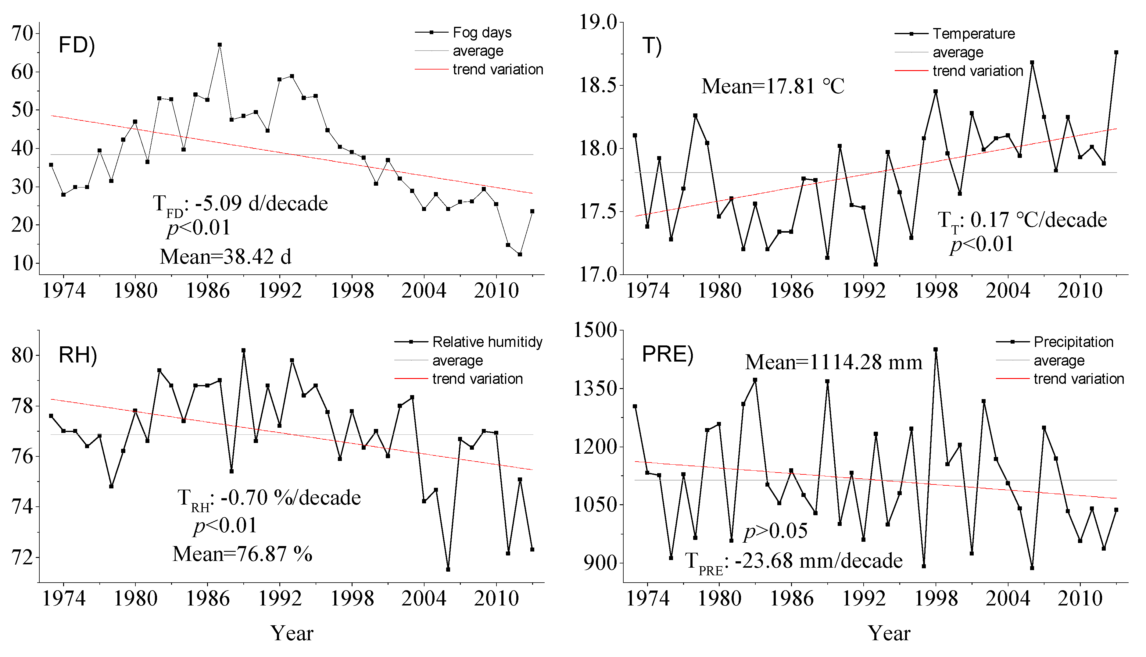
According to the statistical analysis of meteorological data from 1973–2013, the average number of FD was 38.42 d, the average RH 76.87%, the average T 17.81°C and the average PRE 1114.28 mm. During the past 41 years, FD significantly decreased (−5.09 d/decade, p < 0.01), and there was an obvious peak of the time curve between 1985 and 1994 (Figure 2(FD)). T significantly increased (0.17°C/decade, p < 0.01), and the minimum value appeared around 1992 (Figure 2T). At the same time, RH significantly declined (−0.7%/decade, p < 0.01), and the curve showed no obvious peaks and troughs; however, there was a significant decline in 1993, and the minimum value appeared in 2006 (Figure 2(RH)). PRE showed an irregularly fluctuating declining trend (–23.68 mm/decade), and the downward trend was not significant (Figure 2(PRE)). These results indicated that the time series of FD, T, and RH turned in the early 1990s, whereas PRE had no obvious turning points.
As the construction of the dam under study took place between 1993 and 2009, the trend changes in climate were statistical analyzed from 1973 to 1992 (pre-dam), from 1993 to 2009 (dam period), and from 2010 to 2013 (post-dam), and the results are shown in Figure 3. In the pre-dam period, FD was significantly increasing at a rate of 13.33 d/decade, and the mean of FD was 44.31 d; T was slightly decreasing at a rate of 0.14 °C/decade, and its mean was 17.61 °C; RH was slightly increasing at a rate of 0.86 %/decade, and its mean was 77.53 %; and PRE was slightly decreasing at a rate of 29.15 mm/decade, and its mean was 1128 mm. In the dam period, FD was significantly decreasing at a rate of 19.74 d/decade, and its mean was 36.07 d; T was significantly increasing at a rate of 0.44 °C/decade, and its mean was 17.97 °C; RH was significantly decreasing at a rate of 2.24 %/decade, and its mean was 76.73; and PRE was slightly decreasing at a rate of 36.59 mm/decade, and its mean was 1126.57 mm. In the post-dam period, FD was slightly decreasing at a rate of 8.1 d/decade, and its mean was 18.95 d; T was not significantly increasing, with a rate of 2.36 °C/decade, and its mean was 18.15 °C; RH was not significantly decreasing, with a rate of 10.93 %/decade, and its mean was 74.11 %; and PRE was not significantly increasing, with a rate of 138.46 mm/decade, and its mean was 992.76 mm.
Comparing climate change trends over different times, the results showed that trends of the four meteorological factors in the dam period were steeper than that in the pre-dam period (Figure 3). FD (k = 13.33 d/decade turned to k = −19.74 d/decade) and RH (k = 0.86 %/decade turned to k = −2.24 %/decade) changed from rising to falling. On the contrary, T (k = −0.14 °C/decade turned to k = 0.44 °C/decade) changes from falling to rising. PRE (k = −29.15 mm/decade turned to k = −36.59 mm/decade) fell faster. Trends of T (k = 2.36 °C/decade) and RH (k = –10.93 %/decade) in the post-dam period were same as those in the dam period, but were steeper; the trend of FD (k = −8.1 d/decade) in the post-dam period was also that same as that in the dam period, but with a gentle change; and the trend of PRE (k = 138.46 mm/decade) in the post-dam period was contrary to that in the dam period, and was steeper.
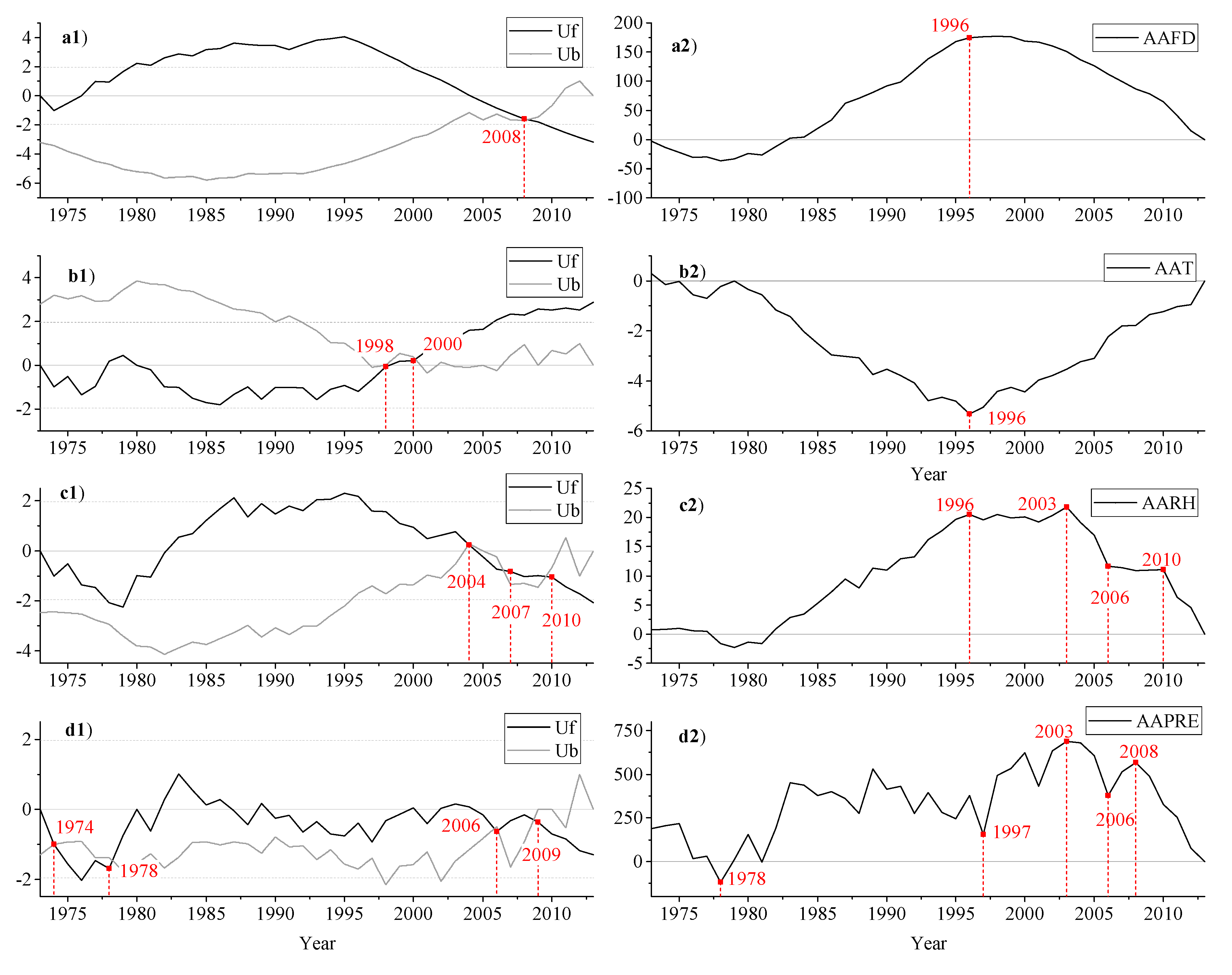
Figure 4 shows the curve changes of the MK test and the accumulative anomalies of FD, T, RH, and PRE. The result of the MK test indicated that a turning point of FD appeared in 2008 (Figure 4(a1)), but the curve of the accumulative anomalies of FD (AAFD) showed that the point appeared at around 1996 (Figure 4(a2)). The MK test of T indicated that turning points occurred in 1998 and 2000 (Figure 4(b1)), but the accumulative anomalies of the T (AAT) curve showed that the point occurred at around 1996 (Figure 4(b2)). For RH, the MK test showed that three turning points occurred in 2004, 2007, and 2010 (Figure 4(c1)); however, the accumulative anomalies of the RH (AARH) curve showed that the turning points occurred in 1996, 2003, 2006, and 2010 (Figure 4(c2)). For PRE, the MK test showed that there were two turning points, in 2006 and 2009 (Figure 4(d1)), but the accumulative anomalies of the PRE (AAPRE) curve showed that there were no obvious turning points (Figure 4(d2)). This was because the differences in the results of the MK test and the accumulative anomalies of FD, T, RH, and PRE indicated that some of the turning points were false.
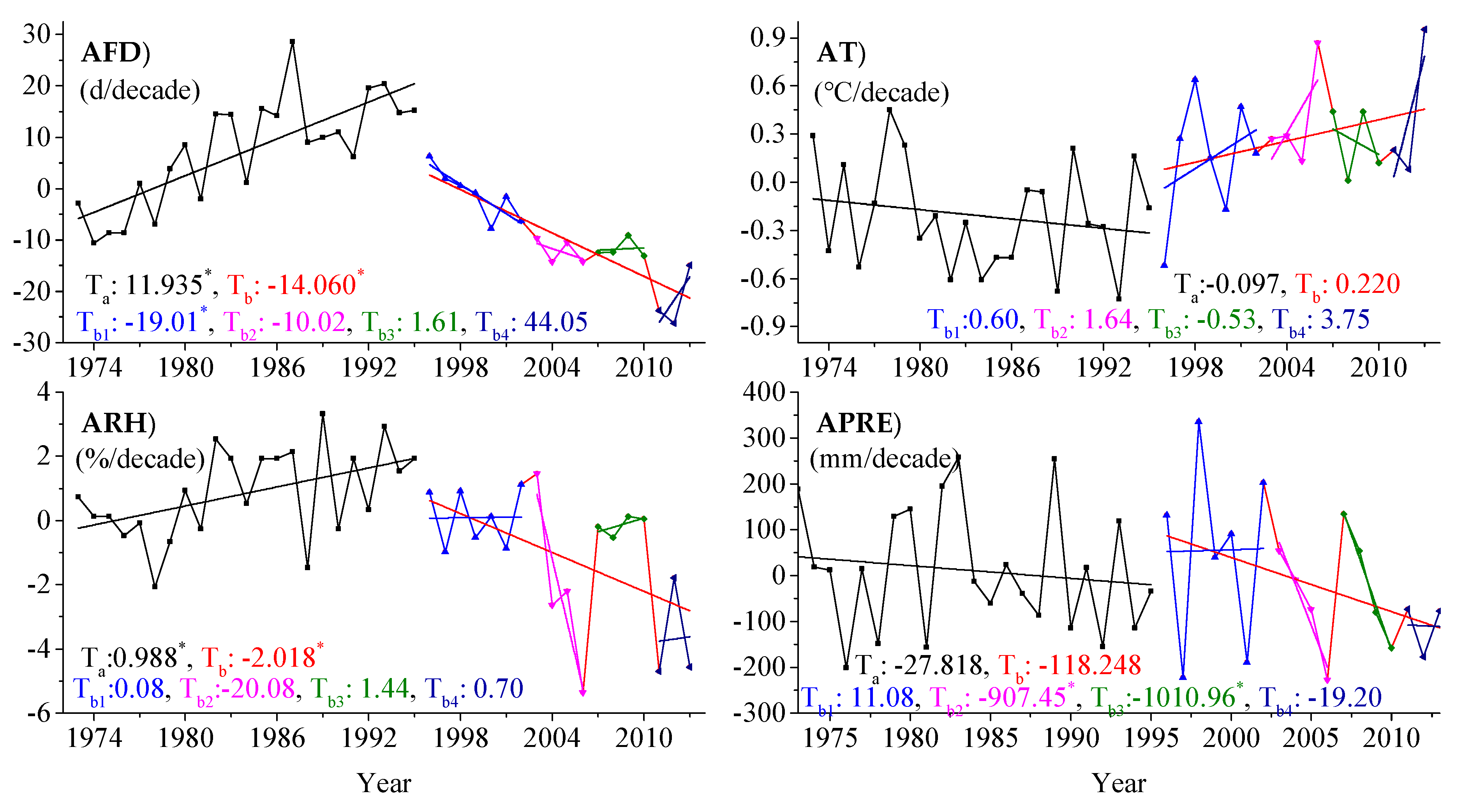
To further investigate the turning points, the trends of anomalies for FD (AFD), T (AT), RH (ARH), and PRE (APRE) were analyzed based on the following years: 1996, 2003, 2006, and 2010. The change trends of the four meteorological factors after 1996 were steeper than before 1996 (Figure 5), which suggested that 1996 was indeed a turning point. The anomalous trends of FD, T, RH, and PRE were compared during several periods from 1996 to 2013. Although most change trends were not significant, FD showed a gradual trend of decline after 2003 and a sharp trend of decline from 1996 to 2002. Changes of AT were different in different periods, but all these trends were not significant. Additionally, all changes of RH were not significant over the four periods, and the change trends of APRE were only significant in the periods 2003–2006 and 2007–2010. The results show that the years 2003, 2006, and 2010 were not turning points for FD, T, RH, and PRE; however, all of these trends changed during these periods.

3.2. Climate Changes Associated with Environmental Climate Changes

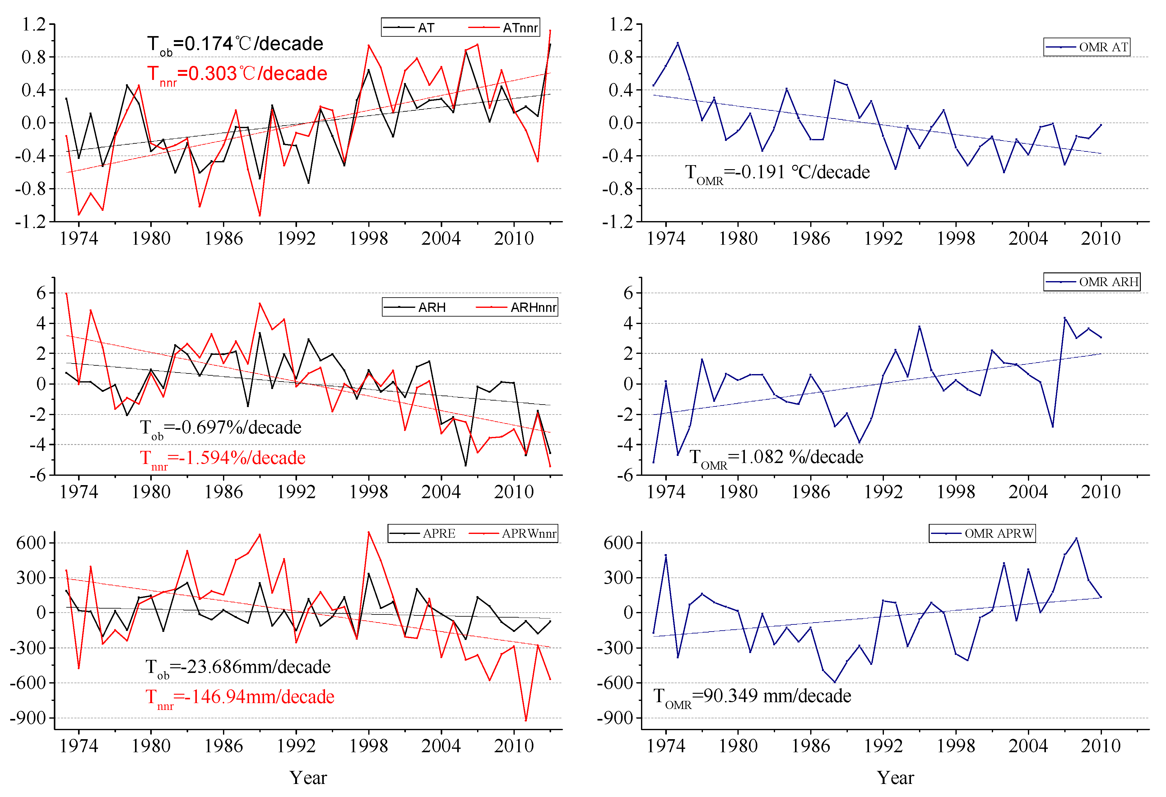
From 1973 to 2013, the trends of observations were consistent with those of the NNR (Figure 6) and indicated that changes of T, RH, and PRE were affected by the environment climate. Correlations between the observations and the NNR were also compared in different periods (Table 1). For long-term (1973–2013) research, FD was positively correlated with RHnnr (r = 0.557) and PRWnnr (r = 0.62), T was positively correlated with Tnnr (r = 0.799) and negatively correlated with RHnnr (r = −0.513) and PRWnnr (r = −0.318), RH was positively correlated with RHnnr (r = 0.635) and PRWnnr (r = 0.641) and negatively correlated with Tnnr (r = −0.371), and PRE was positively correlated with PRWnnr (r = 0.476) and RHnnr (r) = 0.333). For short-term research, the year 1990 was treated as the segment point of the time series to be consistent with the period of the land cover data. Before 1990, FD was positively correlated with PRWnnr, T positively correlated with Tnnr, RH positively correlated with RHnnr and PRWnnr, and PRE not significantly correlated with the NNR. After 1990, FD was negatively correlated with Tnnr and positively correlated with RHnnr, T positively correlated with Tnnr, RH positively correlated with RHnnr and PRWnnr and negatively correlated with Tnnr, and PRE not significantly correlated with the NNR. The results showed that the changes of FD, T, and RH were affected by the environment climate for both long and short-term periods, but PRE showed a correlation with the environment climate only for the long term. Besides, RH was related to FD, T, RH, and PRE (Table 1). In addition to being correlated with RH, FD and T were correlated with each other in the periods 1990–2010 and 1973–2013, whereas PRE was only correlated with RH. These results indicated that changes of FD, T, RH, and PRE were also correlated with local meteorological factors. However, there were differences in the correlation significance levels and the correlation coefficients between the NNR factors and the observations (FD, T, RH, and PRE).
Considering the correlation significance level and the correlation coefficient (Table 1 and Table 2), the correlation of FD with RH was the strongest for both long and short-term periods. However, FD before 1990 was mainly correlated with RH, and the correlation with RH, T, and RHnnr after 1990 was stronger than with the other factors. The results showed that change of FD was mainly affected by RH, but this effect had decreased after 1990. T was mostly related to Tnnr on all temporal scales in this study, followed by RH. However, the relationship with RH before 1990 was much weaker than the relationship with RH after 1990. These showed that change of T was mainly affected by environmental climate and that this effect had been strengthened after 1990. Across each temporal scale, RH was closely correlated with FD. Moreover, FD was closely related to T after 1990 and during the entire 41-year period (1973–2013), and it was closely related to the PRE before 1990. These results indicated that changes in RH were mainly affected by local T and PRE, which were mainly affected by PRE before 1990 and mainly affected by T after 1990. PRE was most closely related to RH at all temporal scales. PRE was only significantly related to RH for the short term (1973–1989 and 1990–2010), but it was also closely related to the precipitable water of the environment climate for the long term. These results indicated that the PRE was mainly affected by local air humidity; however, the relationship after 1990 was weaker than it was before 1990.

3.3. Climate Changes Associated with Land Use/Cover Change

From 1973 to 2013, the trend of observation change was gentler than that of the NNR data (Figure 6). The annual average temperatures of observations rose more slowly, and the annual average relative humidity and annual precipitation dropped more slowly. When the NNR values were subtracted from the observed values, the annual average temperature showed a decreasing trend, and the annual average air relative humidity and annual precipitation showed an increasing trend (Figure 6). These trends indicated that LUCC altered the regional climate changes.
From 1990 to 2010, the largest land cover types were always agricultural land (Agr) and forestry land (Frt), and these two main land categories changed significantly (Figure 7a). The water (Wtr) area showed a significant increasing trend, and the trend after 2005 was steeper than before 2005 (Figure 7b); the area of urban-built land (Urb) was linearly increasing, and there was no obvious turning point. As the turning points appeared in 1995 for Frt and Agr, the A/F also showed a turning point in 1995 (Figure 7b). These results indicated that the area of vegetation (area of forest and agriculture land) decreased from 94.22% in 1990 to 84.95% in 2010 and was converted into Urb and Wtr in the study area. Compared with 1990, Agr decreased by 32.85% in 2010. In contrast, Frt increased by 123%, Ubrl increased by 439%, and Wtr increased by 90% for the same period. The results of LUCC meant that changes of each land use category significantly exceeded 10% from 1990 to 2010 in the study area. In this case, the relationship between LUCC and regional climate change was analyzed (Table 3). FD was negatively correlated with Urb (r = −0.89, p < 0.01), Frt (r = −0.907, p < 0.01), and Wtr (r = −0.746, p < 0.01), and positively correlated with Agr (r = 0.892, p < 0.01) and A/F (r = 0.94, p < 0.01). T was negatively correlated with Agr (r = −0.512, p < 0.05) and A/F (r = −0.563, p < 0.01), and positively correlated with Urb (r = 0.511, p < 0.05) and Frt (r = 0.526, p < 0.05). RH was negatively correlated with Urb (r = −0.491, p < 0.05) and Frt (r = −0.514, p < 0.05), and positively correlated with Agr (r = 0.49, p < 0.05) and A/F (r=0.533, p < 0.05). These results revealed that the relationship between FD and LUCC was closer than that between T and LUCC and between RH and LUCC. It was documented that LUCC had a greater effect on FD than T and RH. For T, the relationship between T and A/F was greater than that of T and the other land cover types. The results revealed that T was more sensitive to changes of A/F than those of other land use types. There was no significant relationship between precipitation and LUCC, which revealed that LUCC had affected the changes of FD, T and RH but had no significant effect on PRE.
Since there were no FD data for NNR and since PRE was not significantly correlated with LUCC, only the OMR T and OMR RH were further correlated with LUCC (Table 4). OMR T was not significantly correlated with LUCC, and OMR RH was positively correlated with Urb (r = 0.464, p < 0.05) and Wtr (r = 0.566, p < 0.01), and negatively correlated with Agr (r = −0.441, p < 0.05). These results revealed that LUCC had no significant effect on T, but Urb, Agr and Wtr had significant effects on RH. The relationship between RH and water area was greater than its relationship with Urb and Agr, which revealed that the impact of water area change on RH was greater than that of Urb and Agr on RH in this study area from 1990 to 2010. These results also revealed that the conversion between vegetation types had no significant effect on T and RH.

4. Discussion

4.1. Climate Change of the Three Gorges Reservoir Area

Climate in the TGRA in different periods showed different changes (Figure 3). Trends of T and RH in the dam and post-dam periods were contrary to the trends in the pre-dam period, and at faster rates. For FD, the trend in the dam period was also contrary to that in the pre-dam period, and at a faster rate. However, the trend rate turned to gentler than it was in the dam period. Meanwhile, although the trend of PRE in dam period was the same as in the pre-dam period, but at a faster rate, the trend began to climb in the post-dam period. This may mean that the programs in the dam period altered the local climate, and the decreasing trend of FD turned gentle, which was caused by increased PRE in the post-dam period.
However, because we have no more weather station data, it is difficult to confirm whether the climbing trend of FD in the post-dam period was caused by increased PRE. In addition, our further results indicated that 1996 was a turning point for the change trends of the three factors (FD, T, and RH), which is consistent with previous studies [41,42,43]. However, there was no obvious turning point for PRE. Two possible reasons may explain this result of PRE. First, as the Three Gorges Reservoir area has a humid mid-subtropical monsoon climate [33,34], the precipitation was affected by warm humid air masses from the Pacific Ocean and cold and dry air masses from Asia and Europe. Hence, change of annual precipitation is determined by the interaction of the two masses. If the interaction of air masses is constant, the annual precipitation will not change significantly. Second, precipitation may change in seasons or monthly, however, the precipitation in this study was total amount of year, which means change of annual precipitation may cover the change of seasonal or monthly precipitation. Therefore, PRE had no obvious turning points.
In addition, we made two new discoveries—(1) the MK test result is inconsistent with that of the accumulative anomalies test, and (2) there are several points that need attention, including 2003, 2006, and 2010 (Figure 4). The change trends of FD, T, and RH had markedly abrupt turns, which are similar to the temperature changes in high latitudes plotted by Goossens and Berger [44]. Moreover, some studies suggest that when the MK method was adopted to test abrupt turns, the detected turning points are uncertain and may be erroneous turning points [38,45]. The MK test in this paper may have produced false turning points for the detection of abrupt climatic change that were different from the results of the accumulative anomalies test (Figure 4). However, the MK method can better reduce the errors caused by human factors and result in a higher degree of quantification, and researchers are thus inclined to use MK test for abrupt climate change detection tests, always in cooperation with other detection methods to prevent the generation of errors [38]. This justified the adoption of both the MK test and the accumulative anomalies method for climate change detection in this study (Figure 4). Although there were differences in the results of the two detection methods, when combined with the results of abrupt change detection (Figure 4) and the original observation changes (Figure 2 and Figure 3), it was still ascertained that the turning points of the change trends of FD, T, and RH appeared around 1996.
Besides, the MK and accumulative anomalies test results indicated that 2003, 2006 and 2010 were turning points for RH (Figure 4(c1,c2)), although the segmentation trend changes among these points were not significant (Figure 5(ARH)). These results may be affected by the following two factors. One is extreme weather, such as the strong precipitation in the Yangtze River valley in the summer of 1998 and the extreme drought and heat in the southwest of the TGRA in the summer of 2006 [4]. The second was the three impoundments of the TGRA (in 2003, 2006, and 2009). Figure 2 and Figure 5 show that the TGRA experienced a hot and wet year in 1998 and a hot and dry year in 2006. Therefore, RH in the study area was relatively high in 1998 and relatively low in 2006. These extreme weather conditions led to an abnormal year in the TGRA, and the segmentation trend changes of RH were not significant. The impoundments of the reservoir expanded the area of water from 4.41% (1990) to 8.38% (2010). In general, under the same conditions, increased areas of open water will increase the evaporation at a certain region and then cause an increase in air humidity [15,16]. Therefore, the impoundment of the Three Gorges Reservoir had a certain influence on RH in the TGRA. The influences of these two aspects also suggested that the climate changes in the TGRA were affected by both the environmental climate and surface cover changes.

4.2. Comparison of the Impact Factors on Climate Changes

Our results indicated that T, RH, and FD were affected by environmental climate and local LUCC in the study area. However, our results also revealed that the correlation between meteorological factors and changes in some land cover categories were contrary to results from previous research. For example, the relationship between T and forestry land (Frt) should be negative because of the carbon sequestration of vegetation [46]—the larger the forestry land area and the more carbon sequestration, the stronger the cooling effect [47]. Another example is that RH and Frt should be positive because of the transpiration of vegetation [48]—the larger the forestry land area and the greater the evaporation of transpiration, the greater the air humidity. The third example is that RH and urban-built land (Urb) should be negative as well because of the dry-island effect of urban areas [49]—the larger the urban area and the greater the dry-island, the stronger the dry effect. However, the opposite results appear in Table 3 and Table 4.
This inconsistency will be explained below. Taking the relationship between T and Frt as an example, the increasing forest area should cool down temperatures, but in this study, it was found that the temperatures increased as Frt increased (Table 3). This can be explained by the three following aspects: (1) The relationship between T and Frt was only the correlation analysis of the change trend, and changes of T and Frt all showed an upward trend and thus were positively correlated. (2) As the Grain-to-Green Programme and the Natural Forest Conservation Programme were initiated in the TGRA [22,23], the main trees of the Grain-to-Green Programme were coniferous species, and these coniferous species for afforestation may have increased atmospheric temperature [50]. Therefore, species conversion of forest land in this study may have had a positive influence on temperature. (3) In this study, although the forest area increased, the vegetation area (involving forest and agriculture land) in the entire study area was reduced because of the increasing area of water and towns; consequently, the cooling effect of vegetation on the temperature in the entire study area was even weaker than before. Besides, T was affected by both environmental climate and local LUCC, which indicates that the correlation between T and LUCC cannot be regarded as a causal relationship. T was significantly correlated with LUCC, but this only indicated that temperature in the study area may be related to LUCC. Therefore, we did not focus on positive or negative change directions but only considered the strength of the relationships. The focus of the relationships between LUCC and other meteorological factors was the same as that between LUCC and T.

4.2.1. Temperature Change Analysis

LUCC changes over 10% can significantly impact regional climate [51] and the observation minus reanalysis (OMR) method can effectively reflect the impact of land surface cover on climate changes [26,27,52]. The areas of each land cover category exceeded 10% in this study (Figure 7). Consequently, LUCC influenced the climate in the study area.
For temperature, the results of declining OMR AT (Figure 6) and the correlation with LUCC (Table 3 and Table 4) revealed that changes of land cover mitigated the warming effect, but the effect was not significant, which is consistent with previous studies [17,53]. Our results also indicated that changes of the area ratio of agricultural and forestry land had an indistinct influence on temperature (Table 3 and Table 4). Furthermore, study results of Silvério et al. [47] indicated that forest-to-crop transitions increased land surface temperature. In the study area, some agricultural land has transformed into forestry land. These results revealed that optimization of vegetation structure contributed to climate change mitigation. In addition, since both temperature and OMR temperature had no significant relationship with the change of water area in the study area (Table 3 and Table 4), impoundment of the reservoir had no significant influence on temperature change. However, there was a very close relationship between temperature and environmental temperature at all temporal scales, and the relationship after the 1990s was stronger than it was before the 1990s (Table 1). This indicated that temperature in the study area was mainly affected by environmental temperature and that this effect increased after the 1990s.

4.2.2. RH Change Analysis

RH in this study is defined as the ratio of the gram-molecular weight of actual water vapor to that of saturated water vapor at the same pressure and temperature [54]. The Clausius–Clapeyron saturated vapor pressure equation (PV = nRT, where P is the pressure, V the volume of water vapor, n the amount of water vapor, R a constant, and T the temperature) indicates that the amount of water vapor is inversely proportional to temperature at a given pressure for a unit volume. Consequently, for a given zone, if the actual water vapor is constant or changes slightly because no (or not enough) water vapor is transferred into the atmosphere, and the amount of saturated water vapor increases significantly with the temperature, then the relative humidity will decrease.
In this study, T rose rapidly after 1996, and RH rapidly declined in the meantime (Figure 5), indicating that RH was likely affected by T. Moreover, RH was more closely related to local temperature and precipitation than to environmental climate. Humidity and temperature were closely related especially in the late 1990s (Table 1), indicating that RH was affected more by the local temperature in the study area than by environmental climate.
Changes in land surface cover also affected RH by altering surface evaporation [15,55]. The dry-island effect of urban areas [50] caused by urban expansion and the decreased transpiration caused by overall vegetation reduction [48] can have a dehumidifying effect on the study area, and the impoundment of reservoirs has a humidifying effect [15,16]. Each land cover category affected the RH differently. The curve of OMR RH represented an upward change trend of impact of integrated land cover categories on RH in the study area (Figure 6). This change trend significantly illustrated (Figure 6) that the integrated land cover changes humidified the study area, which revealed that the humidification effect of reservoir impoundment was greater than the dehumidification effect of urbanization and reduced vegetation.
Comparing the influence of reservoir impoundment on the air relative humidity in the study area with that of temperature, the RH finally obeyed the influence of temperature and showed a decreasing trend (Figure 2). Because the local temperature was mainly affected by the environmental temperature, the RH in this study was indirectly affected by the environmental temperature.

4.2.3. FD Change Analysis

FD was significantly related to LUCC (Table 3). However, due to the lack of FD reanalysis data from NCEP-NCAP, the effect of the upper atmosphere was not eliminated. This made it impossible to obtain the anomalies curve of the OMR FD, which thus could not explain the relationship between FD and LUCC as the relationships between RH and T and LUCC had been explained by the anomalies curve of the OMR RH and T (Figure 6).
Our results indicated that RH was the most relevant meteorological factor that influenced FD changes in the study area and that RH was significantly related to Wtr. This revealed that changes of water area likely affected the FD in this study area, although the significance of the effect cannot be guaranteed. Moreover, FD was significantly related to Urb (Table 3), and urbanization can reduce the frequency of surface fog [56]. From 1990 to 2010, the area of Urb increased by approximately 439% in the study area. According to the study results of Brovkin et al. [51], we then inferred that Urb had a significant negative effect on FD in the study area. In addition, FD was significantly related to area changes of Agr and Frt (Table 3), and the formation of fog is affected by air humidity and temperature [56,57]. Although agricultural land can cool the land surface temperature [58], its impact on air humidity is not clear because of the differences of the area ratio of irrigation and dry land. Additionally, the impact of the area change of forestry land on temperature was not certain in this study (see above). Therefore, we were not able to determine the impact of agriculture and forest land changes and the area ratio changes of agriculture and forest land on FD in the study area, despite the fact that the area of forest and farmland had changed by more than 10%. Besides, as temperature and humidity in the study area were mainly affected by environmental climate, FD was not only affected by changes of surface coverage but also influenced by the environmental temperature and humidity.

4.3. Summary

In this section, we answer the three questions posed in introduction section. First, the trend of climate change in the dam period was steeper than in the pre-dam period, and, except for PRE, trends of the other three meteorological factors were contrary to those in the pre-dam period. The trends of T and RH in the post-dam period were steeper than those in the dam period with the same trend direction, while the trend of FD was gentler in the post-dam period than in the dam period and PRE turned its trend direction in the post-dam period. Second, there was a turning point at 1996 for changes of FD, T, and RH. RH was significantly correlated with the LUCC, especially with reservoir impoundment, while the relationship between T and LUCC was not obvious. Finally, although the meteorological factors affected each other and were affected by the LUCC, the climate changes were attributed to the surrounding environmental climate.
It is known that there is an interaction effect between land surface and atmosphere on this planet. As discussed above, local climate is influenced more by surrounding environmental climate change instead of by land cover changes, which indicates that local ecosystem fails to maintain its development via adjusting local climate. As a result, species have to adapt themselves to climate change. Studies suggested that climate change altered the structure and distribution of forest [59,60], and hastened the demise of some animals [61]. Other studies indicated that climate change is a key threat to the sustainable development of reservoir areas [62]. Our study found that increased temperature and decreased air humidity are detected in the TGRA. This climate change may result in frequent extreme high temperature and drought events in the TGRA, which may lead to further vulnerability of ecosystem and impact the sustainable development of the TGRA.

4.4. Uncertainties and Limitations

Although we have got some results, it should be noted that some limitations may exist in this study. First, as the data in this study come from publicly available data, there are inevitable uncertainties, e.g., the weather station data; that is, the stations are used were distributed near the Yangtze River, with few far from the river. This may lead to the influence of other land cover types on climate change that is not obvious, except for water. Although the OMR method is widely used to study the impact of the LUCC on climate change, it could be affected by inaccuracies related to original data. First, the spatial resolution of reanalysis data may be coarse for the study of dam regions, although there have been cases in which reanalysis data were used for climate change studies in dam regions [12]. In our study, we tried to reduce the negative impact of coarse resolution by adopting all available data related to the study area. Second, due to the inherent limitation of the abrupt climate change detection method, there may be errors between the detection results and the actual turning point. We used two detection methods to try to prevent the generation of errors. Third, it is debatable whether afforestation could mitigate climate change [46,50], and the detailed distribution and areas of coniferous and broad-leaved forest land were difficult to extract in this study, which limited the determination of the impact of the area ratio change of the agricultural and forestry land on climate change. Finally, since the TGDP inevitably changed the local topography, and changes of topography could influence climate change [63,64], the impact of topography on climate change was not considered, which may have caused uncertainties in our results. Notwithstanding these limitations, our results add to a case for climate change research in dam regions and provide evidence that environmental climate is the main factor for climate change in the TGRA.

5. Conclusions

In this study, we investigated the climate change in dam areas and the integrated effects of the presence of reservoir impoundment, the resulting anthropogenic LUCC, and environmental climate on the modification of the dam climate. This was accomplished through the use of linear trend analysis, MK test and accumulative anomaly curves, the OMR method, and line correlation. Our results indicate that change trends of the meteorological variables showed a turning point in 1996 and that LUCC influenced the climate change, especially the humidification effect of the reservoir impoundment for air humidity, but the climate change was mainly affected by surrounding environmental climate.
Our results support the view that a dam program has no obvious impact on the climate change in the dam area. This also provides the basis for further research on the relationship between dam programs and climate changes in dam areas.
However, as there are uncertainties and limitations, more studies on climate change in dam areas are necessary. For instance, using other cloud or fog data to further study the changes of clouds and fog at different altitudes in the dam areas. Moreover, if we can determine the percentage of coniferous versus other forest types in the Grain-to-Green Program, the relationship between temperature and forestry land can be determined more accurately. In addition, the regular fluctuation of water level after operation of hydropower stations can contribute to the modification of local climate. For instance, a change of water area can (1) alter that surface and dew-point temperature and (2) contribute to the repartitioning of moist and heat flux. Further research is needed to investigate aspects related to ecosystem functioning and climate change in these reservoirs.

Author Contributions

Conceptualization, Y.Z. and Z.Z.; software, C.H.; data curation, M.T.; writing—original draft preparation, Y.Z.; writing—review and editing, Z.Y.; funding acquisition, Z.Z. All authors read and approved this version.

Funding

This research was funded by the National Key R&D Program of China (2017YFC0505603) and the Major Scientific and Technical Innovation Project of Hubei Province, China (2018ABA074).

Acknowledgments

The authors gratefully acknowledge financial support from the National Key R&D Program of China (2017YFC0505603); the Major Scientific and Technical Innovation Project of Hubei Province, China (2018ABA074); and the Long-term Track Research Program of Forest Ecological Station in Three Gorges Reservoir Region (Zigui) of the Yangtze River, China.

Conflicts of Interest

The authors declare no conflict of interest.

Abbreviations

(1) TGRA: Three Gorges Reservoir Area, TGDP: Three Gorges Dam Project, NCEP: National Centers for Environment Prediction, NCAR: National Center for Atmospheric Research, NNR: NCEP-NCAR Reanalysis, DEM: digital elevation model, MK: Mann-Kendall, LUCC: land use/cover change, OMR: observed minus reanalyzed; (2) Urb: urban-built land, Frt: forestry land, Agr: agricultural land, Wtr: water, Bal: bare land; (3) FD: annual fog days, T: annual average temperature, RH: annual average relative humidity, PRE: annual precipitation, AFD: anomalies of FD, AT: anomalies of T, ARH: anomalies of RH, APRE: anomalies of PRE, AAFD: accumulative anomalies of FD, AAT: accumulative anomalies of T, AARH: accumulative anomalies of RH, AAPRE: accumulative anomalies of PRE; (4) Tnnr: annual average temperature for NNR, RHnnr: annual average relative humidity for NNR, PRW: annual precipitable water, PRWnnr: annual precipitable water for NNR, ATnnr: anomalies of Tnnr, ARHnnr: anomalies of RHnnr, APRWnnr: anomalies of PRWnnr.

References

  1. Flögl, W. The History of the World Register of Dams; International Commission on Large Dams (ICOLD): Paris, France, 2011; Available online: https://www.icold-cigb.org/userfiles/files/CIGB/History_of_the_WRD.pdf (accessed on 19 December 2017).
  2. Zarfl, C.; Lumsdon, A.E.; Berlekamp, J.; Tydecks, L.; Tockner, K. A global boom in hydropower dam construction. Aquat. Sci. 2015, 77, 161–170. [Google Scholar] [CrossRef]
  3. Singh, Y.; Bhat, G.M.; Sharma, V.; Pandita, S.K.; Thakur, K.K. Reservoir induced landslide at Assar, Jammu and Kashmir: A case study. J. Geol. Soc. India 2012, 80, 435–439. [Google Scholar] [CrossRef]
  4. Zou, X.K.; Gao, H. Analysis of Severe Drought and Heat Wave over the Sichuan Basin in the Summer of 2006. Adv. Clim. Chang. Res. 2007, 3, 149–157. (In Chinese) [Google Scholar]
  5. Woldemichael, A.T.; Hossain, F.; Pielke, R. Impacts of postdam land use/land cover changes on modification of extreme precipitation in contrasting hydroclimate and terrain features. J. Hydrometeorol. 2014, 15, 777–800. [Google Scholar] [CrossRef]
  6. Haberlie, A.M.; Ashley, W.S.; Fultz, A.J.; Eagan, S.M. The effect of reservoirs on the climatology of warm-season thunderstorms in Southeast Texas, USA. Int. J. Clim. 2016, 36, 1808–1820. [Google Scholar] [CrossRef] [Green Version]
  7. Celebi, M.; Keskin, A.H. The possible impact of Ermenek Dam on regional climate and socio-economic structure. Int. J. Agric. Environ. Res. 2016, 2, 1613–1627. [Google Scholar]
  8. Güner Bacanlı, Ü.; Tuğrul, A.T. A climate impact of dam lake and Recep Yazicioglu Gokpinar dam lake sample. Pamukkale Univ. J. Eng. Sci. 2016, 22, 154–159. [Google Scholar] [CrossRef]
  9. Miller, N.L.; Jin, J.; Tsang, C.-F. Local climate sensitivity of the Three Gorges Dam. Geophys. Res. Lett. 2005, 32, L16704. [Google Scholar] [CrossRef] [Green Version]
  10. Woldemichael, A.T.; Hossain, F.; Pielke, R. Evaluation of surface properties and atmospheric disturbances caused by post-dam alterations of land-use/land-cover. Hydrol. Earth. Syst. Sci. Discuss. 2014, 11, 5037–5075. [Google Scholar] [CrossRef]
  11. Correia, M.F.; da Silva Dias, M.A.F.; da Silva Aragão, M.R. Soil occupation and atmospheric variations over Sobradinho Lake area. Part one: An observational analysis. Meteorol. Atmos. Phys. 2006, 94, 103–113. [Google Scholar] [CrossRef]
  12. Degu, A.M.; Hossain, F.; Niyogi, D.; Pielke, R.; Shepherd, J.M.; Voisin, N.; Chronis, T. The influence of large dams on surrounding climate and precipitation patterns. Geophys. Res. Lett. 2011, 38, L04405. [Google Scholar] [CrossRef]
  13. Eymen, A.; Köylü, Ü. Seasonal trend analysis and ARIMA modeling of relative humidity and wind speed time series around Yamula Dam. Meteorol. Atmos. Phys. 2018, 131, 601–612. [Google Scholar] [CrossRef]
  14. Wu, L.; Zhang, Q.; Jiang, Z. Three Gorges Dam affects regional precipitation. Geophys. Res. Lett. 2006, 33, L13806. [Google Scholar] [CrossRef] [Green Version]
  15. Hu, C.; Wang, Y.; Wang, W.; Liu, S.; Piao, M.; Xiao, W.; Lee, X. Trends in evaporation of a large subtropical lake. Theor. Appl. Climatol. 2017, 129, 159–170. [Google Scholar] [CrossRef]
  16. Tanny, J.; Cohen, S.; Berger, D.; Teltch, B.; Mekhmandarov, Y.; Bahar, M.; Katul, G.G.; Assouline, S. Evaporation from a reservoir with fluctuating water level: Correcting for limited fetch. J. Hydrol. 2011, 404, 146–156. [Google Scholar] [CrossRef]
  17. Wu, J.; Gao, X.; Giorgi, F.; Chen, Z.; Yu, D. Climate effects of the Three Gorges Reservoir as simulated by a high resolution double nested regional climate model. Quat. Int. 2012, 282, 27–36. [Google Scholar] [CrossRef] [Green Version]
  18. Savéan, M.; François, D.; Chevallier, P.; Wagnon, P. Water budget on the Dudh Koshi River (Nepal): Uncertainties on precipitation. J. Hydrol. 2015, 531, 850–862. [Google Scholar] [CrossRef]
  19. Yigzaw, W.; Hossain, F.; Kalyanapu, A. Impact of Artificial Reservoir Size and Land Use/Land Cover Patterns on Probable Maximum Precipitation and Flood: Case of Folsom Dam on the American River. J. Hydrol. Eng. 2013, 18, 1180–1190. [Google Scholar] [CrossRef]
  20. Zhao, F.; Deng, H.; Zhao, X.Y. Rainfall regime in three Gorges area in China and the control factors. Int. J. Clim. 2010, 30, 1396–1406. [Google Scholar] [CrossRef]
  21. Xu, X.B.; Tan, Y.; Yang, G.S. Environmental impact assessments of the Three Gorges Project in China: Issues and interventions. Earth-Sci. Rev. 2013, 124, 115–125. [Google Scholar] [CrossRef] [Green Version]
  22. Zhang, Y.; Peng, C.H.; Li, W.Z.; Tian, L.X.; Zhu, Q.; Chen, H.; Fang, X.Q.; Zhang, G.L.; Liu, G.B.; Mu, X.M.; et al. Multiple afforestation programs accelerate the greenness in the ‘Three North’ region of China from 1982 to 2013. Ecol. Indic. 2015, 61, 404–412. [Google Scholar] [CrossRef]
  23. Zhao, F.Z.; Sun, J.; Ren, C.J.; Kang, D.; Deng, J.; Han, X.H.; Yang, G.H.; Feng, Y.Z.; Ren, G.X. Land use change influences soil C, N, and P stoichiometry under ‘Grain-to-Green Program’ in China. Sci. Rep. 2015, 5, 10195. [Google Scholar] [CrossRef] [Green Version]
  24. Li, Y.; Gao, Y.-H.; Chen, X.-Y.; Du, Q. The impact of the land use change associated with the Three Gorges Dam on regional climate change. J. Nanjin Univ. 2011, 47, 330–338. (In Chinese) [Google Scholar]
  25. Kalnay, E.; Cai, M. Impact of urbanization and land-use change on climate. Nature 2003, 423, 528–531. [Google Scholar] [CrossRef] [PubMed]
  26. Shen, X.; Liu, B.; Lu, X. Effects of land use/land cover on diurnal temperature range in the temperate grassland region of China. Sci. Total Environ. 2017, 575, 1211–1218. [Google Scholar] [CrossRef]
  27. Wu, J.; Zha, J.; Zhao, D. Evaluating the effects of land use and cover change on the decrease of surface wind speed over China in recent 30 years using a statistical downscaling method. Clim. Dyn. 2017, 48, 131–149. [Google Scholar] [CrossRef] [Green Version]
  28. Xu, X.B.; Tan, Y.; Yang, G.S.; Li, H.P.; Su, W.Z. Impacts of China’s Three Gorges Dam Project on net primary productivity in the reservoir area. Sci. Total Environ. 2011, 409, 4656–4662. [Google Scholar] [CrossRef]
  29. Zhang, J.X.; Liu, Z.J.; Sun, X.X. Changing landscape in the Three Gorges Reservoir Area of Yangtze River from 1977 to 2005: Land use/land cover, vegetation cover changes estimated using multi-source satellite data. Int. J. Appl. Earth Obs. Geoinf. 2009, 11, 403–412. [Google Scholar] [CrossRef]
  30. Tan, Y.; Yao, F.J. Three Gorges Project: Effects of resettlement on the environment in the reservoir area and countermeasures. Popul. Environ. 2006, 27, 351–371. [Google Scholar] [CrossRef]
  31. Kalnay, E.; Kanamitsu, M.; Kistler, R.; Collins, W.; Deaven, D.; Gandin, L.; Iredell, M.; Saha, S.; White, G.; Woollen, J.; et al. The NCEP/NCAR 40-Year Reanalysis Project. Bull. Am. Meteorol. Soc. 1996, 77, 437–472. [Google Scholar] [CrossRef] [Green Version]
  32. Kistler, R.; Kalnay, E.; Collins, W.; Saha, S.; White, G.; Woollen, J.; Chelliah, M.; Ebisuzaki, W.; Kanamitsu, M.; Kousky, V.; et al. The NCEP–NCAR 50–Year reanalysis: Monthly means CD–ROM and documentation. Bull. Am. Meteorol. Soc. 2001, 82, 247–267. [Google Scholar] [CrossRef]
  33. Teng, M.J.; Zeng, L.X.; Xiao, W.F.; Huang, Z.L.; Zhou, Z.X.; Yan, Z.G.; Wang, P.C. Spatial variability of soil organic carbon in Three Gorges Reservoir area, China. Sci. Total Environ. 2017, 599, 1308–1316. [Google Scholar] [CrossRef] [PubMed]
  34. Huang, C.B.; Teng, M.J.; Zeng, L.X.; Zhou, Z.X.; Xiao, W.F.; Zhu, J.H.; Wang, P.C. Long-term changes of land use/cover in the Three Gorges Reservoir Area of the Yangtze River, China. Chin. J. Appl. Ecol. 2018, 29, 1585–1596. (In Chinese) [Google Scholar] [CrossRef]
  35. Kendall, M.G. Rank Correlation Measures; Charles Griffin: London, UK, 1975. [Google Scholar]
  36. Mann, H.B. Nonparametric tests against trend. Econometrica 1945, 13, 245–259. [Google Scholar] [CrossRef]
  37. Lozowski, E.P.; Charlton, R.B.; Nguyen, C.D.; Wilson, J.D. The Use of Cumulative Monthly Mean Temperature Anomalies in the Analysis of Local Interannual Climate Variability. J. Clim. 1989, 2, 1059–1068. [Google Scholar] [CrossRef] [Green Version]
  38. Fu, C.; Wang, Q. The definition and detection of the abrupt climatic change. Sci. Atmos. Sin. 1992, 16, 482–493. (In Chinese) [Google Scholar]
  39. IPCC. Annex Ⅲ: Glossary. In Climate change 2013: The Physical Science Basis, Proceedings of the Contribution of Working Group Ⅰ to the Fifth Assessment Report of the Intergovernmental Panel on Climate Change, Stockholm, Sweden, 26 September 2013; Planton, S., Stocker, T.F., Qin, D., Plattner, G.-K., Tignor, M., Allen, S.K., Boshng, J., Nauels, A., Xia, Y., Bex, V., et al., Eds.; Cambidge University Press: Cambridge, UK; New York, NY, USA, 2013. [Google Scholar]
  40. Williams, A.P.; Sclwartz, R.E.; lacobellis, S.; Seager, R.; Cook, B.I.; Still, C.J.; Husak, G.; Michaelsen, J. Urbanization causes increased cloud base height and decreased fog in coastal Southern California. Geophys. Res. Lett. 2015, 42, 1527–1536. [Google Scholar] [CrossRef] [Green Version]
  41. Ding, Y.; Zhang, L. Intercomparison of the time for climate abrupt change between the Tibetan Plateau and other regions in China. Chin. J. Atmos. Sci. 2008, 32, 794–805. (In Chinese) [Google Scholar]
  42. Huang, Z.Y.; Niu, B.; Ye, L.M.; Yao, W.L.; Wang, Y.B. An analysis of climatic characteristics of extreme fog in the region around the Three Gorges Reservoir. Resour. Environ. Yangtze Val. 2012, 21, 646–652. (In Chinese) [Google Scholar]
  43. Lin, D.S.; Wu, C.G.; Zhou, Z.X.; Xiao, W.F.; Wang, P.C. Trends of air temperature variations in Three Gorges Reservoir Area from 1960 to 2006. Resour. Environ. Yangtze Val. 2010, 19, 1037–1043. (In Chinese) [Google Scholar]
  44. Goossens, C.; Berger, A. How to Recognize an Abrupt Climatic Change? In Abrupt Climatic Change; Berger, W.H., Labeyrie, L.D., Eds.; Springer: Dordrecht, UK, 1987; pp. 31–45. [Google Scholar] [CrossRef]
  45. Maasch, K.A. Statistical detection of the mid-Pleistocene transition. Clim. Dyn. 1987, 2, 133–143. [Google Scholar] [CrossRef]
  46. Bonan, G.B. Forests and climate change: Forcings, feedbacks, and the climate benefits of forests. Science 2008, 320, 1444–1449. [Google Scholar] [CrossRef] [PubMed] [Green Version]
  47. Silvério, D.V.; Brando, P.M.; Macedo, M.N.; Beck, P.S.A.; Bustamante, M.; Coe, M.T. Agricultural expansion dominates climate changes in southeastern Amazonia: The overlooked non-GHG forcing. Environ. Res. Lett. 2015, 10, 104015. [Google Scholar] [CrossRef]
  48. van den Bergh, T.; Körner, C.; Hiltbrunner, E. Alnus shrub expansion increases evapotranspiration in the Swiss Alps. Reg. Environ. Chang. 2018, 18, 1375–1385. [Google Scholar] [CrossRef]
  49. Li, L.; Chan, P.W.; Wang, D.; Tan, M. Rapid urbanization effect on local climate: Intercomparison of climate trends in Shenzhen and Hong Kong, 1968–2013. Clim. Res. 2015, 63, 145–155. [Google Scholar] [CrossRef] [Green Version]
  50. Naudts, K.; Chen, Y.Y.; MeGrath, M.J.; Ryder, J.; Valade, A.; Otto, J.; Luyssaert, S. Europe’s forest management did not mitigate climate warming. Science 2016, 351, 597–600. [Google Scholar] [CrossRef]
  51. Brovkin, V.; Boysen, L.; Arora, V.K.; Boisier, J.P.; Cadule, P.; Chini, L.; Claussen, M.; Friedlingstein, P.; Gayler, V.; van den Hurk, B.J.J.M.; et al. Effect of Anthropogenic Land-Use and Land-Cover Changes on Climate and Land Carbon Storage in CMIP5 Projections for the Twenty-First Century. J. Clim. 2013, 26, 6859–6881. [Google Scholar] [CrossRef]
  52. Wu, J.; Zha, J.; Zhao, D. Estimating the impact of the changes in land use and cover on the surface wind speed over the East China Plain during the period 1980–2011. Clim. Dyn. 2016, 46, 847–863. [Google Scholar] [CrossRef]
  53. Chen, X.-Y.; Song, L.-C.; Guo, Z.-F.; Gao, X.-J.; Zhang, Q. Climate change over the Three Gorge Reservoir and upper Yangtze with its possible effect. Environ. Yangtze Val. 2013, 22, 1466–1471. (In Chinese) [Google Scholar]
  54. World Meteorological Organization, Undated. METEOTERM. Details: Record 41362. Available online: http://wmo.multitranstms.com/MultiTransWeb/Web.mvc (accessed on 19 December 2017).
  55. Garcia, C.; Amengual, A.; Homar, V.; Zamora, A. Losing water in temporary streams on a Mediterranean island: Effects of climate and land-cover changes. Glob. Planet. Chang. 2017, 148, 139–152. [Google Scholar] [CrossRef]
  56. Avotniece, Z.; Klavins, M.; Lizuma, L. Fog climatology in Latvia. Theor. Appl. Climatol. 2014, 122, 97–109. [Google Scholar] [CrossRef]
  57. Tardif, R.; Rasmussen, R.M. Process-Oriented Analysis of Environmental Conditions Associated with Precipitation Fog Events in the New York City Region. J. Appl. Meteorol. Climatol. 2008, 47, 1681–1703. [Google Scholar] [CrossRef] [Green Version]
  58. Davies-Barnard, T.; Valdes, P.J.; Singarayer, J.S.; Jones, C.D. Climatic Impacts of Land-Use Change due to Crop Yield Increases and a Universal Carbon Tax from a Scenario Model *. J. Clim. 2014, 27, 1413–1424. [Google Scholar] [CrossRef] [Green Version]
  59. Hilker, T.; Lyapustin, A.I.; Tucker, C.J.; Hall, F.G.; Myneni, R.B.; Wang, Y.; Bi, J.; Mendes de Moura, Y.; Sellers, P.J. Vegetation dynamics and rainfall sensitivity of the Amazon. Proc. Nat. Acad. Sci. USA 2014, 111, 16041–16046. [Google Scholar] [CrossRef] [PubMed] [Green Version]
  60. Lindner, M.; Fitzgerald, J.B.; Zimmermann, N.E.; Reyer, C.; Delzon, S.; van der Maaten, E.; Schelhaas, M.J.; Lasch, P.; Eggers, J.; van der Maaten-Theunissen, M.; et al. Climate change and European forests: What do we know, what are the uncertainties, and what are the implications for forest management? J. Environ. Manag. 2014, 146, 69–83. [Google Scholar] [CrossRef] [Green Version]
  61. Hughes, G.O.; Thuiller, W.; Midgley, G.F.; Collins, K. Environmental change hastens the demise of the critically endangered riverine rabbit (Bunolagus monticularis). Biol. Conserv. 2008, 141, 23–34. [Google Scholar] [CrossRef]
  62. Ho, L.T.; Goethals, P.L.M. Opportunities and Challenges for the Sustainability of Lakes and Reservoirs in Relation to the Sustainable Development Goals (SDGs). Water 2019, 11, 1462. [Google Scholar] [CrossRef] [Green Version]
  63. Daly, C.; Conklin, D.R.; Unsworth, M.H. Local atmospheric decoupling in complex topography alters climate change impacts. Int. J. Clim. 2010, 30, 1857–1864. [Google Scholar] [CrossRef]
  64. Shea, J.M.; Wagnon, P.; Immerzeel, W.W.; Biron, R.; Brun, F.; Pellicciotti, F. A comparative high-altitude meteorological analysis from three catchments in the Nepalese Himalaya. Int. J. Water Resour. Dev. 2015, 31, 174–200. [Google Scholar] [CrossRef] [Green Version]
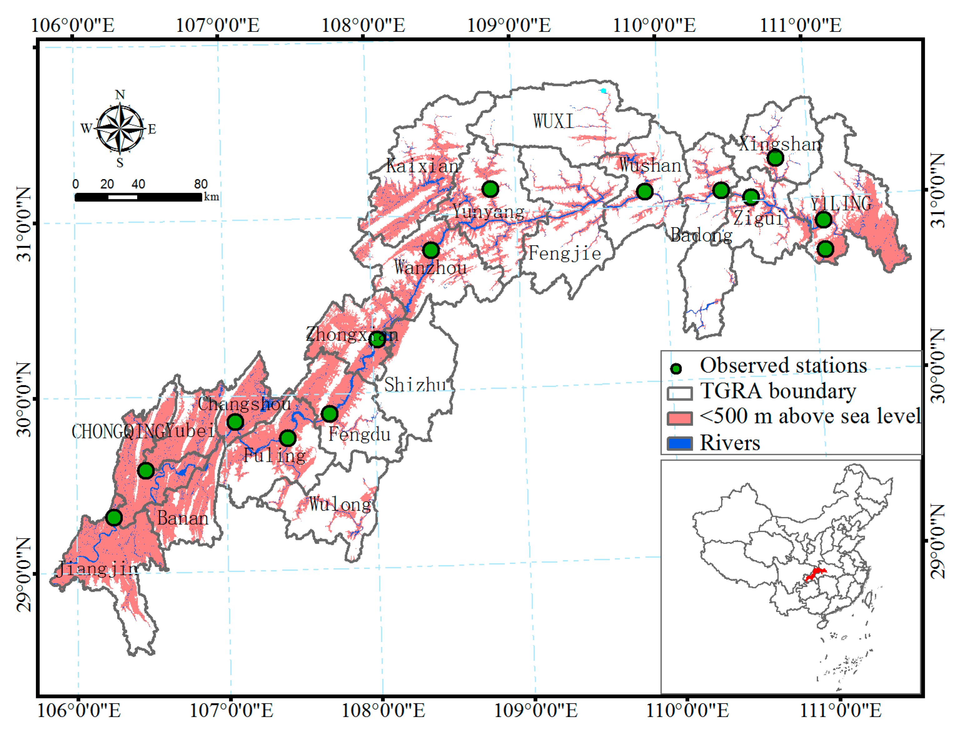
Figure 1. Location of study area and distribution of observed stations.
Sustainability 11 07206 g001
Figure 2. Time series and change trends of the station (observed) meteorological factors during 1973–2013. FD: annual fog days; RH: annual average air relative humidity: T: annual average temperature; PRE: annual precipitations. TFD, TRH, TT, and TPRE were the trends of FD, RH, T, PRE from 1973 to 2013, respectively, drawn as red lines. Means are the averages of annual values for the four factors from 1973 to 2013, drawn as red dotted lines.
Sustainability 11 07206 g002
Figure 3. Time series and change trends of the station (observed) meteorological factors in pre-dam (1973–1992), dam (1993–2009), and post-dam period (2010–2013). FD, T, RH, and PRE were the same as in Figure 2. The black line with black points represents the pre-dam period, the black line with red points represents the dam period, and the black line with blue points represents the post-dam period. Mean was multi-year average, and TFD, TRH, TT, and TPRE were the rate of trends.
Sustainability 11 07206 g003
Figure 4. Mann–Kendall (MK) test curves and accumulative anomalies curves of the station (observed) meteorological factors. a1), b1), c1), and d1) represent MK test results of the observed meteorological factors at the 95% confidence level; Uf are the statistics for the time series and Ub are the statistics for the inverse time series; a2), b2), c2), and d2) represent the accumulative anomalies curves. AAFD is accumulative anomalies of annual fog days, AAT is accumulative anomalies of annual average temperature, AARH is accumulative anomalies of annual average air relative humidity, and AAPRE is accumulative anomalies of annual precipitation.
Sustainability 11 07206 g004
Figure 5. Anomalies trends curves of the station (observed) meteorological factors in different periods. * documented that this parameter has passed the t-test at a 95% confidence level. The black line represents the period 1973–1995, the red line represents the period 1996–2013, the blue line represents the period 1996–2002, the magenta line represents the period 2003–2006, the olive line represents the period 2007–2010, and the navy line represents the period 2011–2013. AFD values are anomalies of FD, AT are anomalies of T, ARH are the respective anomalies of RH, and APRE are anomalies of PRE. Ta, Tb, Tb1, Tb2, Tb3 and Tb4 are the respective trends of AFD, AT, ARH, and APRE in the same period of the same color line, respectively.
Sustainability 11 07206 g005
Figure 6. Trends of the Station (observed) meteorological factors and NNR data (reanalysed) and the observed minus reanalysed (OMR) factors during 1973–2013. The black line indicates the annual anomalies of the observations, the red line indicates the annual anomalies of NNR, and the navy line indicates the annual anomalies of the OMR factors. Tob is the trend of the observations, Tnnr is the trend of the NNR, and TOMR is the trend of the OMR factors.
Sustainability 11 07206 g006
Figure 7. Land use/cover change (LUCC) from 1990 to 2010. Frt: forestry land, Agr: agricultural land, Wtr: water, Urb: urban-built land, Bal: bare land, A/F: area ratio of agricultural and forestry land, Vegetation: Frt and Agr.
Sustainability 11 07206 g007
Table 1. Correlation among station (observed) meteorological factors and NNR data (reanalyzed) in different periods.
Observed FactorsPeriodsFDTRHPRETnnrRHnnrPRWnnr
FD1973–20131−0.518 **0.705 **0.233−0.2270.557 **0.620 **
1973–19891−0.2620.665 **0.3250.3630.1800.591 *
1990–20101−0.596 **0.600 **−0.034−0.563 **0.598 **0.429
T1973–20131−0.659 **−0.2410.799 **−0.513 **−0.318 *
1973–19891−0.604 *−0.1370.633 **−0.153−0.013
1990–20101−0.624 **−0.2000.842 **−0.395−0.169
RH1973–201310.529 **−0.371 *0.635 **0.641 **
1973–198910.620 **−0.1440.550 *0.508 *
1990–201010.470 *−0.440 *0.476 *0.469 *
PRE1973–201310.0030.333 *0.476 **
1973–198910.1030.3710.475
1990–201010.1390.1790.428
Significance level: *, p < 0.05; **, p < 0.01. FD: annual fog days, T: annual average temperature, RH: annual average air relative humidity, PRE: annual precipitation; Tnnr: annual average reanalysed temperature, RHnnr: annual average reanalysed air relative humidity, PRWnnr: annual average reanalysed precipitable water.
Table 2. Correlation comparison among station (observed) meteorological factors and NNR (reanalyzed) data in different periods.
Observed Factors1973–20131973–19891990–2010
FDRH>PRWnnr>RHnnr>TRH>>PRWnnrRH, T, RHnnr>Tnnr
TTnnr>RH>FD,RHnnr>>PRWnnrTnnr>>RHTnnr>RH>FD
RHFD>T>PRWnnr>RHnnr>PRE>>TnnrFD>PRE>>T>>RHnnr>>PRWnnrT>FD>RHnnr>PRE, PRWnnr>Tnnr
PRERH>PRWnnr>>RHnnrRHRH
All abbreviations are the same as in Table 1. “>” represents correlation comparison at the 0.01 significance level. “>>” represents correlation comparison at the 0.05 significance level. “,” represents that the correlation coefficient difference is less than or equal to 0.05 at the same significance level.
Table 3. Correlation between station (observed) meteorological factors and area percentage of land use/cover changes (LUCC) from 1990 to 2010.
Observed FactorsUrbFrt AgrWtr A/F
FD−0.890 **−0.907 **0.892 **−0.746 **0.940 **
T0.511 *0.526 *−0.512 *0.394−0.563 **
RH−0.491 *−0.514 *0.490 *−0.3130.533 *
PRE−0.059−0.0690.070−0.0840.004
Urb, urban-built land; Frt, forestry land; Agr, agricultural land; Wtr, water; A/F, area ratio of agricultural and forestry land. Significance level and the other abbreviations are the same as in Table 1.
Table 4. Correlation between the observed minus reanalysed (OMR) meteorological factors and the area percentage of the LUCC from 1990 to 2010.
OMR FactorsUrbFrt AgrWtr A/F
OMR T−0.170−0.1540.152−0.1080.222
OMR RH0.464 *0.408−0.441 *0.566 **−0.388
Significance level and the other abbreviations are the same as in Table 3 and Table 4.