Comparing Transport Quality Perception among Different Travellers in European Cities through Co-Cluster Analysis


1
DIATI, Politecnico di Torino, C.so Duca degli Abruzzi 24, 10129 Torino, Italy
2
Department of Computer Science, University of Torino, C.so Svizzera 185, 10149 Torino, Italy
*
Author to whom correspondence should be addressed.
Sustainability 2019, 11(24), 7159; https://doi.org/10.3390/su11247159
Submission received: 20 October 2019
/
Revised: 10 December 2019
/
Accepted: 11 December 2019
/
Published: 13 December 2019
(This article belongs to the Section Sustainable Transportation)
Abstract
:The quality of the transport system offered at city level constitutes an important and challenging goal for society, for local authorities, and transport operators. Therefore, appropriate evaluation of travellers’ satisfaction is required to support service performance monitoring, benchmarking, and market analysis. This aspect implies the collection of satisfaction levels for different passengers’ groups, as it could provide interesting suggestions for identifying priority areas of action. To this end, an original study aimed at understanding the main aspects affecting the common view of satisfaction among different kinds of travellers at European level is presented in this paper. A specific survey investigating how travellers perceive the quality of their journey is proposed to people living in cities characterised by different sizes. Data are then analysed through a multi-view co-clustering algorithm, an innovative machine learning technique that highlights clusters of respondents grouped according to various categories of features. Such results could be used by local authorities and transport providers to understand the specific actions to be operated to improve the quality of transport service offered in a market segmentation dimension.
1. Introduction
The evaluation and assessment of the quality of transport offered is a challenging topic that has actracted many studies in the last years [1,2,3]. In addition, it is a crucial step in decisional processes, since policy makers and transport authorities are expected to assess the quality of all services. Clearly, an appropriate measure and analysis of satisfaction helps services performance monitoring, benchmarking, and market analysis. To this end, the collection of passengers’ satisfaction with a more specific interest in the needs of different user groups could provide interesting suggestions for service operators in order to identify priority areas of action. This operation could be performed in a city or a European dimension, appropriately considering different users’ groups and trying to go beyond a public transport level. So, the main goal should be, “the achievement of some general welfare objectives that justify public interventions (taxes and subsidies) on different transport services” [4].
Customer satisfaction surveys are usually necessary to investigate public transport travellers’ opinions. They can help in understanding which limitations could prevent potential users from choosing them for their journeys [5]. As a matter of fact, the competition with cars is strong, since these vehicles are—both as a matter of common knowledge and according to their users—appreciated thanks to their key determinants in the present busy lifestyle, such as comfort, flexibility, and speed [6]. Thus, a review of the literature of quality assessment of transport services shows that most of the papers focus mainly on public transport [7]. However, a more complete quality assessment exercise is expected to take into account other travel means, such as the active ones (bicycles, feet). Walking is “an inexpensive, emission-free, accessible for all form of mobility”, while “cycling is more and more considered as a mode of transport with high potential to address many urban mobility challenges, also due to the technological and societal developments” [8]. These active means can surely be seen more and more as a green and low impact alternative to widespread individual motorized vehicles. Policy makers are then required to investigate satisfaction levels also related to these kinds of travel means.
The actual performances of the different transport services provided are not the only factor affecting satisfaction ratings. Subjective conditions must be taken into account too, due to the often unequal characterisation of travellers’ needs and patterns. Their journeys are strongly related to their commitments and constraints, such as time and money. Moreover, people characterised by various socio-demographic variables, such as household composition, income level, profession, or car availability, could decide to use different travel modes for their displacements. Reference [9] provides an interesting overview of the literature related to salient characteristics of different travellers’ groups and the key factors affecting their perception. Specific approaches used to analyse various viewpoints could involve a market segmentation and how quality assessments vary in connection with travellers’ characteristics [10,11]. Reference [12] describes the innovative contribution proposed by the European project METPEX (A MEasurement Tool to determine the quality of the Passenger Experience). Its main aim is the provision of some innovative features able to answer the needs discussed previously, namely, aspects usually not investigated in most of the existing studies on quality measures. Firstly, all phases of the journey experience are considered, ranging from the pre-trip information acquisition process to the arrival at the destination. Moreover, satisfaction is investigated both for those people travelling on usual transit and for those using non-motorized transport means, such as bikes and feet, for their journey. A further challenging point is the interest in the specific viewpoints of particular groups of travellers, such as commuters, women, and physically challenged individuals. In this way, thanks to the indicators derived from the project, the policy makers are provided with a performing decision support tool essentially based on the feedback from different social groups.
As observed in [13], one of the problems with data acquired with personal and subjective surveys is the “subjective nature of such measurements, which consist of fuzzy and heterogeneous passenger assessments”. Limited literature can be found on this topic, since it seems to be a rather innovative and challenging issue. A recent work provides an interesting review on useful techniques for assessing the heterogeneity in travellers’ evaluation of public transport provision through the use of market segmentation techniques [3]. As detailed by the authors, various approaches coming from data mining and machine learning can be used to stratify the samples, such as “correspondence analysis, decision tree algorithms discriminant analysis, MNL [Multinomial Logit Model], and cluster analysis”. Moreover, various features can be taken into account in this stratification process: socio-economic attributes and travel attitudes [14], travel characteristics, trip satisfaction, trip practicality, familiarity and age [15], objective and subjective multimodal mobility levels, desired modal changes, and socio-demographic attributes [16]. Reference [13] showed that a possible solution could be the stratification of the sample of travellers according to their socio-economic characteristics or their travel attitude. According to the authors, the use of a data mining technique such as cluster analysis can be useful in transit service quality analysis, due to its ability in the segmentation process to, “reduce this heterogeneity, by segmenting the sample of passengers on groups that share some common characteristics, and that have more homogeneous perceptions about the service”.
The work presented in the current paper takes these previous contributions as a basis and expand them to a different level. Thanks to the rich dataset collected within the METPEX project, it is thus possible to apply an innovative unsupervised machine learning technique (called multi-view co-clustering) to different European test sites. Moreover, not only does the interest focus on public transport passengers, but also on usually poorly investigated user groups and means of transport. An interesting benchmarking analysis can be thus operated at European level, in order to understand where to concentrate specific actions necessary to improve the quality of transport services provided. The paper unfolds as follows. The next section explains how the technique applied works. Then, the background and the work behind the creation of the dataset are described, together with a deeper view of the variables used to define the features space. The following part deals with the presentation and the discussion of the results obtained with the co-clustering applied to two different features. The last section draws interesting conclusions and displays useful suggestions for future actions.
2. Materials and Methods
2.1. Clustering and Co-Clustering
Cluster analysis is a popular data mining technique used to partition objects into different groups (clusters), with the main goal of maximizing the homogeneity of the elements within each cluster and the heterogeneity between the various clusters. To clarify, while in the first case elements of the same cluster are expected to be as similar as possible, in the other one, elements from different clusters are requested to exhibit the highest dissimilarity [17]. Some works can be found in the literature that have applied this methodology in various ambits of transport engineering, such as transit quality evaluation [5,13] or tours classification [18]. Although some research has been carried out on the use of clustering to establish homogeneous groups of users with regards to service quality evaluation [11,13], to the authors’ knowledge this topic has not yet been proposed with a European benchmarking perspective. Moreover, in all these works the authors adopted standard k-means variants as the clustering method, but when data are heterogeneous and high-dimensional it fails in detecting high-quality and robust clusters [19].
To address the afore-mentioned issues, an innovative parameter-less machine learning approach based on multi-view co-clustering [20] is adopted in the current paper. Co-clustering [21] computes a partition of objects and a partition of features simultaneously, thus providing meaningful clusters of objects with a useful interpretation given by the grouping on features. It is worth noting that this approach is substantially different from clustering objects and features separately, since it adopts an objective function whose optimization takes into account both the object partition and the feature partition. Besides this, the problem of heterogonous (multi-view) data clustering is addressed. In this context, the same set of objects can be represented within different feature spaces or views (e.g., biographical data, census data, transport mode choice data). Clustering each feature space separately would result in different conflicting object partitions. On the other hand, processing all feature space as a whole would lead to a meaningless partition, since each feature space may fit a specific model, show properties, or be affected by certain problems such as noise, which might affect the other feature spaces in a different way. Moreover, the form of data may vary significantly from one space to another: transport mode information may be sparse, while biographical and census data are usually dense. The multi-view co-clustering task, instead, consists of clustering the set of objects according to multiple partitions on the spaces of features. Every feature space is partitioned according to a unique object partition, while the object partition is influenced by multiple feature space partitions simultaneously.
The multi-view co-clustering approach adopted here has another great advantage against classic clustering (e.g., k-means) and co-clustering (e.g., [21]) techniques: the algorithm automatically determines the number of clusters. This result is made possible by the use of the Goodman and Kruskal τ measure [22] as the objective function to be optimised. Given a partition of objects X and a set of partitions of features {Y1, Y2, …YN}, the Goodman–Kruskal τ estimates the association between X and {Y1, Y2, …YN} by measuring the proportional reduction of the error in predicting X, knowing or not {Y1, Y2, …YN}, and vice versa. Contrary to other optimization measures (such as the loss of mutual information [21]), the Goodman–Kruskal τ does not depend on the number of clusters. Thus, while in k-means clustering increasing the number of clusters always results in a better SSE (sum of squared errors), in this multi-view co-clustering schema this assumption is false, and the partitions providing the highest τ may have an arbitrary (usually small) number of clusters.
The co-clustering approach adopted for multi-view data is formulated as a multi-objective combinatorial optimisation problem which aims at optimising N + 1 objective functions. When evaluating the clustering of objects, the partition of objects is considered the dependent variable X (modelling the probability of the partitioning on objects), and the N partitions of the feature spaces are considered N independent variables {Y1, Y2, …YN} (each Yi models the probability of the partitioning of the i-th feature space). The objective function to be optimised is given by:
where is the error in predicting X without knowing {Y1, Y2, …YN} and is the expectation of the conditional error in predicting X when {Y1, Y2, …YN} are given.
During the evaluation of the partitions of features {Y1, Y2, …YN}, each Yi is considered a dependent variable and X an independent variable. The i-th objective function is then given by:
where and are defined as for . For the mathematical details and the complete description of the multi-view co-clustering algorithm, the user could refer to [20]. The source code of the algorithm is available online (https://github.com/rupensa/pycostar).
2.2. Experimental Framework and Dataset
The dataset at the basis of this paper came from the work done in the context of the METPEX project (A MEasurement Tool to determine the quality of the Passenger Experience, www.metpex.eu) [12]. The main goal of this FP7 European project was the implementation of a measurement tool for the passengers’ perceived quality of the whole journey experience, with a specific focus on some aspects usually less investigated in the existing studies. Hence, as explained previously, the special object of interest was the passenger experience across all phases of the journey. Moreover, special attention was devoted to non-motorized transport means (walk, bike) and to the opinions of particular groups of users, such as women, commuters, and physically challenged individuals [23].
A rather detailed questionnaire was formulated and proposed to the travellers of eight different European cities: Bucharest (Romania), Coventry (UK), Dublin (Ireland), Grevena (Greece), Rome (Italy), Valencia (Spain), Vilnius (Lithuania), and Stockholm (Sweden). Among the eight European cities investigated, only a selection of four was considered in the following according to the size of the test sites. These sites are different according to their dimensions, their location and, obviously, their mobility offer. However, the challenging aspect of the current study lay in the identification of common travellers’ behaviours in such different cities. With this aim, their selection was according to their number of inhabitants, in order to choose one city for each of the common definitions of settlement hierarchy: a small city, a medium-sized city, a large city, and a metropolis. More in detail, the number of inhabitants can be rounded to 30,000 for City A, to 500,000 for City B, to 800,000 for City C, and to 2,000,000 for City D. The surveying period began on 15 September 2014 and ran until 29 October 2014. It allowed the collection of 6360 responses through a variety of surveying protocols: paper-and-pencil, on-line web survey, navigator app, game app, and focus groups. More specific details on the project and the questionnaire implementation are provided in [24,25]. The questionnaire was made up of the following five parts:
- Baseline questions (BL): socio-demographic characteristics of the traveller, attributes of the last journey done, general opinions, and mood;
- Tier 1 quality questions (T1): five-point scale satisfaction ratings of 21 quality components related to the overall journey;
- Mode-specific questions (TM): five-point scale satisfaction ratings for questions specific to one of the travel means used by the traveller;
- User group-specific questions (UG): five-point scale satisfaction ratings for questions specific to one of the users groups the traveller falls in;
- Tier 2 quality questions (T2): five-point scale satisfaction rating questions for an in-depth assessment of a randomly selected T1 quality component.
According to the formulation of the questionnaire, all interviewees had to complete section BL and T1, so the related questions collected the greatest number of answers. Consequently, the analysis presented in this paper concentrates on variables coming from these two parts of the dataset. Deeper attention must be devoted to the rating provided for the 21 quality components in the T1 section. As can be imagined, not all 21 questions were always answered by each traveller, so a cleaning procedure was necessary: an observation was discarded when fewer than 16 of them had not been evaluated. When, instead, an observation passed the previous cleaning step, but some questions were not rated by a traveller, specific values were assigned by default. Firstly, the mean value of all the ratings for a specific indicator in a specific city was derived. Then, all the evaluations effectively provided in the T1 section by the traveller under investigation were considered and their mean value was computed. The default values were then assigned to the missing T1 questions as the mean value of the two contributions described herein. In this way, all 21 features of the dataset referring to the indicators were different from 0.
After the cleaning operation described, 103 elements were found for City A, 447 for City B, 552 for City C, and 296 for City D. Table 1 provides the partitions among the different features (gender, age, and working status) derived from part BL of the questionnaire for the four test sites. Male and female travellers had different splits in each city, with a significant majority of women in City D and a rather uniform distribution in the others. Age groups did not collect the same number of occurrences in all four datasets, depending on the sampling plan and the responses rates. For example, City A was the only instance of a category that included half of the interviewees (18–24). In the other datasets, this age group was responsible for a great number of answers too, but the distribution among the different classes was more balanced.
At first glance, the last feature of Table 1(working status) shows a category which predominated strongly and that varied according to the test site. In City A this was certainly correlated with the age group discussion presented previously, since 45.6% of respondents were classified as students, while 16.5% and 14.6% were self-employed and full-time workers, respectively. Respondents in City B were split into two main working categories, full-time workers (44.3%) and students (21.7%), rather similarly to City C, where the percentages were almost equal (33.8% and 32.0%, respectively). However, in this site other categories were also well represented, such as part-time workers (11.1%) and working students (9.8%). In City D, the great majority of interviewees fell into the full-time workers class (55.1%). Two other working statuses were rather well represented in this city: students (13.9%) and pensioners (11.1%). An objective of this paper was to see if the different partitions among the various classes influenced the results of the analysis or if it was possible to obtain interesting and repeatable results despite the variations in the dimension of the classes considered in the four cities.
The previous three features are more linked to socioeconomics and personal attributes of the travellers, since they came from the BL part of the questionnaire. A further one was added, which took into account the mobility attitude: the means of transport used by the traveller in the journey investigated was thus the next feature considered. Ten main classes were defined: bicycle, demand responsive, mobility vehicle, pedestrian, private vehicle, public transport on rail, public transport on road, tram, underground, waterborne. Obviously, the interviewee could have used only one or a combination of them for the journey considered.
Table 2 provides the distribution of the modes for the four cities selected. For this analysis, the ten modes were grouped into five main categories: IM stands for individual means (private vehicle), PT is transit modes (public transport on rail, on road, tram, underground, and waterborne), BI refers to bikes, WA to walking, and OT labels the remaining means (demand responsive and mobility vehicle). The rows in italics show the totals when one, two, three, and four modes were used in the journey, irrespective of their combinations. At first view, all cities demonstrated a prevailing trend in the combined use of means except for City C, where monomodality characterised 52.5% of journeys analysed. The greatest contribution to this result was given by the class PT (39.1% of cases), which included all kinds of public transport and their combinations. As shown in the first five rows of Error! Reference source not found., the predominance of transit as a unique mode held in the other cities too, apart from City A, where the highest value was instead reached by individual means (IM).
In a certain way, the importance of public transport in the travellers’ mobility was a result tainted by one of the objectives of the questionnaire, which focused mainly on transit users’ satisfaction. However, as said previously, the interest in both active and other kinds of means was a specific task of the research project and so other relevant aspects were observed in the dataset. City A showed the most multimodal attitude, as demonstrated by the value 87.3% as the sum of 84.4% and 2.9%. Moreover, the highest percentage in Table 2 was found in this city for PT WA (71.84%). The dimensions of the test site were certainly responsible for these behaviours, as this city was the smallest of the four. A citizen of this city probably faces a narrower offer of means of transport and has to combine more modes to reach their destination. Similarly, the monomodality attitude of City C shows the profile of a city with an efficient transit network, allowing many users to travel all around. The rows of Table 2 referring to the combinations of three or four modes show interesting results too: the highest values were reached for City B (12.8%) with the majority of occurrences for the case IM PT WA. Again, an explanation could be the dimension and the profile of the test site. This city is probably characterised by a narrow public transport network with private means being necessary to reach intermodal interchanges (stations, park and ride points).
In part T1 of the questionnaire, travellers were asked to rate quality issues: the specific questions are listed in the second column of Table 3. These 21 indicators came both from the literature on the topic, such as [26] or [27], and from innovative contributions to the field [4,24]. Concepts usually not considered in quality evaluation, such as design (T1_1, T1_2, T1_3, T1_12, T1_20) and intermodality (T1_5, T1_15), were introduced. Then, the core of the METPEX project—that is, the whole passenger experience—was investigated and evaluated through questions such as T1_4 (meeting of mobility needs) and T1_6 (respect of travellers’ rights). Users not usually considered, such as those with additional needs and those using motorised vehicles, were instead taken into account thanks to T1_7 and T1_16.
Some considerations arose looking at the mean values derived for the indicators in the four test sites (last columns of Table 3). The multimodal City A collected the overall lowest value (3.1), while the monomodal City C had the highest (3.6). The already observed attitudes could influence these result as, for example, the T1_15 indicator evaluating the support for intermodal travels showed the lowest value among the 21 questions for City A (2.3). Overall, it is possible to notice some similarities between the four test sites, even when each of them showed different trends in the ratings. In almost all the cities travellers were not as satisfied with indicators as they could be, for example, the already cited T1_15 or T1_21. Similarly, aspects such as safety and security (T1_14) reached rather high ratings irrespective of the test site.
In the following, the personal features analysed here are merged with the journey characteristics and the values of the indicators to create the dataset in which multi-view co-clustering was applied. The information presented in this section seems to sketch a specific profile of travellers and the mobility offered in each city certainly plays an important role. The goal was to find users’ behaviours and characteristics that were repeated despite the test site considered. At the same time, it is interesting to see if the indicator ratings helped in the definition of these clusters and showed specific trends in each of them. Useful suggestions could thus be given to policy makers to ameliorate the transport services provision and to highlight positive aspects of the present mobility offer.
3. Results and Discussion
The dataset described in the previous section, made up of five features (gender, age range, working status, means used for the journey, and satisfaction ratings), was analysed through the multi-view co-clustering method presented in Section 2.1. Data collected in each test site were considered separately, in order to see how many and which clusters of users originated. The ability of this technique to determine the proper number of clusters that could be found in the dataset by itself, without any input from outside, allows the data “to talk” and to identify intrinsic similarities.
According to the procedure followed, a binary value of 0 or 1 was assigned to the variables of Table 1 and to each of the features representing one of the ten modes considered. Obviously, in this latter case, more than one value 1 could be assigned for each traveller if they had used different modes in the journey considered. The pre-processing procedure applied to the 21 T1 quality indicators has already been explained in the previous section: this was necessary since, during the data collection, a 0 value was assigned when an indicator was not rated by the traveller. However, the co-clustering approach implemented would see this 0 as a rating and not as a missing value, producing biased results. Moreover, each one of the 21 quality indicators was split into three binary features to improve the efficiency of the algorithm. According to the value of the indicator, it could be classified as ‘low’ if it was lower or equal to 2.25, ‘mean’ if it belonged to the interval 2.25–3.75, or ‘high’ if it was higher than or equal to 3.75. Thus, 63 (3 x 21) binary features were derived from the 21 indicators of part T1 and were used in the analysis.
Two different approaches are proposed in this paper. In the first case, only the socioeconomic and travel-related variables were used to identify the clusters (Clus1 in the following), while in the second one the quality indicator binary features were added too (Clus2 in the following). The results obtained in both cases are presented, seeing how the variables available behaved in the clusters derived by the algorithm. Once the various clusters were identified, a specific analysis was proposed, investigating the characteristics of the travellers belonging to them, as shown Table 4 and Table 5 for Clus1 and Clus2, respectively. Different groups of users dominated in each city and it is interesting to notice that very similar features were found when comparing the test sites. Figure 1 and Figure 2 present the partition of travellers in each location through pie charts, while specific icons visually represent the characteristics of the different clusters.
In Table 4 and Table 5, the percentages of elements found are firstly reported for each cluster and in each test site. Then, the features collecting a relevant number of occurrences were taken into account, after having grouped them in the main variables according to the second column of Table 1. If a feature characterised a great majority of elements of a specific cluster, an ‘x’ sign is shown in the corresponding column in Table 4 and Table 5. A similar procedure was applied for the variable “transport modes”, where the ten means were grouped in the five main categories defined in the previous section. If a variable of those defined in the third column of Table 1 is not found in Table 4 or Table 5, it means that it did not have a relevant influence in the clusters. The last three columns in the tables refer to the T1 indicator trends characterising each cluster. These trends were available for both Clus1 and Clus2, since each observation was assigned to a specific group after the co-clustering operation. In this way, all the ratings of the 21 elements of Table 3, which correspond to all travellers belonging to a cluster, were averaged, and this final value is reported in the column named “mean”. Moreover, special interest was given to the indicators reaching the highest and the lowest voting in each cluster and each city (”min” and “max” columns) in order to find potential similarities among both the test sites and the identified groups.
3.1. Results for Clus1
Table 4 and Figure 1 show the clusters found with the procedure Clus1, which used four features as variables for the co-clustering (gender, age, working status, and means). At first glance, three clusters were identified in City A and City B, while only City C and City D held elements belonging to a fourth group too. Looking at the common characteristics, specific classes of users seemed to come out from the co-clustering analysis. In all test sites, clusters of type “_1” refer to young students, while aged people not working were assigned to clusters labelled with “_3” in City A and with “_4” in City C and D. In all these cases, the means of transport mainly used were a combination of transit and walking. These were also the modes which characterised Clus1B_2, Clus1C_3, and Clus1D_3 and that were common for young or adult workers. However, there were some clusters in which travellers belonging to this working status used other means for their journey: in fact, individual motorised modes were combined with public transport in Clus1B_3 and with walking in Clus1A_2. Bicycles characterised two small clusters: in City C, 5% of interviewees used these combined with walking, while in City D they were joined with individual motorised modes and transit in 1% of cases. Working status for these instances was workers and students in the former case and only workers in the latter one.
Some interesting results are shown in the last three columns of Table 4 for all cities. As already explained, at this stage, the ratings provided by the users were not included among the variables of the co-clustering process. Thus, these results were only influenced by the personal characteristics and the mobility attitude of the travellers. In City A, indicators referring to specific aspects of public transport, such as ticketing and pre-trip information (T_17 and T_11), reached high values among the working and not working user groups. However, the level of information provided decreases during the journey, as stated by the low rating of T1_10 in Clus1A_3. The recognition of the needs of motorised vehicle users (T1_16) was placed in the “min” column for Clus1A_3, which was popular for workers using this kind of means for their journey. This aspect could be certainly challenging for policy makers in this city. It is also interesting to notice that an indicator related to multimodality, T1_15, was not appreciated (column “min”) by the students’ cluster, highlighting some limitations of the city in fulfilling these needs.
Some considerations about multimodality and proper interaction among different means of transport are shown in the results of City B too. As already stated previously, this test site was the one reporting the highest occurrences for the case of journeys where three modes were used in combination (12.8% in Table 2). The indicator related to the support for intermodal travel (T1_15) reached rather low values in ClusB1_2 and ClusB1_3. However, an overall comparison of the indicators reported in Table 4 for this city showed some recurring trends, as deduced from the repetitions found in both the “max” and the “min” cells. For example, travellers felt that their mobility needs (T1_4) and their passenger’s rights were respected (T1_6), as revealed by the high ratings assigned to these indicators in all clusters. On the other hand, none of the user groups thought that value for money of services was good (T1_21).
Four different clusters were detected in City C with the co-clustering technique. While the first three were rather similar to those in City A and City B, a new one was found, which was characterised by young and adult workers travelling by active means. The already cited monomodality attitude of this test site can be confirmed by the absence of indicators T1_5 and T1_15 among those in the last columns in Table 4. Highlighting the elements reaching the highest and lowest rating values in the clusters is useful to understand the aspects to be addressed by specific actions of policy makers. Travellers of three clusters found that their safety and security while travelling were good (T1_14) and that transport availability was adequate for their needs (T1_19). A common feature in all clusters was the feeling about the way the city addresses the needs of motorised vehicle users: in fact, T1_16 fell in the “min” cells in all cases, which were characterised by the use of transit or active means. This result could be interpreted as the fact that potential motorised vehicle users do not change their mode choice, migrating to individual motorised means, since they think it is not worth doing it.
In City D, as in City C too, four classes were identified. Any indicator gained the highest satisfaction in all clusters, but it is interesting to observe if features appreciation was common among the different classes. Three clusters provided high ratings to the ticketing purchasing ease (T1_17) and low ones to the accessibility for travellers with additional needs (T1_7). The fact that these three user groups were those revealing the greatest transit use attitude could provide useful hints to stakeholders and policy makers on which are the positive and negative points in the public transport provision. Common features were found in Clus1D_3 and Clus1D_4. In both cases, T1_6, which referred to the respect of passenger rights, was found in the “max” cells, while the “min” rows contained the indicator T1_15, showing that those users were not satisfied with the intermodal travel support provided by the city. Analogously, in cluster Clusd1D_2, which was characterised by a small number of workers combining transit, bicycle, and individual motorised means for their journey, a high opinion on this topic was not observed, mainly because of the design aspect of main terminals (T1_18 in ‘min’ column). This aspect could be an interesting point of view, since this group of travellers effectively combined these means in their journey. However, this wass the only case where indicator T1_21 was placed in the “max” column. On the whole, all these results demonstrate that different kind of travellers have different needs and quality perceptions, and so specific initiatives should be promoted.
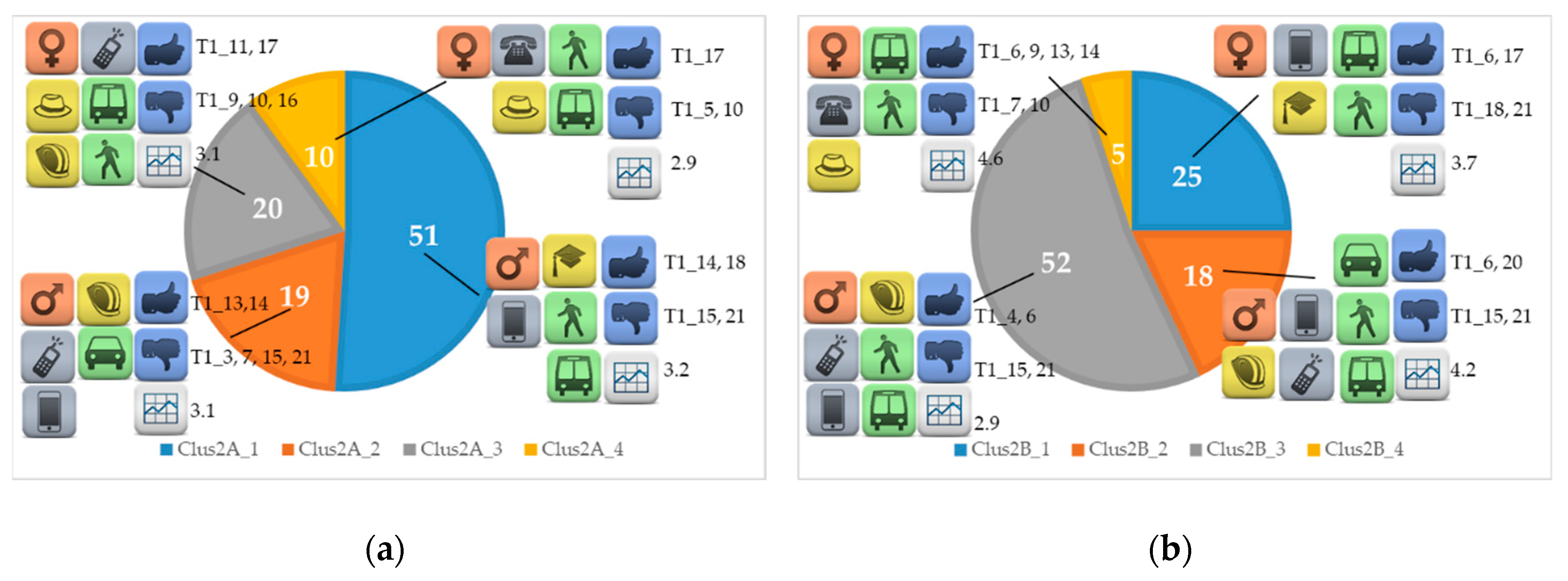
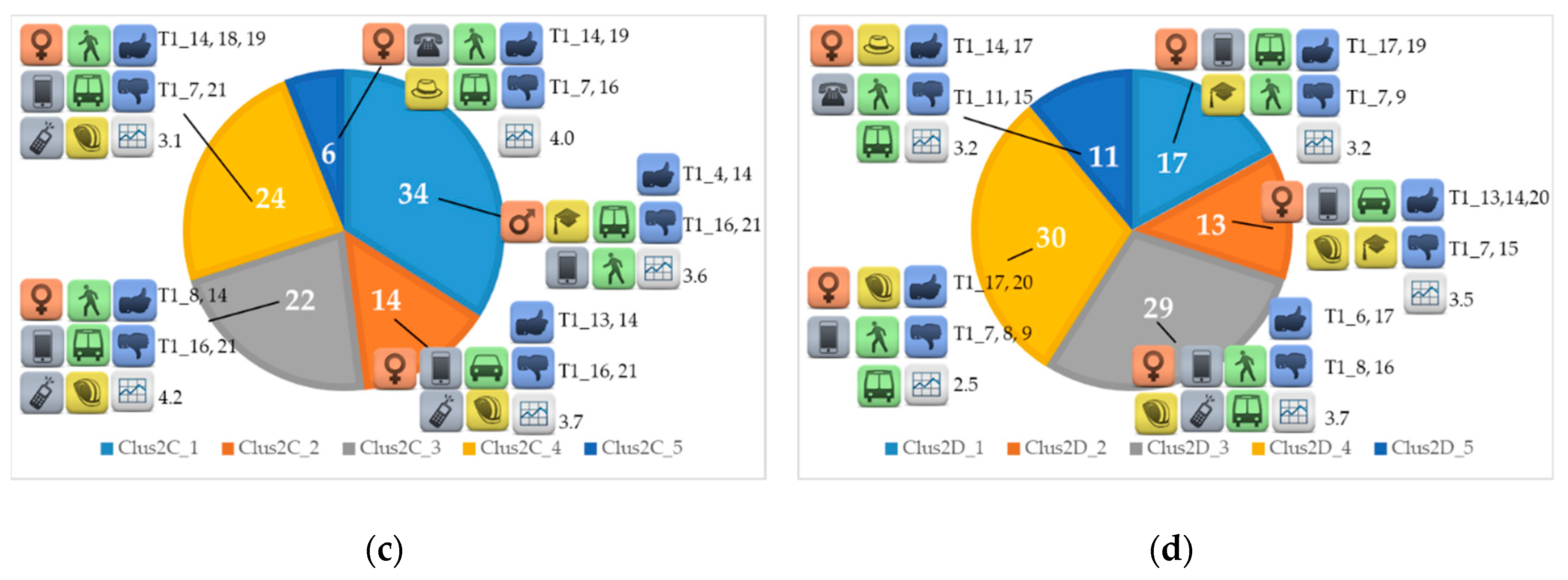
3.2. Results for Clus2
The results obtained considering socioeconomics and travel-related variables with the addition of quality indicators binary features, namely the Clus2 procedure, are then presented in Table 5 and in Figure 2. In this case, the multi-view co-clustering technique was applied, using all five variables described in the previous section: gender, age, working status, means, and T1 indicators ratings translated to a binary scale. In each test site, the number of clusters found was increased by one if compared to the results of Clus1. The introduction of the ratings as variables helped in the definition of more homogenous groups of users among all cities. It is possible to see that clusters of type “_1” refer, as in the Clus1 case, to young students, while aged people not working are now found in all test sites and are labelled with “_4” in City A and B with “_5” in City C and D. As previously, in all these classes travellers used both transit and walking in their journey. A new kind of user is now identified—young people and adults moving only with individual motorised means (Clus2A_2, Clus2C_2, and Clus2D_2) or using them in combination with transit and walking (only in Clus2B_2). As for the Clus1 case, groups of people travelling with public transport and walking were found in all cities, but the introduction of the ratings as a variable led to a further partition. In fact, in City C and D, two different clusters showed workers moving by transit: the main difference was the mean value of ratings. As could be seen in the “mean” column in Table 5, Clus2C_3 and Clus2D_3 had higher values (4.2 and 3.7) compared to Clus2C_4 and Clus2D_4 (3.1 and 2.5).
Some useful hints and results could be derived by looking at the last two columns of Table 5, which enrich the observations already detailed for the case Clus1. As a matter of fact, with the introduction of the ratings as variables, other elements could be common to the observations assigned to each cluster in the different test sites. For example, repeated indicators were found in the first two and in the last two user groups in City A. T1_14 was placed in the “max” column for both ClusA2_1 and Clus2A_2, while T1_15 and T1_21 were in the “min” one for the same clusters. Similar behaviour was seen for T1_17 and T1_10 in Clus2A_3 and Clus2A_4. Moreover, a discussion on multimodality could be operated. As already said for Clus1, indicators related to multimodality were not appreciated by all the user groups considered, highlighting some limitations of the city in fulfilling these needs: three of the four clusters in City A showed T1_5 and T1_15 in the “min” column.
The introduction of ratings as variables in the co-clustering procedure helped give a clearer definition of the class of aged not-working travellers in City B, too. This city was the only test site where this cluster was not found in Clus1, showing that this group of travellers provided common T1 indicator ratings. For example, elderly people are surely more sensitive to the overall accessibility for travellers with additional needs, as this could be them. T1_7 dealt with this aspect and it fell in the “min” column for the cited Clus2B_4 cluster, while it was not found in Table 4 in the same test site. Other aspects based mainly on public transport provision were indicated in that comparison. As can be seen in Table 5, this group of travellers provided high ratings to indicators not revealed previously, such as T1_9, T1_13, and T1_14, which accounted for the receptiveness of staff, ride quality, and safety and security. These are surely useful feedback for the transport service provider of this city, both on those aspects that could be ameliorated and on those well developed. An interesting point is a wide difference between the highest and the lowest mean value found for T1 indicators in City B. As can be seen in the table in the rows corresponding to that test site, the maximum (4.6) was reached for Clus2B_4, while the minimum was reached(2.9) for Clus2B_3. The fact that the modes used by both groups were the same (PT and WA) provides interesting hints on how different kinds of travellers (pensioners and workers, in this case) have different perceptions of service quality, and which are those aspects that should be improved to increase the satisfaction level.
The analysis of the results found for the City C showed, as already said, the introduction of a new cluster and some differences if compared to those obtained with the Clus1 procedure. Bikers were no more present in a consistent number in any of the four classes, while a collection of individual motorized means users originated. Moreover, the cluster that represented transit travellers and pedestrians in Table 4 (Clus1C_3) was now split into two groups characterised by a different mean value of T1 indicators, maximum in one case, minimum in the other one. Common elements were found in the last two columns of Table 5 for those travellers walking and using public transport for their journeys, mainly concerning unsatisfying aspects. In the “min” column T1_21, T1_16, and T1_7 were repeated, while T1_14 was seen in the “max” one for all the rows of City C. Other aspects reaching high values changed across the different kind of user groups. For example, young students and pensioners (aged not working) were pleased with the transport system provision (T1_4 and T1_19), while young and adult workers, probably commuters, appreciated the provision of information on arrivals and departures and the punctuality (time the journey took was as promised).
Five clusters were found also in City D, with a test site profile similar to that of City C, with the loss of the bikers cluster and the creation of the two levels of transit satisfaction. However, elements derived from the T1 indicators analysis recalled those found in Clus1, such as the repeated presence of T1_17, T1_7, and T1_15. At the same time, interesting aspects emerged as the non-satisfying provision of information on arrivals and departures reported by workers travelling by transit. Moreover, common features were found between people using different modes for their journey in Table 5, too. For example, users belonging to both Clus2D_2 and Clus2D_3 thought that their safety and security when travelling was good (T1_14). Other aspects linked to the quality of transit service provided could be highlighted, such as the proper respect of passenger rights (T1_6 in Clus2D_3), the vehicle design suitable for the workers’ needs (T1_20 in Clus2D_4), the lack of receptiveness of the public transport staff to the travellers’ needs (T1_9 in Clus2D_1), and the low quality of pre-trip information (T1_11 in Clus2D_5). All these contributions provide useful information on those topics that need to be ameliorated in the test site to provide an efficient and satisfying transport service offer.
4. Conclusions
In this study, an innovative analysis of the transport services quality at a European level was proposed. One of the main goals was the comprehension of those aspects affecting the common view of satisfaction among different kinds of travellers. In this way, it was possible to understand where to concentrate specific actions necessary to improve the quality of transport services provided in a market segmentation dimension. Data collected through a survey presented in different European cities were analysed thanks to multi-view co-clustering. The fundamental advantage of this technique was, as explained in the second section, its ability in finding proper clusters in itself. The same procedures presented in this paper were conducted with a traditional k-means clustering algorithm, too. The results obtained were not shown here because it is out of the scope of this paper, but they are available from the authors upon request. However, if the k-means algorithm is asked to find the same number of clusters derived with the co-clustering, a less clear and well-defined partition between the different classes of travellers is derived.
On the whole, the features presented in Table 1, together with their percentages, certainly had a strong influence on the creation of the various groups of travellers. For example, the combination of working status and age, i.e., two features of the five used in the definition of the dataset, is supposed to affect the definition of clusters aggreagating young people or those collecting the elderly not working. An explanation could be found looking at values in Table 1 for the classes 18–24 and “students”, which usually overlapped, and which were rather numerous in all cities. The same overlap held for the groups 65–74 and “pensioner”, which instead characterised a lower number of interviews. The technique applied was able to identify this category of travellers despite its small dimensions, probably thanks to other elements common to them, such as the ratings provided. Similar observations arise looking at the row of Table 2 referring to IM. As an example, only City B did not show a high tendency to the use of individual modes, but co-clustering identified a class of full-time workers using private vehicles in all cities, only with the addition of the T1 indicators ratings as features (Clus2 approach). Thus, as previously, other components had great influence and prevented the creation of that specific group of travellers.
After having showed, with the use of a machine learning technique, the existence of well-defined classes of users, the comparison of the different clusters originating in each city opened a window on interesting suggestions to policy makers and stakeholders. At the same time, matching the results of those groups among the various test sites made it possible to derive useful suggestions for mobility actions at European level, once common elements were found. A negative perception of value for money of services affected many travellers, as derived by the low rating always assigned to the corresponding indicator, except for City D. An accessibility not fully adequate for travellers with additional needs was another aspect characterising the journey of at least one users group in each city. The possibility of using different forms of transport during the same trip was not that satisfactory, according to the respondents, in almost all test sites (excluding City C). While this could be rather reasonable in the smallest cities, such a facet is expected to be investigated and mitigated in City D. As already discussed, safety and security in cities are usually challenging objectives that are not always easy to reach. However, the high ratings associated with the related indicator (and found in all clusters and in all test sites) show that proper actions have been made at European level. A further result highlighted by this study confirmed the good actions undertaken by EU in the field of passenger rights. This is, in fact, one of the few areas where citizens are protected by a full set of passenger rights, irrespective of the means used.
As explained in the introduction, most of the studies on these topics in the literature focus on the quality of public transport services. However, thanks to the contribution of METPEX project in the development of indicators wishing to investigate the satisfaction of all kinds of travellers, interesting suggestions were derived for individual motorised vehicles and bicyclist, too. As shown in the paper, the two approaches presented were able to identify clusters with respondents using individual modes for their journeys, separating those travelling by bike or by motorised means, despite their low numbers. According to the results, these users were characterised by similar perceptions: in fact, both kinds of travellers assigned good ratings to the ride quality, to the travel safety and security, and to the design of the chosen vehicles, as obviously they were owned by them. Negative aspects among people using motorised vehicles were, instead, the negative perception of value for money of service, the accessibility for travellers with additional needs, and the unsatisfying provision for intermodal travel support. This last feature could be surely one of the motivations behind that specific mode choice and proper actions should be done to push to a modal change.
The results given by this work provide interesting insights into the travellers’ perception of their journey, which could be very heterogeneous if looked at from a more global perspective. However, a procedure like the one proposed aims to find common elements to define similar classes of users, collecting and highlighting the needs and the opinions of specific groups of travellers. Many players could be interested in such applications and results, at European, regional, or city level. A joint work of transport planners, policy makers, and transport services providers could, indeed, delineate users’ profiles and detail specific and personalised strategies addressing the proper actions to ameliorate the whole transport system provision.
Author Contributions
Conceptualization, M.P.; data curation, M.P.; formal analysis, M.P.; methodology, M.P. and R.G.P.; software, R.G.P.; validation, M.P.; writing—original draft preparation, M.P. and R.G.P.
Funding
This research received no external funding.
Acknowledgments
The dataset analysed in this article was collected within the European project METPEX (A MEasurement Tool to determine the quality of the Passenger Experience, www.metpex.eu), which has received funding from the European Union’s Seventh Framework Programme under grant agreement No. 314354 and lasted from 1 November 2012 to 31 October 2015.
Conflicts of Interest
The authors declare no conflict of interest.
References
- Chica-Olmo, J.; Gachs-Sánchez, H.; Lizarraga, C. Route effect on the perception of public transport services quality. Transp. Policy 2018, 67, 40–48. [Google Scholar] [CrossRef] [Green Version]
- Deb, S.; Ali Ahmed, M. Determining the service quality of the city bus service based on users’ perceptions and expectations. Travel Behav. Soc. 2018, 12, 1–10. [Google Scholar] [CrossRef]
- Abenoza, R.F.; Cats, O.; Susilo, Y.O. Travel satisfaction with public transport: Determinants, user classes, regional disparities and their evolution. Transp. Res. Part A Policy Pract. 2017, 95, 64–84. [Google Scholar] [CrossRef] [Green Version]
- Diana, M.; Duarte, A.; Pirra, M. Transport Quality Profiles of European Cities Based on a Multidimensional Set of Satisfaction Ratings Indicators. Transp. Res. Rec. J. Transp. Res. Board 2017, 2643, 84–92. [Google Scholar] [CrossRef] [Green Version]
- de Oña, R.; López, G.; de los Rios, F.J.; de Oña, J. Cluster Analysis for Diminishing Heterogeneous Opinions of Service Quality Public Transport Passengers. Procedia Soc. Behav. Sci. 2014, 162, 459–466. [Google Scholar] [CrossRef] [Green Version]
- Bergstad, C.J.; Gamble, A.; Hagman, O.; Polk, M.; Gärling, T.; Olsson, L.E. Affective–symbolic and instrumental–independence psychological motives mediating effects of socio-demographic variables on daily car use. J. Transp. Geogr. 2011, 19, 33–38. [Google Scholar] [CrossRef]
- de Oña, J.; de Oña, R. Quality of Service in Public Transport Based on Customer Satisfaction Surveys: A Review and Assessment of Methodological Approaches. Transp. Sci. 2015, 49, 605–622. [Google Scholar] [CrossRef]
- EU Commission. A European Strategy for Low-Emission Mobility; Communication from the Commission to the European Parliament, the Council, the European economic and social Committee and the Committee of the Regions; European Commission: Brussels, Belgium, 2016. [Google Scholar]
- Susilo, Y.O.; Cats, O. Exploring key determinants of travel satisfaction for multi-modal trips by different traveler groups. Transp. Res. Part A Policy Pract. 2014, 67, 366–380. [Google Scholar] [CrossRef]
- Dell’Olio, L.; Ibeas, A.; Cecin, P. Modelling user perception of bus transit quality. Transp. Policy 2010, 17, 388–397. [Google Scholar] [CrossRef]
- Bordagaray, M.; Dell’Olio, L.; Ibeas, A.; Cecín, P. Modelling user perception of bus transit quality considering user and service heterogeneity. Transp. A Transp. Sci. 2014, 10, 705–721. [Google Scholar] [CrossRef]
- Woodcock, A.; Susilo, Y.; Diana, M.; Abenoza, R.; Pirra, M.; Tovey, M. Measuring Mobility and Transport Services: The METPEX Project. Adv. Hum. Asp. Transp. 2018, 597. [Google Scholar]
- de Oña, J.; de Oña, R.; López, G. Transit service quality analysis using cluster analysis and decision trees: A step forward to personalized marketing in public transportation. Transportation 2016, 43, 725–747. [Google Scholar] [CrossRef]
- Shiftan, Y.; Outwater, M.L.; Zhou, Y. Transit market research using structural equation modeling and attitudinal market segmentation. Transp. Policy 2008, 15, 186–195. [Google Scholar] [CrossRef]
- Jacques, C.; Manaugh, K.; El-Geneidy, A.M. Rescuing the captive [mode] user: An alternative approach to transport market segmentation. Transportation 2013, 40, 625–645. [Google Scholar] [CrossRef]
- Diana, M.; Mokhtarian, P.L. Grouping travelers on the basis of their different car and transit levels of use. Transportation 2009, 36, 455–467. [Google Scholar] [CrossRef]
- Tan, P.-N.; Steinbach, M.; Kumar, V. Introduction to Data Mining; Pearson Addison Wesley: Boston, MA, USA, 2005; ISBN 0321321367. [Google Scholar]
- Pirra, M.; Diana, M. Classification of Tours in the U.S. National Household Travel Survey through Clustering Techniques. J. Transp. Eng. 2016, 142, 1–13. [Google Scholar] [CrossRef] [Green Version]
- Sun, J.; Lu, J.; Xu, T.; Bi, J. Multi-view sparse co-clustering via proximal alternating linearized minimization. In Proceedings of the 32nd International Conference on Machine Learning, Lille, France, 6–11 July 2015; pp. 757–766. [Google Scholar]
- Ienco, D.; Robardet, C.; Pensa, R.G.; Meo, R. Parameter-less co-clustering for star-structured heterogeneous data. Data Min. Knowl. Discov. 2013, 26, 217–254. [Google Scholar] [CrossRef] [Green Version]
- Dhillon, I.S.; Mallela, S.; Modha, D.S. Information-theoretic co-clustering. In Proceedings of the ninth ACM SIGKDD International Conference on Knowledge Discovery and Data Mining—KDD ’03, Washington, DC, USA, 24–27 August 2003; ACM Press: New York, NY, USA, 2003; p. 89. [Google Scholar]
- Goodman, L.A.; Kruskal, W.H. Measures of association for cross classification. J. Am. Stat. Assoc. 1954, 49, 732–764. [Google Scholar]
- Pirra, M.; Diana, M.; Castro, A. Information provision in public transport: Indicators and benchmarking across europe. In Proceedings of the Transport Infrastructure and Systems—Proceedings of the AIIT International Congress on Transport Infrastructure and Systems, TIS 2017, Rome, Italy, 10–12 April 2017; pp. 681–688. [Google Scholar]
- Diana, M.; Pirra, M.; Castro, A.; Duarte, A.; Brangeon, V.; Di Majo, C.; Herrero, D.; Hrin, G.R.; Woodcock, A. Development of an Integrated Set of Indicators to Measure the Quality of the Whole Traveller Experience. Transp. Res. Procedia 2016, 14, 1164–1173. [Google Scholar] [CrossRef] [Green Version]
- Susilo, Y.O.; Woodcock, A.; Liotopoulos, F.; Duarte, A.; Osmond, J.; Abenoza, R.F.; Anghel, L.E.; Herrero, D.; Fornari, F.; Tolio, V.; et al. Deploying traditional and smartphone app survey methods in measuring door-to-door travel satisfaction in eight European cities. Transp. Res. Procedia 2017, 25, 2262–2280. [Google Scholar] [CrossRef] [Green Version]
- de Oña, R.; Eboli, L.; Mazzulla, G. Monitoring Changes in Transit Service Quality over Time. Procedia Soc. Behav. Sci. 2014, 111, 974–983. [Google Scholar] [CrossRef] [Green Version]
- Tyrinopoulos, Y.; Aifadopoulou, G. A complete methodology for the quality control of passenger services in the public transport business. Eur. Transp. 2008, 38, 1–16. [Google Scholar]
Figure 1.
Graphical representation of the characteristics of the clusters obtained with the approach Clus1 for: (a) city A; (b) city B; (c) city C; (d) city D.
Figure 1.
Graphical representation of the characteristics of the clusters obtained with the approach Clus1 for: (a) city A; (b) city B; (c) city C; (d) city D.
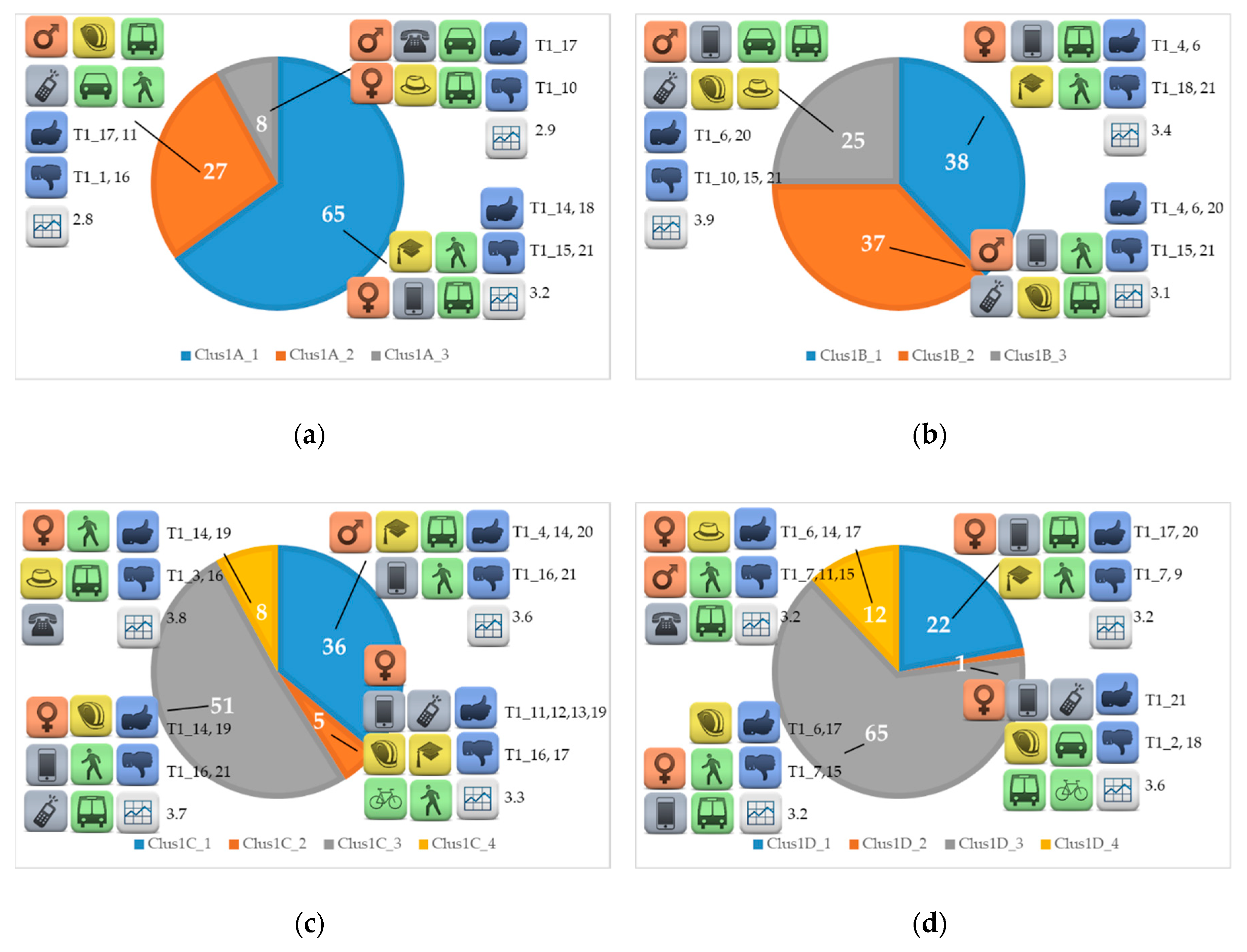
Figure 2.
Graphical representation of the characteristics of the clusters obtained with the approach Clus2 for: (a) city A; (b) city B; (c) city C; (d) city D.
Figure 2.
Graphical representation of the characteristics of the clusters obtained with the approach Clus2 for: (a) city A; (b) city B; (c) city C; (d) city D.

Table 1.
Partitions of the cleaned dataset in the four cities for the features considered in the analysis.
Table 1.
Partitions of the cleaned dataset in the four cities for the features considered in the analysis.
| Category | Collective Variable | Feature | City A | City B | City C | City D |
|---|---|---|---|---|---|---|
| Gender | Male | Male | 54.4% | 51.4% | 41.5% | 39.2% |
| Female | Female | 45.6% | 48.2% | 58.3% | 60.8% | |
| Other | Other | 0.0% | 0.4% | 0.2% | 0.0% | |
| Age | Young | <17 | 0.0% | 2.5% | 8.7% | 0.0% |
| 18–24 | 49.5% | 33.3% | 28.2% | 19.9% | ||
| 25–34 | 8.7% | 21.7% | 21.4% | 37.2% | ||
| Adult | 35–44 | 13.6% | 18.3% | 17.0% | 17.6% | |
| 45–54 | 13.6% | 11.9% | 12.5% | 8.4% | ||
| 55–64 | 5.8% | 6.5% | 4.7% | 6.8% | ||
| Aged | 65–74 | 4.9% | 4.9% | 6.2% | 9.1% | |
| 75+ | 3.9% | 0.9% | 1.3% | 1.0% | ||
| Working status | Worker | Full time | 14.6% | 44.3% | 33.8% | 55.1% |
| Part-time | 2.9% | 7.0% | 11.1% | 7.1% | ||
| Self-employed | 16.5% | 4.0% | 3.3% | 3.7% | ||
| Student | Student | 45.6% | 21.7% | 32.0% | 13.9% | |
| Working student | 2.9% | 9.6% | 9.8% | 4.4% | ||
| Not working | Unemployed | 1.9% | 3.4% | 3.1% | 3.0% | |
| Pensioner | 8.8% | 4.9% | 6.1% | 11.1% | ||
| Housewife/husband | 6.8% | 1.1% | 0.8% | 0.3% | ||
| Other | Other | 0.0% | 4.0% | 0.0% | 1.4% |
Table 2.
Distribution of modes use and modes combinations in the four cities.
| Number of Modes | Mode Combinations | City A | City B | City C | City D |
|---|---|---|---|---|---|
| 1 | IM | 6.8% | 1.8% | 8.5% | 6.8% |
| BI | 0.0% | 0.2% | 2.7% | 0.3% | |
| PT | 3.9% | 28.6% | 39.1% | 26.7% | |
| WA | 1.0% | 0.9% | 1.8% | 1.4% | |
| OT | 1.0% | 0.0% | 0.4% | 2.4% | |
| Total | 12.7% | 31.5% | 52.5% | 37.6% | |
| 2 | IM BI | 1.0% | 0.0% | 0.0% | 0.3% |
| IM PT | 4.8% | 10.1% | 1.3% | 3.1% | |
| IM WA | 6.8% | 0.2% | 0.9% | 0.0% | |
| IM OT | 0.0% | 0.0% | 0.2% | 0.0% | |
| BI PT | 0.0% | 0.7% | 0.2% | 0.0% | |
| BI WA | 0.0% | 0.0% | 0.5% | 0.0% | |
| PT WA | 71.8% | 43.8% | 39.3% | 53.0% | |
| PT OT | 0.0% | 0.7% | 0.2% | 1.7% | |
| WA OT | 0.0% | 0.0% | 0.0% | 0.3% | |
| Total | 84.4% | 55.5% | 42.6% | 58.4% | |
| 3 | IM BI PT | 0.0% | 0.2% | 0.2% | 0.3% |
| IM PT WA | 1.0% | 10.5% | 2.4% | 2.4% | |
| IM PT OT | 0.0% | 0.5% | 0.2% | 0.0% | |
| BI PT WA | 0.0% | 0.7% | 1.6% | 0.0% | |
| PT WA OT | 1.9% | 0.9% | 0.5% | 1.0% | |
| Total | 2.9% | 12.8% | 4.9% | 3.7% | |
| 4 | IM PT WA OT | 0.0% | 0.2% | 0.0% | 0.3% |
| Total | 0.0% | 0.2% | 0.0% | 0.3% |
IM: individual modes, BI: bicycle, PT: public transport, WA: walking, OT: other.
Table 3.
T1 questions and codification of the indicators, with the mean values for each city.
| Question ID | T1 Category Name | City A | City B | City C | City D |
|---|---|---|---|---|---|
| T1_1 | Design of stations was adequate for my needs | 2.6 | 3.5 | 3.7 | 3.3 |
| T1_2 | Design of transport interchanges (main terminals) was efficient | 2.7 | 3.4 | 3.6 | 3.2 |
| T1_3 | Design of transport stops was adequate for my needs | 2.8 | 3.4 | 3.7 | 3.2 |
| T1_4 | The city supported my mobility needs | 3.0 | 3.9 | 3.8 | 3.1 |
| T1_5 | The different modes of transport I used worked well together | 2.8 | 3.4 | 3.7 | 3.1 |
| T1_6 | My passenger rights (e.g., able to access all transport services) were respected | 2.7 | 3.9 | 3.8 | 3.5 |
| T1_7 | The overall accessibility of my journey was adequate for travellers with additional needs | 3.2 | 3.5 | 3.4 | 2.8 |
| T1_8 | Provision of information on arrivals and departures was adequate for my needs | 2.8 | 3.3 | 3.8 | 3.0 |
| T1_9 | Public transport staff were receptive to my needs | 3.4 | 3.4 | 3.4 | 2.9 |
| T1_10 | The quality of travel information available during journey was good | 2.5 | 3.1 | 3.6 | 3.1 |
| T1_11 | The quality of pre-trip information before I started my journey was good | 3.2 | 3.2 | 3.8 | 3.1 |
| T1_12 | The quality of transport infrastructure (e.g., whole transport service) during my journey was good | 3.2 | 3.2 | 3.8 | 3.1 |
| T1_13 | The quality of my ride was good | 3.5 | 3.4 | 3.8 | 3.3 |
| T1_14 | My safety and security while travelling was good | 3.8 | 3.7 | 3.9 | 3.5 |
| T1_15 | Support for intermodal (e.g., different forms of transport during same journey) travel was provided | 2.3 | 3.1 | 3.6 | 2.9 |
| T1_16 | Recognition of the needs of motorised vehicle users | 3.1 | 3.4 | 3.3 | 3.0 |
| T1_17 | Ticket purchasing process was easy to follow | 3.6 | 3.8 | 3.4 | 3.6 |
| T1_18 | Time the journey took was as promised | 3.7 | 3.2 | 3.7 | 3.4 |
| T1_19 | Transport availability was adequate for my needs | 3.4 | 3.3 | 3.9 | 3.3 |
| T1_20 | Vehicle design was suitable for my needs | 3.5 | 3.8 | 3.8 | 3.5 |
| T1_21 | Value for money of services was good | 2.4 | 3.0 | 3.2 | 3.2 |
| Mean value | 3.1 | 3.4 | 3.6 | 3.2 |
Table 4.
Characteristics of the clusters obtained with approach Clus1.
| Test Site | Cluster | Gender | Age | Working Status | Transport Modes | T1 Indicators | |||||||||||
|---|---|---|---|---|---|---|---|---|---|---|---|---|---|---|---|---|---|
| % | Male | Female | Young | Adult | Aged | Worker | Student | Not Working | IM | BI | PT | WA | Mean | Max | Min | ||
| City A | Clus1A_1 | 65 | x | x | x | x | x | 3.2 | T1_14, 18 | T1_15, 21 | |||||||
| Clus1A_2 | 27 | x | x | x | x | x | x | 2.8 | T1_17, 11 | T1_1, 16 | |||||||
| Clus1A_3 | 8 | x | x | x | x | x | x | 2.9 | T1_17 | T1_10 | |||||||
| City B | Clus1B_1 | 38 | x | x | x | x | x | 3.4 | T1_4, 6 | T1_18, 21 | |||||||
| Clus1B_2 | 37 | x | x | x | x | x | x | 3.1 | T1_4, 6, 20 | T1_15, 21 | |||||||
| Clus1B_3 | 25 | x | x | x | x | x | x | x | 3.9 | T1_6, 20 | T1_10, 15, 21 | ||||||
| City C | Clus1C_1 | 36 | x | x | x | x | x | 3.6 | T1_4, 14, 20 | T1_16, 21 | |||||||
| Clus1C_2 | 5 | x | x | x | x | x | x | x | 3.3 | T1_11, 12, 13, 19 | T1_16, 17 | ||||||
| Clus1C_3 | 51 | x | x | x | x | x | x | 3.7 | T1_14, 19 | T1_16, 21 | |||||||
| Clus1C_4 | 8 | x | x | x | x | x | 3.8 | T1_14, 19 | T1_3, 16 | ||||||||
| City D | Clus1D_1 | 22 | x | x | x | x | x | 3.2 | T1_17, 20 | T1_7, 9 | |||||||
| Clus1D_2 | 1 | x | x | x | x | x | x | x | 3.6 | T1_21 | T1_2, 18 | ||||||
| Clus1D_3 | 65 | x | x | x | x | x | 3.2 | T1_6, 17 | T1_7, 15 | ||||||||
| Clus1D_4 | 12 | x | x | x | x | x | x | 3.2 | T1_6, 14, 17 | T1_7, 11, 15 | |||||||
Table 5.
Characteristics of the clusters obtained with approach Clus2.
| Test Site | Cluster | Gender | Age | Working Status | Transport Modes | T1 Indicators | ||||||||||
|---|---|---|---|---|---|---|---|---|---|---|---|---|---|---|---|---|
| % | Male | Female | Young | Adult | Aged | Worker | Student | Not Working | IM | PT | WA | Mean | Max | Min | ||
| City A | Clus2A_1 | 51 | x | x | x | x | x | 3.2 | T1_14, 18 | T1_15, 21 | ||||||
| Clus2A_2 | 19 | x | x | x | x | x | 2.8 | T1_13, 14 | T1_3, 7, 15, 21 | |||||||
| Clus2A_3 | 20 | x | x | x | x | x | x | 3.1 | T1_11, 17 | T1_9, 10, 16 | ||||||
| Clus2A_4 | 10 | x | x | x | x | x | 2.9 | T1_17 | T1_5, 10 | |||||||
| City B | Clus2B_1 | 25 | x | x | x | x | x | 3.7 | T1_6, 17 | T1_18, 21 | ||||||
| Clus2B_2 | 18 | x | x | x | x | x | x | x | 4.2 | T1_6, 20 | T1_15, 21 | |||||
| Clus2B_3 | 52 | x | x | x | x | x | x | 2.9 | T1_4, 6, | T1_15, 21 | ||||||
| Clus2B_4 | 5 | x | x | x | x | x | 4.6 | T1_6, 9, 13, 14 | T1_7, 10 | |||||||
| City C | Clus2C_1 | 34 | x | x | x | x | x | 3.6 | T1_4, 14 | T1_16, 21 | ||||||
| Clus2C_2 | 14 | x | x | x | x | x | 3.7 | T1_13, 14, | T1_16, 21 | |||||||
| Clus2C_3 | 22 | x | x | x | x | x | x | 4.2 | T1_8, 14 | T1_16, 21 | ||||||
| Clus2C_4 | 24 | x | x | x | x | x | x | 3.1 | T1_14, 18, 19 | T1_7, 21 | ||||||
| Clus2C_5 | 6 | x | x | x | x | x | 4.0 | T1_14, 19 | T1_7, 16 | |||||||
| City D | Clus2D_1 | 17 | x | x | x | x | x | 3.2 | T1_17, 19 | T1_7, 9 | ||||||
| Clus2D_2 | 13 | x | x | x | x | x | 3.5 | T1_13, 14, 20 | T1_7, 15 | |||||||
| Clus2D_3 | 29 | x | x | x | x | x | x | 3.7 | T1_6, 17 | T1_8, 16 | ||||||
| Clus2D_4 | 30 | x | x | x | x | x | 2.5 | T1_17, 20 | T1_7, 8, 9 | |||||||
| Clus2D_5 | 11 | x | x | x | x | x | 3.2 | T1_14, 17 | T1 _11, 15 | |||||||
© 2019 by the authors. Licensee MDPI, Basel, Switzerland. This article is an open access article distributed under the terms and conditions of the Creative Commons Attribution (CC BY) license (http://creativecommons.org/licenses/by/4.0/).
Share and Cite
MDPI and ACS Style
Pirra, M.; Pensa, R.G. Comparing Transport Quality Perception among Different Travellers in European Cities through Co-Cluster Analysis. Sustainability 2019, 11, 7159. https://doi.org/10.3390/su11247159
AMA Style
Pirra M, Pensa RG. Comparing Transport Quality Perception among Different Travellers in European Cities through Co-Cluster Analysis. Sustainability. 2019; 11(24):7159. https://doi.org/10.3390/su11247159
Chicago/Turabian StylePirra, Miriam, and Ruggero G. Pensa. 2019. "Comparing Transport Quality Perception among Different Travellers in European Cities through Co-Cluster Analysis" Sustainability 11, no. 24: 7159. https://doi.org/10.3390/su11247159
Note that from the first issue of 2016, this journal uses article numbers instead of page numbers. See further details here.