Complexity Assessment of Assembly Supply Chains from the Sustainability Viewpoint

Abstract

Assembly supply chain systems are becoming increasingly complex and, as a result, there is more and more need to design and manage them in a way that benefits the producers and also satisfies the interests of community stakeholders. The structural (static) complexity of assembly supply chain networks is one of the most important factors influencing overall system complexity. Structures of such networks can be modeled as a graph, with machines as nodes and material flow between the nodes as links. The purpose of this paper is to analyze existing assembly supply chain complexity assessment methods and propose such complexity metric(s) that will be able to accurately reflect not only specific criteria for static complexity measures, but also selected sustainability aspects. The obtained results of this research showed that selected complexity indicators reflect sustainability facets in different ways, but one of them met the mentioned requirements acceptably.

1. Introduction

In the past decades, product and manufacturing process developments have faced rapidly changing market needs. This global trend has resulted in more complex products and manufacturing processes to produce them. As is well known, assembly processes play a key role in production systems. Therefore, any effort for the improvement and optimization of the assembly process is vital to manufacturing competitiveness, since about 50% of the product cost should be ascribed to the assembly phase [1]. One possible way to improve manufacturing competitiveness is to reduce assembly process complexity and the associated cost. Even though the system complexity is inherent and cannot be avoided, it has to be kept affordable. Before defining system complexity for specific purposes, it is important to present some background on complexity as such. According to Flood and Carson [2], “complexity does not solely exist in things, to be observed from their surface and beneath their surface”. Flood [3] adds that if systems are tangible things, then complexity and system are synonymous, where system is prime. According to Faulconbridge and Ryan [4], “a system necessarily has a boundary through which it or its elements interact with elements or systems outside the boundary”. This system-inherent property allows us to adopt graph complexity measures for the complexity quantification of engineered systems [5]. Reynolds [6] points out that the structural modeling approach is applicable for clearly structured systems, in contrast to the behavioral approach, where structure is not assumed a priori. In the context of the architectural design, system complexity is proportional to the risk that the functional requirements cannot be met [7]. In order to briefly introduce a structural complexity measurement problem, it would be useful to mention the fact that prevalent approaches toward measuring system complexity are based on entropy theory (see, e.g., [8,9,10,11]). Entropy can be interpreted in different ways, but in terms of technical systems, it is construed as a measure of information. This entropy measure was introduced by Shannon and Weaver [12], who reduced the concept of entropy to pure probability theory. Their considerations were adopted by Frizelle and Woodcock [13] in order to define static and dynamic system complexity. In regard to the scope of this paper, our primary concern is static system complexity, defined as the amount of information needed to specify the system and its components. System complexity belongs to general systems theory, because it has been applied to different kinds of systems, including technical, social, and biological networks [14,15,16].

The purpose of this paper is to analyze existing complexity assessment methods to measure assembly supply chain (ASC) complexity and propose accurate complexity metric(s) that will include not only specific criteria for static complexity measures, but also sustainability viewpoints.

2. Related Works

The recent literature offers several different views on the relation between the sustainability and complexity of manufacturing systems, including ASCs. For instance, Peralta et al. [17] argue that it is necessary to establish new approaches that reduce increasing complexity of manufacturing systems in the design and management stage in order to promote their sustainability. For that purpose, they developed a so-called fractal model for sustainable manufacturing. Moldawska [18] proposed a complexity-based model of sustainable manufacturing, assuming that sustainable manufacturing organization tends to maintain its own sustainability, as well as contribute to the sustainability of the world. Relations between supply chains and sustainability were also treated in works [19,20] in which the authors analyzed the effect of distributed manufacturing systems on sustainability. The study [21] explored the influence of mass customization strategy on the configuration complexity of assembly systems, and their authors proposed bounds for configuration complexity scale. ASCs in terms of mass customization can lead to very complex systems due to the high number of product variants. It has been proved that variety itself also has a significant impact on productivity, increased costs, and quality [22,23]. Therefore, such companies need to consider integrating their business practices with sustainability and reducing supply chain costs to achieve a competitive advantage [24,25,26].

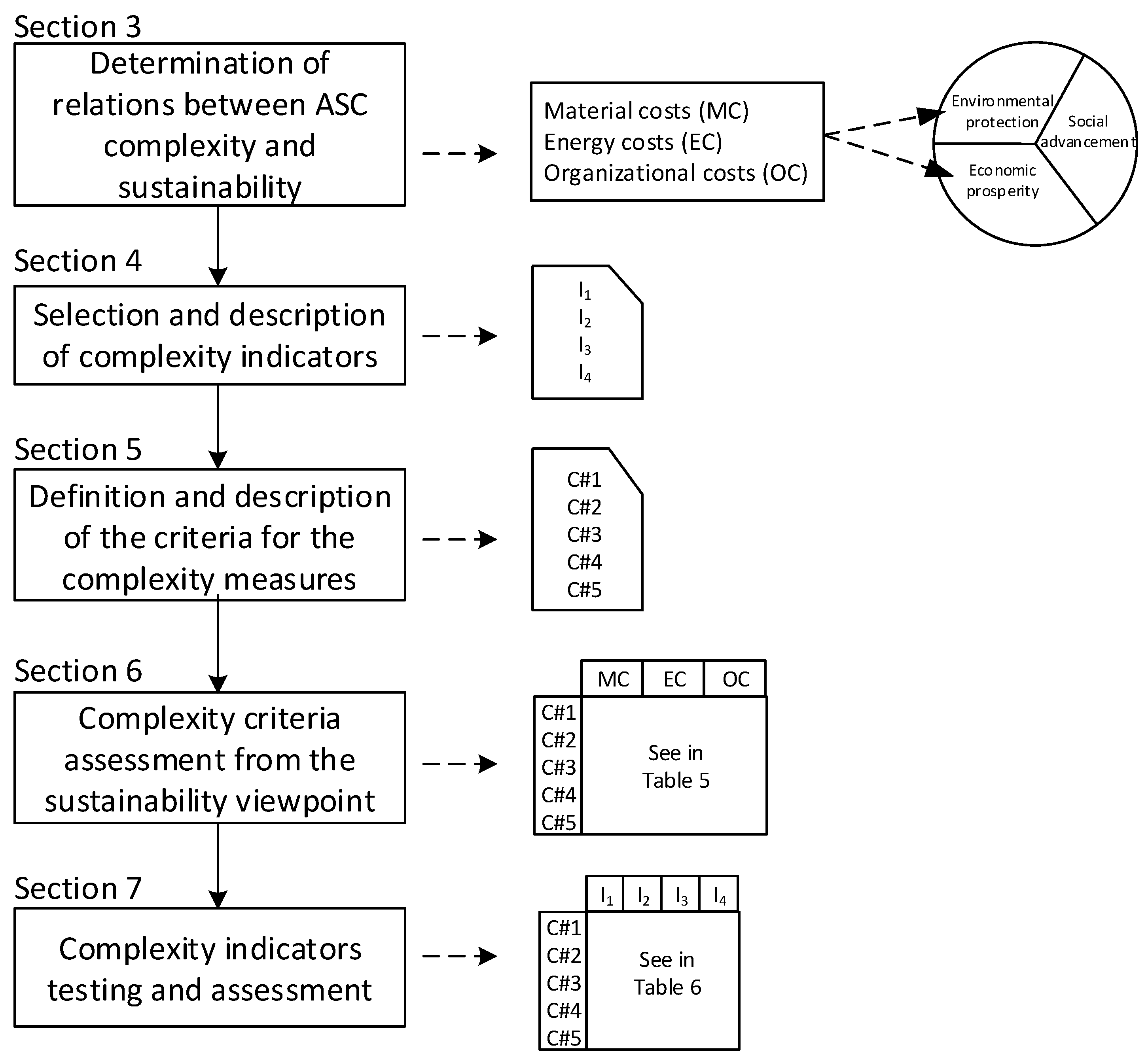
3. Methodology Framework

When exploring the relation between ASC structural complexity and sustainability, one has to consider the fact that lower ASC structural complexity has a positive implication on material costs, energy costs, and organizational costs. Moreover, it is rather clear that the first of the two items are directly related not only to economic burden, but also to environmental quality. Therefore, the two fundamental elements of sustainability practice, i.e., economic prosperity and environmental protection, is further the main subject of our interest in the context of ASCs. Because it is rather complicated to sufficiently estimate the relation between the structural complexity of ASCs and social implications, the social aspect of sustainability in our approach is omitted. Nevertheless, it has to be mentioned that increasing organizational complexity can cause positive implications on social advancement [27]. When comparing the three cost items (material, energy, and organizational), the first two of them can be empirically considered to be more important from a sustainability viewpoint than organizational costs. However, organizational costs have to be perceived as relevant in a given nexus of sustainability practice, since any organizational activity uses materials and energy.

With the aim to fulfill the goal of this research defined in the introduction section with the encompassing above outlined relation between ASC complexity and sustainability, the following methodological framework is proposed and used (see Figure 1).

4. Description of Possible ASC Structural Complexity Indicators

In order to identify reliable and consistent complexity indicator(s), four relevant complexity methods were described and mutually compared, namely index of vertex degree, modified flow complexity, system design complexity, and process complexity indicator.

4.1. Index of Vertex Degree

This indicator was originally developed by Bonchev [28] to quantify the structural complexity of general networks. He adopted Shannon’s information theory by applying the entropy of information H (α) in describing a message of N symbols. Further it is assumed that such symbols are distributed according to some equivalence criterion α into k groups of N₁, N₂, …, N_k symbols. Then, entropy of information H (α) is calculated by the formula:

$$H\left(\alpha \right)=-{{\displaystyle \sum }}_{i=1}^k{p}_{i}lo{g}_2{p}_i=-{{\displaystyle \sum }}_{i=1}^k\frac{N_i}{N}lo{g}_2\frac{N_i}{N},$$

(1)

where p_i specifies the probability of the occurrence of the elements of the ith group.

Further, he substituted symbols or system elements for the vertices, and defined the probability for a randomly chosen system element i to have the weight w_i as p_i = w_i/∑w_i with ∑w_i = w, and ∑p_i = 1.

Then, the probability for a randomly chosen vertex i in the complete graph of V vertices to have a certain degree deg (v)_i can be expressed by the formula:

$$p_i=\frac{\mathrm{deg}{\left(v\right)}_i}{{{\displaystyle \sum }}_{i=1}^V\mathrm{deg}{\left(v\right)}_i}$$

(2)

Assuming that the information can be defined, according Shannon [29], as I = H_max − H, where H_max is the maximum entropy that can exist in a system with the same number of elements, the information entropy of a graph with a total weight W and vertex weights w_i can be expressed in the form of the equation:

$$H\left(W\right)=Wlo{g}_{2}W-{\displaystyle \sum }_{i=1}^V{w}_{i}lo{g}_2{w}_i$$

(3)

Since the maximum entropy is when all w_i = 1, then H_max = Wlog₂W, and by substituting W = ∑deg(v)_i and w_i = deg(v)_i, the information content of the vertex degree distribution of a network, called the vertex degree index (I_vd), is expressed as follows [28]:

$$I_{vd}={\displaystyle \sum }_{i=1}^V\mathrm{deg}{\left(v\right)}_{i}lo{g}_2\mathrm{deg}{\left(v\right)}_i$$

(4)

The vertex degree index was subsequently applied to measure the structural complexity of assembly supply chains, and compared with other existing complexity measures [30].

The selected complexity indicator was applied on the following examples of ASCs by Hamta et al. [31] (see Figure 2). All the five ASCs had the same number of input components, but they differed in the number of operations and the number of machines.

The complexity values obtained by using Equation (4) are shown in

Table 1. Obtained complexity values by I_vd.

Graph	(a)	(b)	(c)	(d)	(e)
Ivd	8 bits	10 bits	9.51 bits	11.51 bits	11.51 bits

.

4.2. Process Complexity Indcator

An additional ASC structural complexity measure that was considered was the so-called process complexity indicator (PCI), which was introduced for the purpose of enumerating the operational complexity of manufacturing processes. Its expression is as follows [32]:

$$PCI=-{\displaystyle \sum _{i=1}^M{\displaystyle \sum _{j=1}^P{\displaystyle \sum _{k=1}^O{p}_{ijk}\cdot {\log }_2{p}_{ijk}}}},$$

(5)

where p_ijk means the probability that part j is being proceeded by operation k by individual machine i based on the scheduling order; O is the number of operations according to parts production; P is the number of parts produced in the manufacturing process; and M is the number of all machines of all types in the manufacturing process.

It is assumed that machines in a given manufacturing process are organized in a serial and/or parallel manner in Equation (5). The probability that part j is being processed due to operation k on an individual machine i is calculated in the following way. In the case when a part is processed on machines in a serial manner, then p_ijk equals 1/M_s, where M_s presents the number of machines organized in serial. In the case when a part is processed on machines in a parallel manner, then p_ijk = 1/M_p, where M_p represents the number of machines organized in parallel. In the case where we have a serial/parallel arrangement of machines and a part is processed on one of the parallel machines, then p_ijk equals 1/M_s.M_p.

The complexity values obtained by using Equation (5) are shown in

Table 2. Obtained complexity values by process complexity indicator (PCI).

Graph	(a)	(b)	(c)	(d)	(e)
PCI	0 bits	3 bits	2 bits	4 bits	4.17 bits

.

4.3. System Design Complexity

Guenov [33] proposed three indicators for architectural design complexity measurement based on Boltzmann’s entropy theory (see, e.g., [34]) and axiomatic design theory [35]. Those indicators can be principally applied also as ASC complexity measures. However, only one of them has been treated as a potential indicator to measure ASC structural complexity [36]. Its description is as follows. Let us denote N as the number of interactions within a design matrix, and N₁, N₂, …, N_k as the numbers of interactions per each design parameter (DP) of the same matrix. Then, the so-called degree of disorder W can be expressed by the formula:

$$\mathsf{\Omega }=C_N^{N_1}*C_{N-N_1}^{N_2}*C_{N-N_1-N_2}^{N_3}\dots *\dots C_{N-N_1-\dots -N_{K-1}}^{N_K}=\frac{N!}{N_1!N_2!\dots N_K!},$$

(6)

where:

$$C_N^{N_1}=\frac{N!}{\left(N-N_1\right)!N_1!}$$

(7)

The multiplicity Ω in Equation (6) is often called the degree of disorder.

The state of gas body g at a given time t where the gas body consists of N molecules, each characterized by n magnitudes φ_j was considered by Boltzmann. For each magnitude φ_j, its interval of admitted values is divided into small intervals of equal length ∆_j. Then, the n-dimensional space, also known as µ-space or module space, can be divided into a system of cells of equal volume: υ^µ = ∆_i,…, ∆_n. K is the number of these cells in the total range of admitted values, R^µ; then: υ^µ = V^µ/K, where V^µ is the volume of R^µ. The µ-cells are analogous to the cells Q_j (j = 1, …, K) in the classification system. f_j means the density in Q_j, i.e., the number of molecules per unit of µ-volume: f_j = N_j/υ^µ. The function defined by Boltzmann for a statistical description is:

$$\mathrm{H}={\displaystyle \sum }_{j=1}^K\left[f_{j}ln{f}_j\right]{\upsilon }^{\mu }$$

(8)

According to Equation (8) and f_j = N_j/υ^µ, where the volume is assumed equal to unity, the following formula for complexity measure can be derived:

$$\sum N_{j}ln{N}_j$$

(9)

where N_j is interpreted as the number of interactions per single DP.

Its application to measure the structural complexity of ASC was provided by Modrak and Soltysova [37], where the model of assembly process is structured with two groups of objects, while the first group is denoted as input components (ICs) and the second group as workstations. The input components are assembled at these workstations. Then, for the purpose of measuring process complexity, the following transformation is proposed: ICs are substituted by DPs, according to relation DPs = B. PVs (where PVs mean process variables and B is the design matrix that defines the characteristics of the process design) and workstations are considered as PVs. Subsequently, the assembly process structure is transformed into design matrix (DM) with DP–PV relations and finally, the structural complexity of ASC can be enumerated.

The complexity values obtained by using Equation (9) are shown in

Table 3. Obtained complexity values by system design complexity (SDC).

Graph	(a)	(b)	(c)	(d)	(e)
SDC	5.55 nats	8.84 nats	6.93 nats	8.32 nats	10.23 nats

.

4.4. Modified Flow Complexity

The next possible ASC complexity indicators were developed by Crippa [38]. The most suitable indicator of these is considered to be the so-called modified flow complexity (MFC) indicator. The MFC indicator enumerates all tiers (including Tier 0), nodes, and links and adds all these counts, weighted with determined α, β, and γ and coefficients. Nodes and links are counted only once, even if they are repeated in the graph. Node and link repetition is included in coefficients. The MFC indicator can be enumerated by the following equations [38]:

$$MFC=\alpha .T+ \beta .N+\gamma .L$$

(10)

$$\alpha =MTI=\frac{TN-N}{\left(T-1\right).N}$$

(11)

$$\beta =MTR=\frac{TN}{N}$$

(12)

$$\gamma =MLR=\frac{LK}{L}$$

(13)

where MTI is multi-tier index; MTR is multi-tier ratio; MLR is multi-link ratio; N is the number of nodes; TN is the number of nodes per ith tier level; L is number of links; LK is number of links per ith tier level; T is the number of tiers.

The complexity values obtained by using Equation (10) are shown in

Table 4. Obtained values enumerated by modified flow complexity (MFC).

Graph	(a)	(b)	(c)	(d)	(e)
MFC	9	11	11	13	13

.

5. Definition of Testing Rules for ASC Complexity Indicators

To prove the selected complexity indicators, all of them were verified through defined criteria for complexity measures that might also be taken into account to assess their validity. Such rules were specified and proposed for static complexity metrics by Deshmuk et al. [9] and Olbrich et al. [39]. Deshmuk et al. [9] analyzed different factors influencing the static complexity of manufacturing systems, and defined four conditions that the static complexity metric must satisfy. They are as follows [9]:

Rule#1:

Static complexity should increase with the number of parts and the number of machines and operations required to process the part mix.

Rule#2:

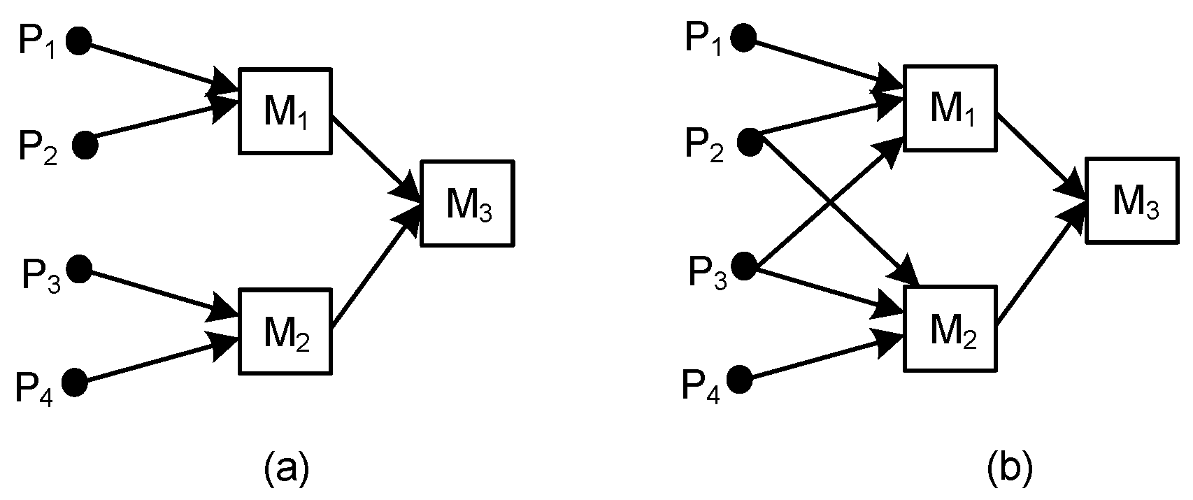
Static complexity should increase with increases in sequence flexibility for the parts in the production batch.

Rule#3:

Static complexity should increase as the sharing of resources by parts increases.

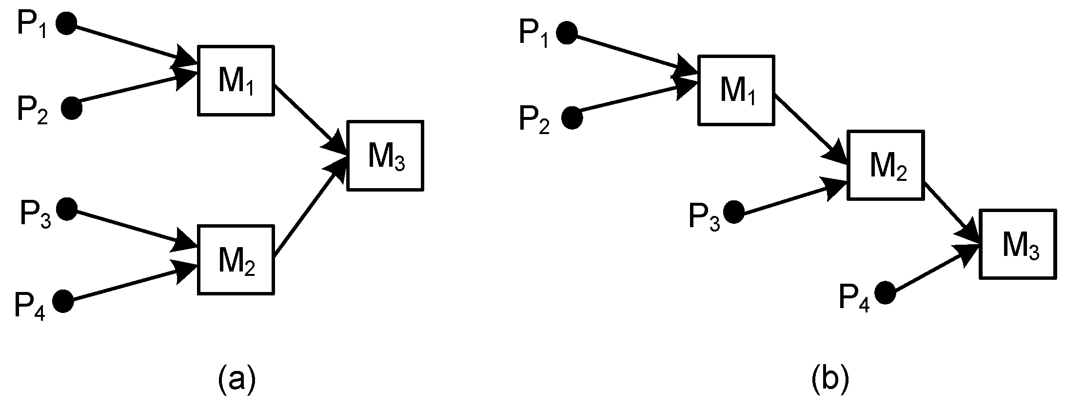
Rule#4:

If the original part mix is split into two or more groups, then the complexity of processing should remain constant.

Due to the fact that Rule#3 and Rule#4 are not relevant for assembly supply chains, only two of them were adopted in terms of ASC systems.

Olbrich et al. [39] studied how static complexity measures behave if the system size is increased and explored three special cases of adding an independent element, two independent subsystems, and two identical copies. In this context, the authors proposed three specific requirements or rules for a reliable complexity measure that must be met:

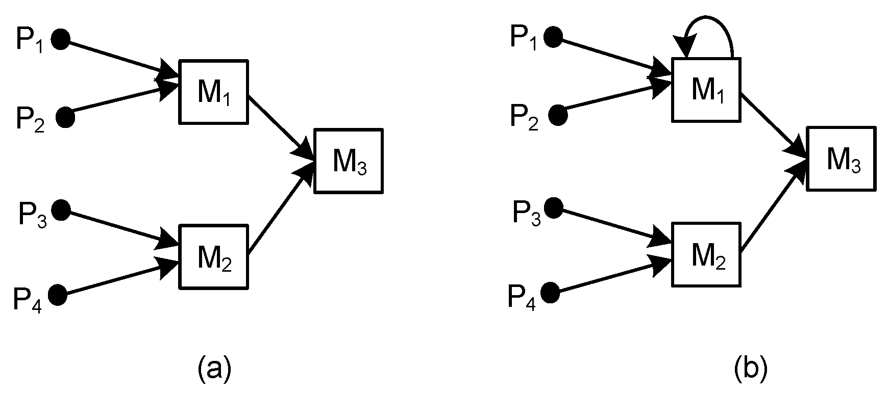
Rule#1:

Additional independent element: The element has no structure itself, so it has no complexity of its own. Because it is independent of the rest of the system, the complexity should not change.

Rule#2:

Union of two independent systems: Because there are no dependencies between the two systems, the complexity of the union should be simply the sum of the complexities of the subsystems.

Rule#3:

Union of two identical copies: Because there is no need for additional information to describe the second system, one could argue that the complexity should be equal to the complexity of one system. One has, however, to include the fact in the description that the second system is a copy of the first one. At least this part should not be extensive with respect to the system size.

However, any of the three rules appear to be impactful for ASC complexity metrics, and therefore were not directly used for the purpose of testing and comparing the complexity indicators.

After deeper consideration, the two rules by Deshmuk et al. [9], namely Rules 1 and 2, were adopted by us into the four testing criteria (C). Moreover, we added one additional criterion (C#5) based on the increasing number of echelons. The criteria are summarily shown as follows:

C#1: 

Static complexity should increase with the number of parts required to process the part mix.

C#2: 

Static complexity should increase with the number of machines required to process the part mix.

C#3: 

Static complexity should increase with the number of operations required to process the part mix.

C#4: 

Static complexity should increase with increases in sequence flexibility for the parts in the production batch.

C#5: 

Static complexity should increase with the number of echelons while the number of parts, machines, and operations is constant.

6. Analysis of Testing Criteria from Sustainability Viewpoint

Our description of relations between ASC structural complexity and sustainability seems to be useful to categorize the abovementioned testing criteria based on their importance to the sustainability objectives. In any given case, it was expected that the complexity indicators would reflect the three sustainability facets, i.e.:

• (Direct) energy costs;
• (Direct) material costs;
• (Direct) organizational costs.

Therefore, each of the criteria might validate at least one of the three cost items. By analyzing how these criteria reflect the abovementioned cost items, it can be found that they cover a different number of the cost items. Summarily, these differences are shown in

Table 5. Testing criteria and their reflection on cost items.

Testing Criteria	Material Costs	Energy Costs	Organizational Costs
C#2	✔	✔	✔
C#3	-	✔	✔
C#1	-	-	✔
C#4	-	-	✔
C#5	-	-	✔

.

As can be seen, all criteria include in themselves organizational costs. C#3 moreover covers energy costs and C#2 relates to all of the cost items. This viewpoint was further applied for the purpose of comparing the usability of ASC complexity indicators.

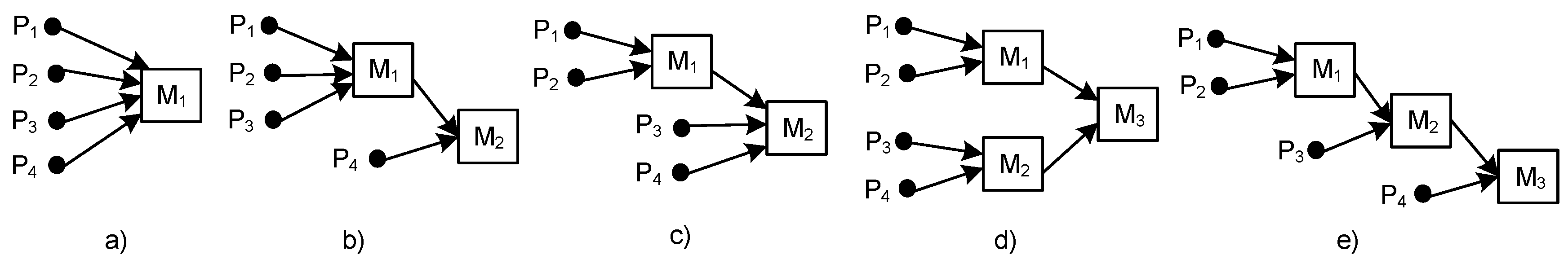
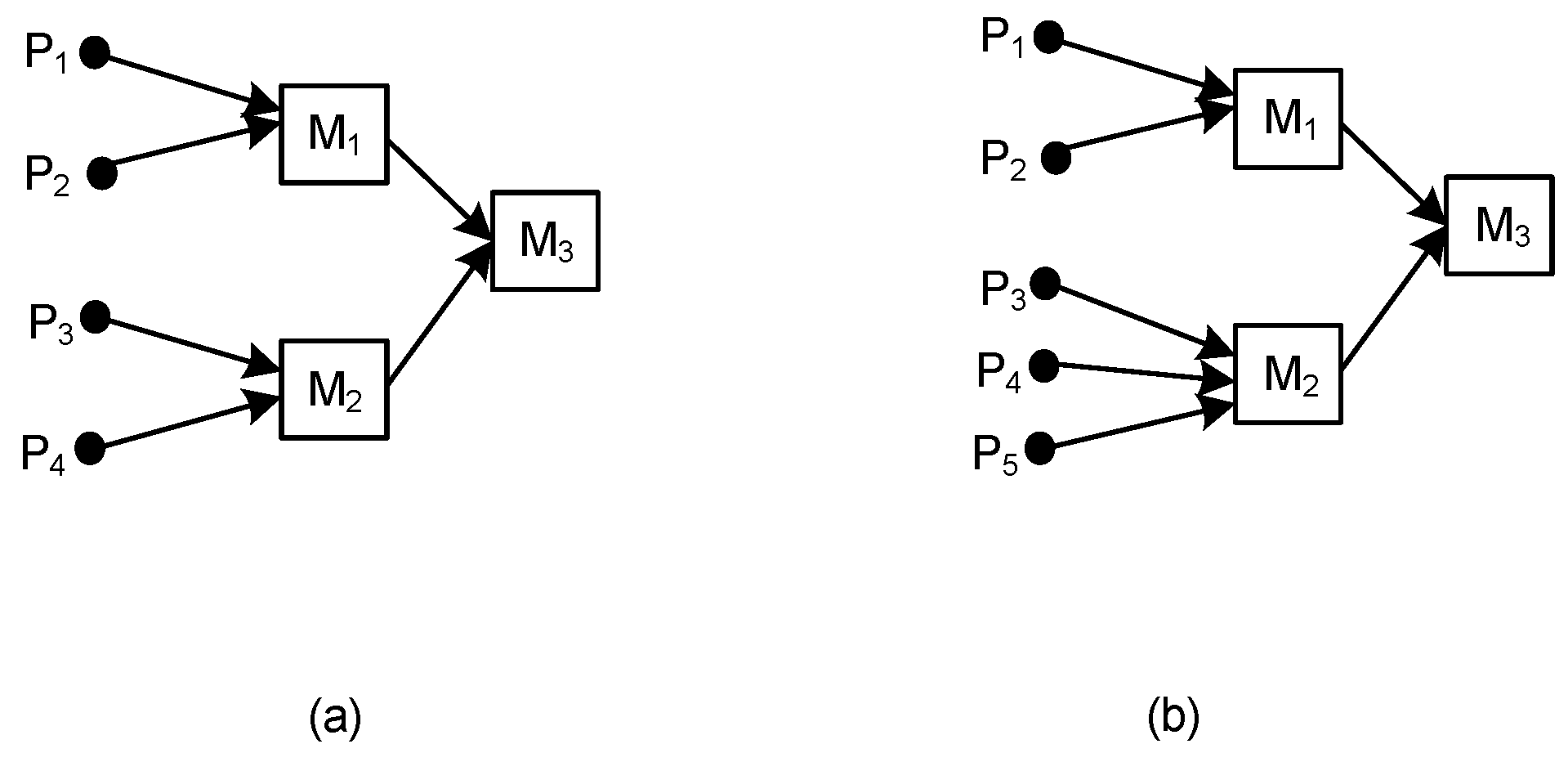
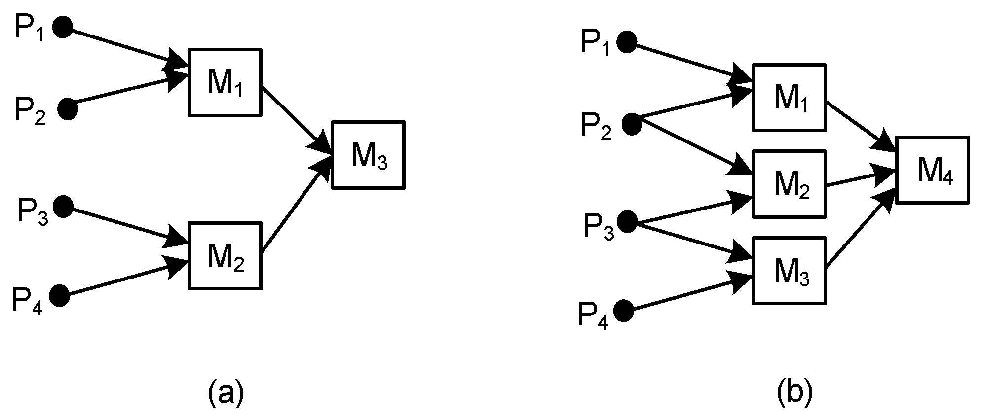
7. Testing and Comparison of ASC Complexity Indicators

This part of the paper is focused on the comparison of two assembly supply chains, ASC₁(i,j,k) and ASC₂(i,j,k). One of them is more complex according to the defined criteria (C#1–C#5). P represents parts, j is the number of parts, O represents operations, k is the number of operations, M represents machines, and i is the number of machines.

These criteria were tested using the theoretical examples shown in Figure 3, Figure 4, Figure 5, Figure 6 and Figure 7. In C#1, #2, #4, and #5, the number of machines was equal to the number of operations. In C#3, the number of operations was increasing.

7.1. Testing of C#1

C#1 is proposing the following statement:

If i is constant (i = k) and j is increasing, then the structural complexity of ASC(i,j-1,k) < ASC(i,j,k).

Let us test ASC₁(3;4;3) and ASC₂(3;5;3), shown in Figure 3. While in Figure 3a, ASC₁ consists of three machines and operations (i = k = 3), and the number of parts equals four (j = 4), in Figure 3b, ASC₂ contains three machines and operations (i = k = 3), and the number of parts equals five (j = 5).

Applying Equation (4), according to complexity indicator I_vd, we obtained the following results for static complexity using I_vd1 (for ASC₁) and I_vd2 (for ASC₂):

I_vd1 = 3 × log₂3 + 3 × log₂3 + 2 × log₂2 = 11.51 bits

I_vd2 = 3 × log₂3 + 4 × log₂4 + 2 × log₂2 = 14.76 bits

Applying Equation (5), according to complexity indicator PCI, we obtained the following results for PCI₁ and PCI₂:

PCI₁ = −(0.5 × log₂0.5 + 0.5 × log₂0.5 + 0.5 × log₂0.5 + 0.5 × log₂0.5) = 4 bits

PCI₂ = −(0.5 × log₂0.5 + 0.5 × log₂0.5 + 0.5 × log₂0.5 + 0.5 × log₂0.5 + 0.5 × log₂0.5 + 0.5 × log₂0.5) = 5 bits

Applying Equation (9), according to complexity indicator system design complexity (SDC), we obtained the following results for SDC₁ and SDC₂:

SDC₁ = 4 × ln4 + 2 × ln2 + 2 × ln2 = 8.32 nats

SDC₂ = 5 × ln5 + 2 × ln2 + 3 × ln3 = 12.73 nats

Applying Equation (10), according to complexity indicator MFC, we obtained the following results for MFC₁ and MFC₂:

MFC₁ = 0 × 3 + 1 × 7 + 1 × 6 = 13

MFC₂ = 0 × 3 + 1 × 8 + 1 × 7 = 15

According to these complexity indicators, it was proved that the complexity of ASC₁(3,4,3) < ASC₂(3,5,3), then ASC(i,j−1,k) < ASC(i,j,k).

7.2. Testing of C#2

C#2 is proposing the following statement:

If j is constant and i is increasing (i = k), then the structural complexity of ASC(i−1,j,k) ˂ ASC(i,j,k).

Let us test ASC₁(3,4,3) and ASC₂(4,4,4), shown in Figure 4. While in Figure 4a, ASC₁ consists of three machines and operations (i = k = 3), and the number of parts equals four (j = 4), in Figure 4b, ASC₂ contains four machines and operations (i = k = 4), and the number of parts equals four (j = 4).

Applying Equation (4), according to complexity indicator I_vd, we obtained the following results for I_vd1 and I_vd2:

I_vd1 = 3 × log₂3 + 3 × log₂3 + 2 × log₂2 = 11.51 bits

I_vd2 = 3 × log₂3 + 3 × log₂3 + 3 × log₂3 + 3 × log₂3 = 19.02 bits

Applying Equation (5), according to complexity indicator PCI, we obtained the following results for PCI₁ and PCI₂:

PCI₁ = −(0.5 × log₂0.5 + 0.5 × log₂0.5 + 0.5 × log₂0.5 + 0.5 × log₂0.5) = 4 bits

PCI₂ = −(0.5 × log₂0.5 + 0.5 × log₂0.5 + 0.25 × log₂0.25 + 0.25 × log₂0.25 + 0.5 × log₂0.5 + 0.25 × log₂0.25 + 0.25 × log₂0.25 + 0.5 × log₂0.5 + 0.5 × log₂0.5 + 0.5 × log₂0.5) = 5 bits

Applying Equation (9), according to complexity indicator SDC, we obtained the following results for SDC₁ and SDC₂:

SDC₁ = 4 × ln4 + 2 × ln2 + 2 × ln2 = 8.32 nats

SDC2 = 4 × ln4 + 2 × ln2 + 2 × ln2 + 2 × ln2 = 9.7 nats

Applying Equation (10), according to complexity indicator MFC, we obtained the following results for MFC₁ and MFC₂:

MFC₁ = 0 × 3 + 1 × 7 + 1 × 6 = 13

MFC₂ = 0 × 3 + 1 × 8 + 1 × 9 = 17

According to these complexity indicators, it was proved that ASC₁(3,4,3) < ASC₂(4,4,4), then ASC(i−1,j,k) ˂ ASC(i,j,k).

7.3. Testing of C#3

C#3 is proposing the following statement:

If i and j are constant and k is increasing, then the structural complexity of ASC(i,j,k−1) ˂ ASC(i,j,k).

Let us test ASC₁(3,4,3) and ASC₂(3,4,4), shown in Figure 5. While in Figure 5a, ASC₁ consists of three machines and operations (i = k = 3), and the number of parts equals four (j = 4), in Figure 5b, ASC₂ contains three machines (i = 3), four operations (k = 4), and the number of parts equals four (j = 4).

Applying Equation (4), according to complexity indicator I_vd, we obtained the following results for I_vd1 and I_vd2:

I_vd1 = 3 × log₂3 + 3 × log₂3 + 2 × log₂2 = 11.51 bits

I_vd2 = 5 × log₂5 + 3 × log₂3 + 2 × log₂2 = 18.37 bits

Applying Equation (5), according to complexity indicator PCI, we obtained the following results for PCI₁ and PCI₂:

PCI₁ = −(0.5 × log₂0.5 + 0.5 × log₂0.5 + 0.5 × log₂0.5 + 0.5 × log₂0.5) = 4 bits

PCI₂ = −(0.25 × log₂0.25 + 0.25 × log₂0.25 + 0.5 × log₂0.5 + 0.25 × log₂0.25 + 0.25 × log₂0.25 + 0.5 × log₂0.5 + 0.5 × log₂0.5 + 0.5 × log₂0.5 + 0.5 × log₂0.5 + 0.5 × log₂0.5) = 5 bits

Applying Equation (9), according to complexity indicator SDC, we obtained the following results for SDC₁ and SDC₂:

SDC₁ = 4 × ln4 + 2 × ln2 + 2 × ln2 = 8.32 nats

SDC₂ = 4 × ln4 + 2 × ln2 + 2 × ln2 = 8.32 nats

Applying Equation (10), according to complexity indicator MFC, we obtained the following results for MFC₁ and MFC₂:

MFC₁ = 0 × 3 + 1 × 7 + 1 × 6 = 13

MFC₂ = 0 × 3 + 1 × 7 + 1 × 7 = 14

According to the three complexity indicators I_vd, PCI, and MFC, it was proved that the structural complexity of ASC₁(3,4,3) < ASC₂(3,4,4), then ASC(i,j,k−1) ˂ ASC(i,j,k).

7.4. Testing of C#4

C#4 is proposing the following statement:

If i, j, and k are constant and the number of routings is increasing, then the structural complexity of ASC(i,j,k) ˂ ASC(i,j,k) with an increasing number of routings.

Let us test ASC₁(3,4,3) and ASC₂(3,4,3), shown in Figure 6. While in Figure 6a, ASC₁ consists of three machines and operations (i = k = 3), and the number of parts equals four (j = 4), in Figure 6b, ASC₂ consists of three machines and operations (i = k = 3), and the number of parts equals four (j = 4), but P₂ and P₃ can be processed on M₁ or M₂.

Applying Equation (4), according to complexity indicator I_vd, we obtained the following results for I_vd1 and I_vd2:

I_vd1 = 3 × log₂3 + 3 × log₂3 + 2 × log₂2 = 11.51 bits

I_vd2 = 4 × log₂4 + 4 × log₂4 + 2 × log₂2 = 18 bits

Applying Equation (5), according to complexity indicator PCI, we obtained the following results for PCI₁ and PCI₂:

PCI₁ = −(0.5 × log₂0.5 + 0.5 × log₂0.5 + 0.5 × log₂0.5 + 0.5 × log₂0.5) = 4 bits

PCI₂ = −(0.5 × log₂0.5 + 0.5 × log₂0.5 + 0.25 × log₂0.25 + 0.25 × log₂0.25 + 0.5 × log₂0.5 + 0.25 × log₂0.25 + 0.25 × log₂0.25 + 0.5 × log₂0.5 + 0.5 × log₂0.5 + 0.5 × log₂0.5) = 5 bits

Applying Equation (9), according to complexity indicator SDC, we obtained the following results for SDC₁ and SDC₂:

SDC₁ = 4 × ln4 + 2 × ln2 + 2 × ln2 = 8.32 nats

SDC₂ = 4 × ln4 + 3 × ln3 + 3 × ln3 = 12.14 nats

Applying Equation (10), according to complexity indicator MFC, we obtained the following results for MFC₁ and MFC₂:

MFC₁ = 0 × 3 + 1 × 7 + 1 × 6 = 13

MFC₂ = 0 × 3 + 1 × 7 + 1 × 8 = 15

According to these complexity indicators, it was proved that the complexity of ASC₁ ˂ ASC₂, then ASC(i,j,k) ˂ ASC(i,j,k) with an increasing number of routings.

7.5. Testing of C#5

C#5 is proposing the following statement:

If i, j, and k are constant and the number of echelons is increasing, then the complexity of ASC(i,j,k) ˂ ASC(i,j,k) with an increasing number of echelons.

Let us test ASC₁(3,4,3) and ASC₂(3,4,3), shown in Figure 7. While in Figure 7a, ASC₁ consists of three machines and operations (i = k = 3), the number of parts equals four (j = 4), and the number of echelons equals two, in Figure 7b, ASC₂ contains three machines (i = 3), four operations (k = 4), the number of parts equals four (j = 4), and the number of echelons equals three.

Applying Equation (4), according to complexity indicator I_vd, we obtained the following results for I_vd1 and I_vd2:

I_vd1 = 3 × log₂3 + 3 × log₂3 + 2 × log₂2 = 11.51 bits

I_vd2 = 3 × log₂3 + 3 × log₂3 + 2 × log₂2 = 11.51 bits

Applying Equation (5), according to complexity indicator PCI, we obtained the following results for PCI₁ and PCI₂:

PCI₁ = −(0.5 × log₂0.5 + 0.5 × log₂0.5 + 0.5 × log₂0.5 + 0.5 × log₂0.5) = 4 bits

PCI₂ = −(0.33 × log₂0.33 + 0.33 × log₂0.33 + 0.33 × log₂0.33 + 0.33 × log₂0.33 + 0.33 × log₂0.33 + 0.33 × log₂0.33 + 0.5 × log₂0.5 + 0.5 × log₂0.5 + 1 × log₂1) = 4.17 bits

Applying Equation (9), according to complexity indicator SDC, we obtained the following results for SDC₁ and SDC₂:

SDC₁ = 4 × ln4 + 2 × ln2 + 2 × ln2 = 8.32 nats

SDC₂ = 4 × ln4 + 3 × ln3 + 2 × ln2 = 10.23 nats

Applying Equation (10), according to complexity indicator MFC, we obtained the following results for MFC₁ and MFC₂:

MFC₁ = 0 × 3 + 1 × 7 + 1 × 6 = 13

MFC₂ = 0 × 4 + 1 × 7 + 1 × 6 = 13

According to the three complexity indicators PCI, SDC, and MFC, it was proved that the complexity of ASC₁ ˂ the complexity of ASC₂, then ASC(i,j,k) ˂ ASC(i,j,k) with an increasing number of echelons.

7.6. Comparison and Selection of ASC Complexity Measure

A mutual comparison of ASC complexity methods is shown in the following

Table 6. Mutual comparison of ASC complexity methods.

Criteria	Ivd	SDC	MFC	PCI
C#2	✔	✔	✔	✔
C#3	✔	X	✔	✔
C#1	✔	✔	✔	✔
C#4	✔	✔	✔	✔
C#5	X	✔	X	✔

:

Based on the obtained results, it can be seen that PCI for ASCs could be considered as the most suitable.

8. Discussion of Results, Implications and Limitations

Summarizing the obtained results from the testing of the ASC complexity indicators, the following statements can be provided:

(i)

All described indicators sufficiently reflect organizational aspects of ASCs.

(ii)

Three of the complexity indicators, namely, I_vd, MFC, and PCI, can be effectively used to measure ASC complexity in order to identify how ASC structural variants are influencing organizational costs, as well as energy costs.

(iii)

The PCI complexity measure reflects all of the three cost items and covers the two crucial dimensions of sustainability, economic and environmental.

In addition, it has to be emphasized that the impact of ASC complexity on social development can only be anticipated based on the theoretical assumption that higher organizational complexity, induced by a company’s favorable development, could positively influence social sustainability. In such a case, it would be expected that organizational complexity is growing not only along various dimensions, such as production volume, but also with the increasing number of employees [40,41]. However, the related literature is more or less ambivalent about whether organizational complexity has positive or negative effects on firm performance [42]. Moreover, if we consider that organizational complexity is frequently defined as “the amount of differentiation that exists within different elements constituting the organization” [43], then it is rather clear that any of the structural complexity indicators can identify organizational complexity changes within a company. Thus, it cannot be excluded that changes of the internal structural complexity will not impact the organizational complexity. Based on the above formulations, it can be concluded that, when comparing two or several ASC alternative solutions, the one with the lowest structural complexity can be considered as the most sustainable and cost-effective approach. Therefore, structural complexity measures can be primarily used as potential indicators for the indirect assessment of material costs and related energy consumption. This drawback of the presented approach can be seen as the main limitation of the analyzed indicators to reflect ASC complexity along with the sustainability issues.

This evaluation method can be effectively used, especially in terms of small and medium size enterprises (SMEs), since it has been found that SMEs are particularly sensitive to the internal complexity environment, as well as to the external complexity environment [44]. For this reason, SMEs need to pay attention also to the complexity management approach in order to entirely manage their sustainability in a turbulent business environment.

9. Conclusions

Finally, it is useful to emphasize that the presented research construct and obtained findings are pertinent for ASCs for the completion of standard products, i.e., not for those that are mass customized. Mass customization, as a new paradigm, also brings significant changes into the assembly process principles. For example, ASCs in terms of mass customization have to be as modular as possible, and it means that modularity has to be considered as a primary property of ASCs. Taking this fact into consideration, the structural complexity of ASCs can be seen as only a complementary indicator to optimize ASCs. Accordingly, the featured related research could be oriented specially to study relations between the complexity and modularity of ASCs in terms of mass customization.

References

- Fan, J.; Dong, J. Intelligent virtual assembly planning with integrated assembly model. In Proceedings of the IEEE International Conference on Systems, Man and Cybernetics. Conference Theme-System Security and Assurance, Washington, DC, USA, 8 October 2003; pp. 4803–4808. [Google Scholar]
- Flood, R.L.; Carson, E.R. Dealing with Complexity: An Introduction to the Theory and Application of Systems Science, 2nd ed.; Springer Science & Business Media: New York, NY, USA, 2013; pp. 1–280. [Google Scholar]
- Flood, R.L. Liberating systems theory. In Liberating Systems Theory; Springer: Boston, MA, USA, 1990; pp. 11–32. [Google Scholar]
- Faulconbridge, R.I.; Ryan, M.J. Systems Engineering Practice; Argos Press: Canberra, Australian, 2018; pp. 1–320. [Google Scholar]
- Efatmaneshnik, M.; Ryan, M.J. Fundamentals of system complexity measures for systems design. In INCOSE International Symposium; Wiley: Hoboken, NJ, USA, 2015; Volume 25, pp. 876–890. [Google Scholar]
- Reynolds, P.A. Introduction to International Relations, 3rd ed.; Routledge: New York, NY, USA, 2016; pp. 1–358. [Google Scholar]
- Suh, N.P. The Principles of Design; Oxford University Press: New York, NY, USA, 1990; pp. 1–401. [Google Scholar]
- Gell-Mann, M.; Lloyd, S. Information measures, effective complexity, and total information. In Complexity; John Wiley & Sons: New York, NY, USA, 1996; Volume 1, pp. 44–52. [Google Scholar]
- Deshmukh, A.V.; Talavage, J.J.; Barash, M.M. Complexity in manufacturing systems. Part 1: Analysis of static complexity. IIE Trans. 1998, 30, 645–655. [Google Scholar] [CrossRef]
- Frizelle, G.; Frizelle, G. The Management of Complexity in Manufacturing; Business Intelligence: London, UK, 1998; pp. 1–320. [Google Scholar]
- Hu, S.J.; Zhu, X.; Wang, H.; Koren, Y. Product variety and manufacturing complexity in assembly systems and supply chains. CIRP Annals 2008, 57, 45–48. [Google Scholar] [CrossRef]
- Shannon, C.E.; Weaver, W. The Mathematical Theory of Communication; University of Illinois Press: Urbana, IL, USA, 1949; pp. 1–125. [Google Scholar]
- Frizelle, G.; Woodcock, E. Measuring complexity as an aid to developing operational strategy. Int. J. Oper. Prod. Manag. 1995, 15, 26–39. [Google Scholar] [CrossRef]
- Gare, A. Systems Theory and Complexity: Introduction; Routledge: Abingdon-on-Thames, UK, 2000; Volume 6, pp. 327–339. [Google Scholar]
- Schilling, M.A. Toward a general modular systems theory and its application to interfirm product modularity. Acad. Manag. Rev. 2000, 25, 312–334. [Google Scholar] [CrossRef]
- Baldwin, C.Y.; Clark, K.B. Managing in an Age of Modularity. In Managing in the Modular Age: Architectures, Networks, and Organizations; John Wiley & Sons: New York, NY, USA, 2003; Volume 149, pp. 84–93. [Google Scholar]
- Peralta, M.E.; Marcos, M.; Aguayo, F.; Lama, J.R.; Córdoba, A. Sustainable Fractal Manufacturing: A new approach to sustainability in machining processes. Proc. Eng. 2015, 132, 926–933. [Google Scholar] [CrossRef][Green Version]
- Moldavska, A. Model-based sustainability assessment–an enabler for transition to sustainable manufacturing. Proc. Cirp 2016, 48, 413–418. [Google Scholar] [CrossRef]
- Rauch, E.; Dallasega, P.; Matt, D.T. Sustainable production in emerging markets through Distributed Manufacturing Systems (DMS). J. Clean. Prod. 2016, 135, 127–138. [Google Scholar] [CrossRef]
- Rauch, E.; Dallasega, P. Sustainability in manufacturing and supply chains through distributed manufacturing systems and networks. In Science and Technology; Elsevier: Amsterdam, The Netherlands, 2017. [Google Scholar]
- Modrak, V.; Marton, D.; Bednar, S. The influence of mass customization strategy on configuration complexity of assembly systems. Proced. CIRP 2015, 33, 538–543. [Google Scholar] [CrossRef]
- Fisher, M.L. What is the right supply chain for your product. In Operations Management: Critical Perspectives on Business and Management; Routledge: New York, NY, USA, 2003; Volume 4. [Google Scholar]
- Fisher, M.L.; Ittner, C.D. The impact of product variety on automobile assembly operations: Empirical evidence and simulation. Manag. Sci. 1999, 45, 771–786. [Google Scholar] [CrossRef]
- Khan, S.A.R.; Dong, Q. Impact of green supply chain management practices on firms’ performance: An empirical study from the perspective of Pakistan. Environ. Sci. Pollut. Res. 2017, 24, 16829–16844. [Google Scholar] [CrossRef]
- Gunasekaran, A.; Spalanzani, A. Sustainability of manufacturing and services: Investigations for research and applications. Int. J. Prod. Econ. 2012, 140, 35–47. [Google Scholar]
- Gouda, S.K.; Saranga, H. Sustainable supply chains for supply chain sustainability: Impact of sustainability efforts on supply chain risk. Int. J. Prod. Res. 2018, 56, 5820–5835. [Google Scholar] [CrossRef]
- Cicmil, S.; Marshall, D. Insights into collaboration at the project level: Complexity, social interaction and procurement mechanisms. Build. Res. Inf. 2005, 33, 523–535. [Google Scholar] [CrossRef]
- Bonchev, D.; Buck, G.A. Quantitative measures of network complexity. In Complexity in Chemistry, Biology and Ecology; Bonchev, D., Rouvray, D.H., Eds.; Springer: New York, NY, USA, 2005; pp. 191–235. [Google Scholar]
- Shannon, C.E. A mathematical theory of communication. Bell Syst. Technol. J. 1948, 27, 379–423. [Google Scholar] [CrossRef]
- Modrak, V.; Marton, D. Modelling and complexity assessment of assembly supply chain systems. Proc. Eng. 2012, 48, 428–435. [Google Scholar] [CrossRef]
- Hamta, N.; Shirazi, M.A.; Behdad, S.; Ghomi, S.F. Modeling and measuring the structural complexity in assembly supply chain networks. J. Intell. Manuf. 2018, 29, 259–275. [Google Scholar] [CrossRef]
- Modrak, V.; Soltysova, Z. Development of operational complexity measure for selection of optimal layout design alternative. Int. J. Prod. Res. 2018, 56, 7280–7295. [Google Scholar] [CrossRef]
- Guenov, M.D. Complexity and cost-effectiveness measures for systems design. In Manufacturing Complexity Network Conference; Frizelle, G., Richards, H., Eds.; Mathematics: Cambridge, UK, 2002; pp. 455–465. [Google Scholar]
- Perrot, P. A to Z of Thermodynamics; Oxford University Press: Oxford, UK, 1998. [Google Scholar]
- Suh, N.P. Axiomatic Design. In Advances and Applications; Oxford University Press: Oxford, UK, 2001; pp. 1–503. [Google Scholar]
- Modrak, V.; Bednar, S.; Soltysova, Z. Application of axiomatic design-based complexity measure in mass customization. Proced. CIRP 2016, 50, 607–612. [Google Scholar] [CrossRef]
- Modrak, V.; Soltysova, Z. Axiomatic design based complexity measures to assess product and process structures. In MATEC Web of Conferences; EDP Sciences: Les Ulis, France, 2018; Volume 223, pp. 1–9. [Google Scholar]
- Crippa, R.; Bertacci, N.; Larghi, L. Representing and measuring flow complexity in the extended enterprise: The D4G approach. In Proceedings of the RIRL 2006—Sixth International Congress of Logistics Research, Pontremoli, Italy, 3–6 September 2006. [Google Scholar]
- Olbrich, E.; Bertschinger, N.; Ay, N.; Jost, J. How should complexity scale with system size? Eur. Phys. J. B 2008, 63, 407–415. [Google Scholar] [CrossRef]
- Scheidt, C.; Li, L.; Caers, J. (Eds.) Quantifying Uncertainty in Subsurface Systems; John Wiley & Sons: Hoboken, NJ, USA, 2018; Volume 236, pp. 1–304. [Google Scholar]
- Grasso, A.; Convertino, G. Collective intelligence in organizations: Tools and studies. Comput. Support. Coop. Work (CSCW) 2012, 21, 357–369. [Google Scholar] [CrossRef]
- Larsen, M.M.; Manning, S.; Pedersen, T. The ambivalent effect of complexity on firm performance: A study of the global service provider industry. Long Range Plan. 2019, 52, 221–235. [Google Scholar] [CrossRef]
- Dooley, K. Organizational Complexity. In International Encyclopedia of Business and Management; Thompson Learning: London, UK, 2002; pp. 5013–5022. [Google Scholar]
- Okręglicka, M.; Gorzeń-Mitka, I.; Ogrean, C. Management challenges in the context of a complex view-SMEs perspective. Proced. Econ. Financ. 2015, 34, 445–452. [Google Scholar] [CrossRef]