Population Distributions of Age Groups and Their Influencing Factors Based on Mobile Phone Location Data: A Case Study of Beijing, China

Abstract

The fine-grained population distributions of different age groups are crucial for urban planning applications. With the development of information and communication technology (ICT), detailed population data retrieved from various big data sources, especially on a fine scale, have been extensively used for urban planning. However, studies estimating the detailed population distributions of different age groups are still lacking. This study constructs a framework to generate fine-grained population data for different age groups and explores the influence of various factors on the distributions of different age groups. The population is divided into the following four age groups: (1) early adulthood people: 18 ≤ age ≤ 24, (2) young people: 25 ≤ age ≤ 39, (3) middle-aged people: 40 ≤ age ≤ 59, and (4) elderly people: 60 ≤ age. The results indicate that education and accommodation factors have a major influence on the distributions of early adulthood and elderly people, respectively. Business, restaurant, and accommodation factors are the main factors influencing the population distributions of young and middle-aged people. The accommodation factor plays a major controlling role at night, and its explanatory power gradually decreases during the day, while the explanatory powers of the business and restaurant factors increase and become leading factors during the day. Specifically, the hospital factor has a greater effect on the distribution of elderly people. The entertainment factor has very little explanatory power for the population distributions of the different age groups.

1. Introduction

People of different ages have different characteristics, and their needs for urban living facilities and their social problems differ too. For example, in public service assessments, vulnerable groups such as children and elderly people are more susceptible to issues of environmental justice because of their age and capacity limitations [1,2]. During the selection of facility locations, different age groups may prefer different types of facilities. For instance, young people tend to select business facilities (e.g., coffee shops) [3], while elderly people tend to prefer leisure facilities and green spaces [4]. To meet the facility needs of different age groups and better serve each group, we need to know the detailed population distributions of the different age groups and examine the factors that influence these distributions. By analyzing these patterns, city managers can better understand the activity routines of the different age groups, and urban planners can optimize the facility layouts and services for different age groups.

Previous studies have analyzed urban population distributions based on census data. With the development of geographic information system (GIS) and remote sensing technology, the population distribution could be obtained by spatially downscaling from the census unit to the grid cell scale [5]. There are two main methods for spatial downscaling, namely the simple area weighting method [6,7] and the dasymetric approach [8]. The former method distributes the population to each grid according to the proportion of the area, which could cause large deviations due to the uneven spatial distribution of the population. In contrast, the latter relies on auxiliary data such as land use data [9], building areas [10] and points of interest (POIs) [11] to redistribute the population into grid cells. Based on the above studies, Stevens, et al. [12] combined census data and a series of geospatial data to estimate the population distribution using the random forest algorithm. Although the spatiotemporal accuracy was improved in these studies, they were still constrained by the shortcomings of census data, including a long update period, high acquisition cost, and low spatial accuracy.

With the development of information and communication technology (ICT), the locations of individuals can be recorded by mobile phone location data [13], traffic card data [14], wi-fi location data [15], GPS trajectory data [16], as well as other location service big data. This situation makes it possible to obtain large amounts of dynamic spatiotemporal data with precise spatial information [17,18]. Among the various types of urban big data, mobile phone location data, which can represent approximately the entire urban population, are the most widely used big data in obtaining fine-grained population distributions [19,20,21,22,23,24,25] and conducting dynamic population mapping [26,27].

The two types of mobile phone data include call detail records (CDRs) and mobile phone signaling data. Ratti, et al. [23] used CDRs to visualize the spatial evolution of the urban population intensity in different time periods in Milan, Italy, which started a new phase in the application of mobile phone data. Krings, et al. [25] demonstrated a linear relationship between the city population size and the number of mobile phone users. Based on this relationship, Kang, et al. [22] further demonstrated that the number of calls in CDR data reflects the activity intensity, which cannot represent the total population distribution. Based on the above studies, Pierre, et al. [26] combined mobile phone records and other various geospatial data to estimate the population distributions in France and Portugal using the random forest model, which was used to map the population distribution at daily, weekly, and seasonal scales. However, due to the low temporal resolution of CDR sampling rates, it is difficult to estimate the population distribution at a fine temporal scale. To overcome the limitations of sampling at low temporal resolution, Liu, et al. [27] used the back-propagation (BP) neural network method to reconstruct time series of individual trajectories from CDRs and achieved hourly population mapping. Compared to CDRs, mobile phone signaling data, which can record detailed locations of the associated mobile phone base station in real time, are a better source for estimating population distributions. To predict the population distribution at a fine scale, Chen, et al. [21] used an artificial neural network based on mobile phone signaling data.

Traditionally, except for the distribution of the overall population, research on different social groups has also attracted the attention of many scholars in urban studies [28,29,30,31,32]. Among these individual attributes, age is one of the most fundamental. Most studies on the distribution of different age groups and their influence factors were carried out with census and survey data for a given area. For example, Karagel [33] analyzed the census data of 957 districts to define the distribution and size of the population of elderly individuals in Turkey and examined the factors that influenced the aforementioned parameters. Zhou and Chai [34] conducted a detailed study on elderly individuals in urban areas using survey data on the spatial distribution of activity and its influencing factors in China. Zhou, et al. [35] analyzed the spatial distribution and differentiation and related factors of the aging community in Guangzhou. Atkins and Tonts [36] explored the spatial and temporal distribution trends of the older adult population in Perth, Australia, based on census data. Several scholars have also focused on the spatial distribution of children’s school travel behaviors and analyzed various characteristics that affect the travel behaviors of children [37,38,39]. Although these studies have focused on different age groups, they are still limited by the small sample size of survey data and the low spatial granularity of census data. Due to the widespread use of mobile communication technology, the distributions of different age groups have been studied using CDR data in a few studies. For example, Yuan, et al. [40] revealed the mobility hotspots of teenagers and seniors using mobile phone record data when studying the relationship between mobile phone usage and different aspects of tourism behaviors. The study still failed to show the detailed population distributions of different age groups due to the lack of detailed location information in CDR data.

Although current studies have made great progress in estimating the overall population distribution at a fine spatiotemporal scale, these studies cannot support the interpretation of detailed distributions of different age groups due to the lack of both individual location data and individual attributes. Moreover, previous studies on the factors influencing the population distribution have mainly focused on the static population in a specific area without revealing the dynamic changes in the distributions of the different age groups. Our research contributes to the construction of a framework to generate urban population data for different age groups at a fine spatiotemporal scale based on mobile phone signaling data with age information and reveals the patterns that influence the dynamic distributions of the different age groups using POI distribution data. This paper is organized as follows. Section 2 presents the study area and dataset. Section 3 describes the framework to generate the gridded population of the different age groups and validates the mobile phone location data using census data. Section 4 provides the spatial and temporal distribution patterns of the different age groups. Section 5 introduces the geographic detector method to study the effects of POI factors on population distributions. Section 6 shows a case study using a business location. Section 7 presents a discussions and conclusions.

2. Study Area and Datasets

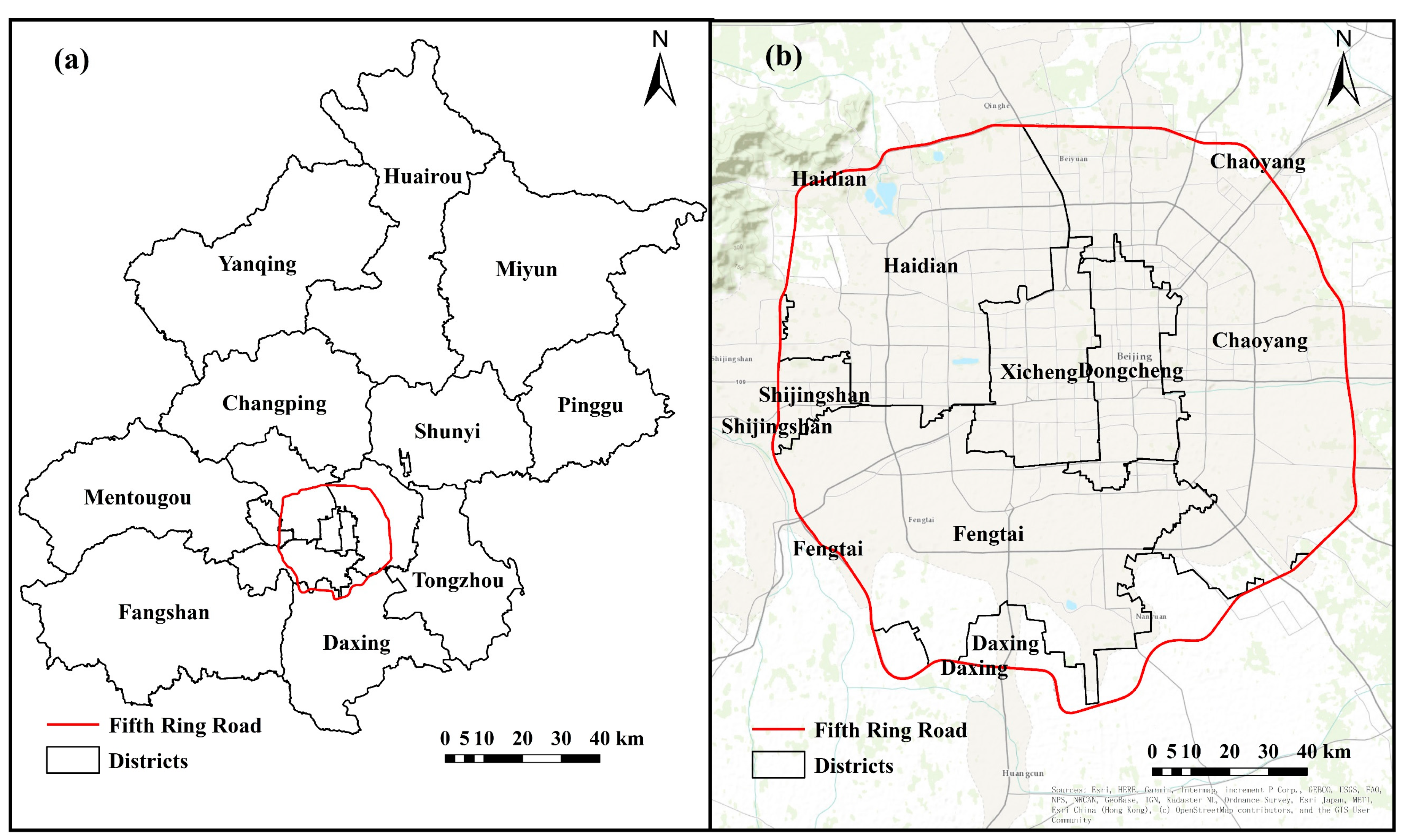
2.1. Study Area

In this paper, we select Beijing as the study area, which is famous as an international metropolis, the capital of China, and a national political center. Beijing is composed of 16 municipal districts and 331 township-level administrative units, covering an area of 16.4 thousand km², with a permanent resident population of more than 21 million in 2019 (Figure 1a). The region within the fifth ring road covers the main urban center of the city (Figure 1b).

2.2. Datasets

2.2.1. Mobile Phone Signaling Data

The mobile phone signaling data in this study were recorded by mobile phone base stations through cell phone signal collection and were obtained from one of the major communication operators in Beijing of China for research purposes. The user ID, longitude and latitude of the mobile phone base station, recording time, and age attributes of the users were recorded when the following events occurred: mobile phone communications, station switching, regular updates, periodic updates, boot, and shutdown [41]. The dataset contained approximately 16 million mobile phone users, which can account for approximately 62% of the mobile phone communication market in Beijing and included mobile phone records on 1 and 6 December 2015 (a weekday and a weekend). There were 20,790 mobile phone base stations extracted from the dataset in Beijing. By calculation, the average distance to the nearest mobile base station was 0.44 km. The average time interval between two successive records was 0.61 h.

2.2.2. POI Data

The POI data of Beijing in 2015 were obtained from a digital mapping company in Beijing of China. The data mainly include 16 POI types and contain 0.38 million points in Beijing. In this paper, we extracted and merged six categories that represent the main POI factors influencing the population distribution during daily life, including accommodation, business, education, restaurant, entertainment and hospital factors. The accommodation factor includes commercial hotels and residential areas. The business factor contains commercial facilities, business services and corporate companies. The education factor includes all kinds of schools and research institutions. The restaurant factor covers a variety of restaurants. The restaurant factor covers a variety of restaurants and the entertainment factor includes leisure resorts and sports buildings. The hospital factor contains the major and community hospitals and medical institutions.

2.2.3. Population Census Data

The population data of the Sixth Population Census conducted on 1 November 2010, were collected from the Beijing Statistical Information Net (http://www.bjstats.gov.cn). The census data are at the street scale, with a total of 315 township-level administrative units across the whole city. The population is presented by age groups, starting at zero, with an age interval of five years. The average area of the subdistrict units is approximately 9.33 km² within the fifth ring road and increases to 86.1 km² beyond the fifth ring road.

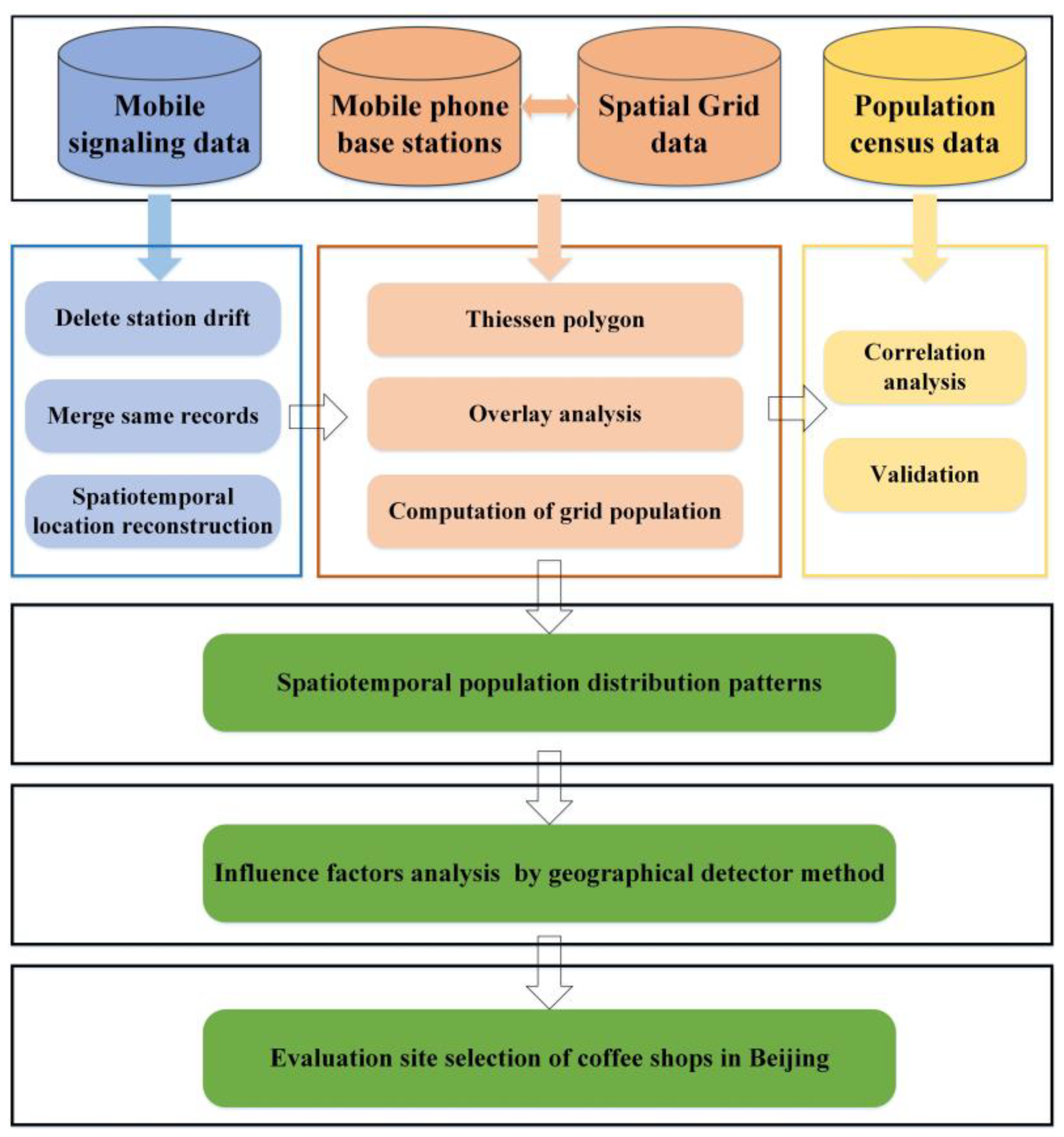
3. Method of Gridding and Validation

The flowchart of the whole framework in this study is shown in Figure 2. The estimation of fine-grained populations of the different age groups is mainly divided into the following three steps. The first step is to reconstruct the spatiotemporal location. Then, the grid population is calculated. Finally, the census data are used to validate the availability of mobile phone location data for population distribution estimation.

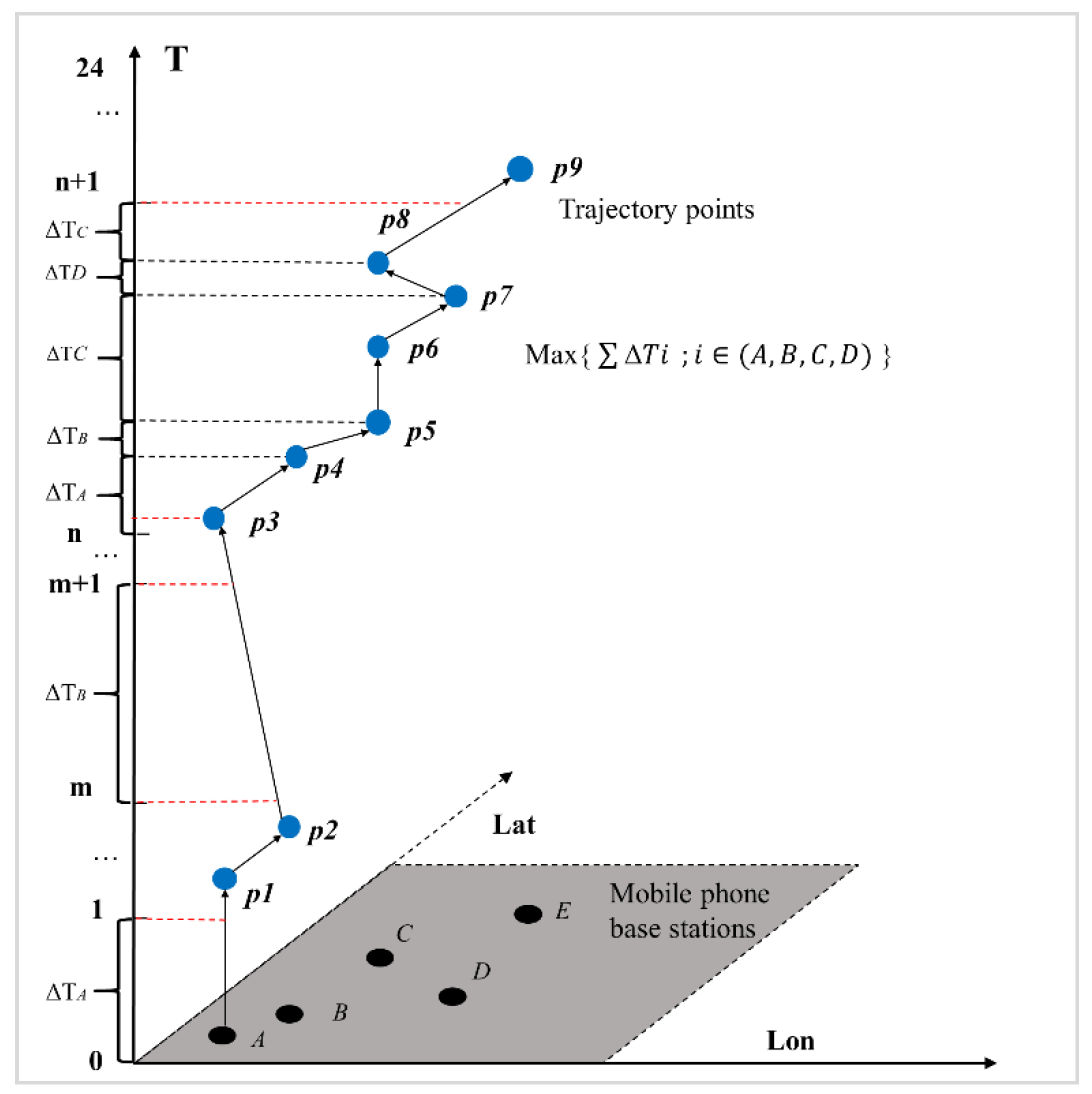
3.1. Reconstruction of the Spatiotemporal Location

Before reconstructing the trajectory, we need to address the station drift issue. This means that users travel from one place to another in a short period of time, but it is impossible to achieve this movement in actual situations. In this study, when the speed of a user passing two successive stations exceeds 50 m/s [42], we assume that station drift exists. In addition, if the position records of the user’s previous point and the next point are the same, we merge the two records into one record and the timestamp is replaced by that of the latter. Given that the average continuous time interval between two records is approximately 0.61 h, we discretize the day into 24 1-h time slots to meet the minimum granularity requirements, and extract a point in each time slot to represent the location of the station where the user stays during that time interval. The spatiotemporal reconstruction algorithm is shown in Figure 3. Processing mainly includes three steps [21,41]: (1) the start time slot, 0 to 1, if there is no record, is filled with the first record of the next nonempty time slot; (2) for periods that have not been recorded, the last record of the last nonempty time slot is selected; (3) if there is at least one record in the time slot, the record is chosen with the longest staying time. Thus far, we can obtain the base location of each user and estimate the population based on each mobile phone base station in each time slot.

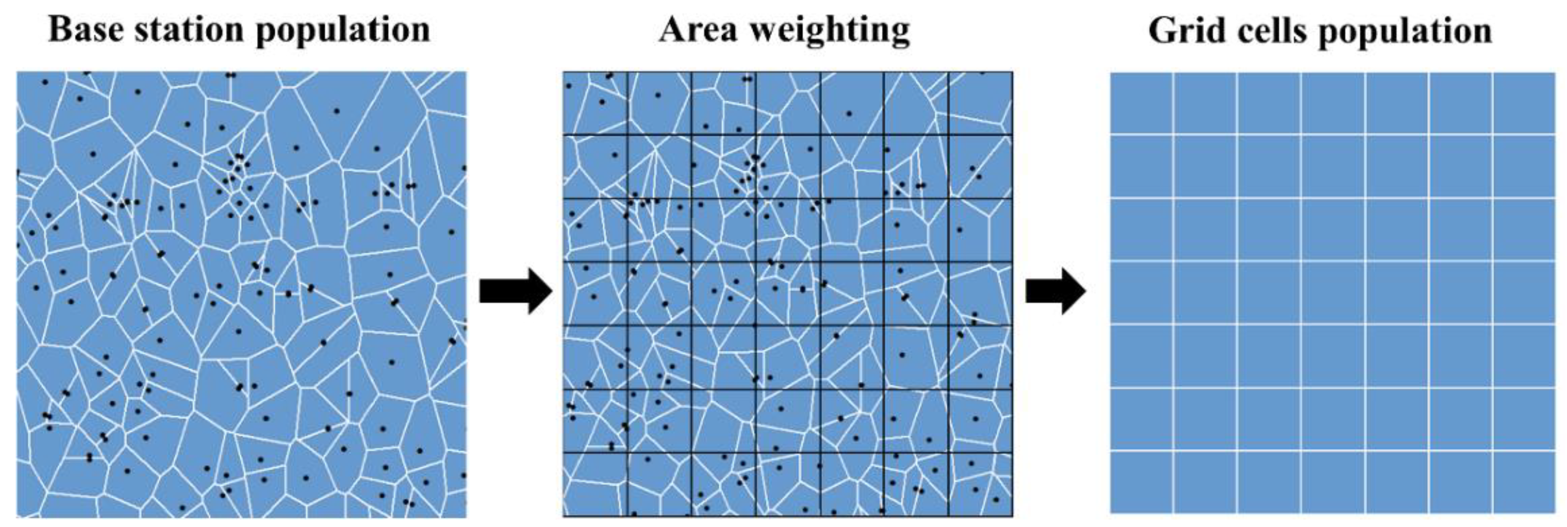
3.2. Computation of the Grid Population

The study area is divided into 500 × 500 m regular grid cells. In this study, we mainly explore the reasons that control the spatial distribution of the population. Therefore, the scale should be as small as possible to reflect the fine-grained population distribution. The mobile phone location data are based on the locations of mobile phone base stations, so the length of cell grid should not be smaller than the distance between base stations [43]. According to calculations and analysis, the average nearest neighbor distance between mobile phone base stations in Beijing is 0.41 km. Hence, a 500 × 500 m grid is a suitable size to reflect the fine-grained population distribution. Moreover, a regular grid can largely eliminate the influence of signal switches between very close mobile phone base stations [44,45]. Next, we redistributed the population based on a mobile phone base station to a regular grid unit. We assume the Thiessen polygon as the service area of the mobile phone base station and removed water areas. The process of population gridding is shown in Figure 4. Thiessen polygons are divided into subunits by regular grids. According to the proportion of the area of each subunit to the total area of the corresponding Thiessen polygon, we can obtain the mobile phone users in each subunit. Then, we calculate the grid population by adding the value of all subunits that fall within the relevant grid. The contribution of this approach is to avoid the situation of void grid population occurring due to there not being any base stations located in that grid.

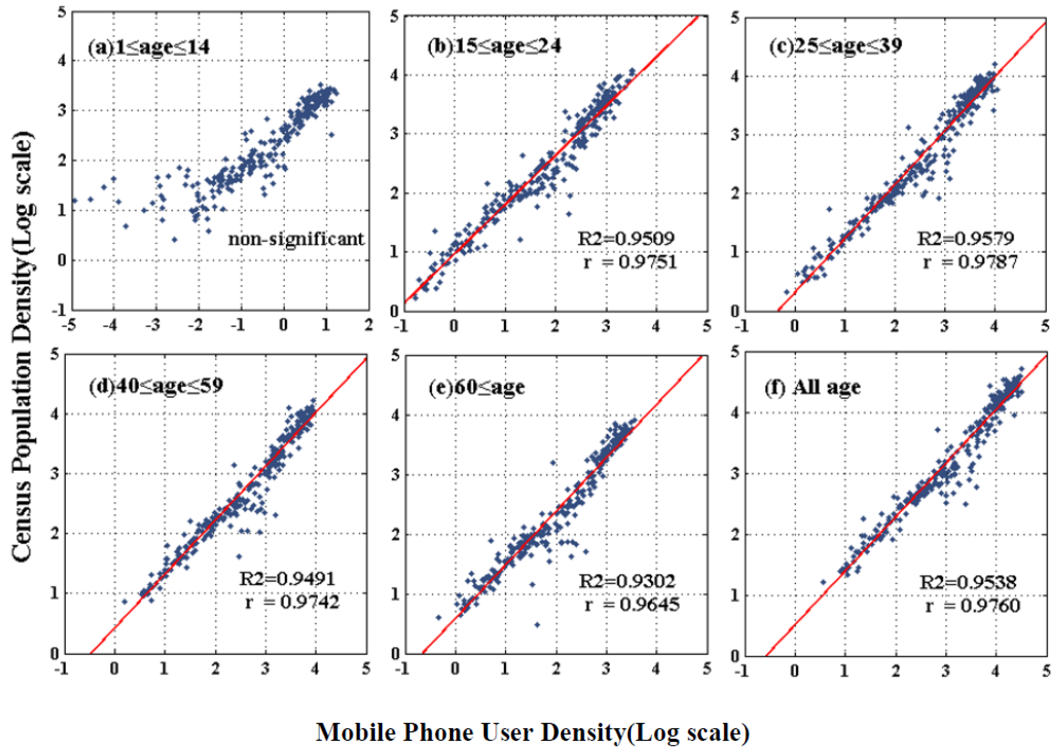
3.3. Validation of the Mobile Location Data Using Population Census Data

We used census data at the subdistrict level to verify the availability of mobile phone location data for population distribution. A total of 294 streets were selected and merged in Beijing to compare the census population density with the density of mobile users at the street scale. The population census data are displayed by age groups, starting at 0, with an interval of 5 years. Therefore, we divided the population into five groups, as shown in Figure 5. Figure 5 shows the result of the log-linear relationship between the nighttime mobile user density and census population density of the different age groups at the subdistrict level. As we can see, there was no significant correlation between the mobile phone user density and census population density for ages 1 to 14 in Figure 5a. The main reason for this result is that the mobile phone ownership rate among the users in this age group is relatively low, resulting in null values in many streets. In Figure 5b–f, significant log-linear relationships exist between the nighttime mobile phone user density and census population density in the other age groups at the subdistrict level. Moreover, the fitting effect is better in the areas with low densities and high-densities mobile phone users. It is clear that the density of mobile phone users is lower than the red line in the medium-density area. Figure 5 also shows the accuracy assessment results using correlation coefficient (r) and determination coefficient (R²). The r value varies between 0.9645 and 0.9787, and the R² value ranges from 0.9302 to 0.9579. The correlation results of the age group of 25 to 39 years were the best, while those of the age group of over 59 years were poorer. Overall, the population density from mobile phone users at night is highly correlated with the census population data except for adolescents, as shown in Figure 5a. Therefore, we mainly analyze the spatiotemporal distributions of adults in further analysis.

4. Population Distribution Patterns in Space and Time

To further study the distribution differences among the different age groups, we divide the mobile phone dataset into the following groups. The people aged 18 to 24 years mainly represent the people in early adulthood. The people aged 25 to 39 years and 40 to 59 years represent young and middle-aged people, respectively. People over 60 years of age represent elderly people because the retirement age in China is 60.

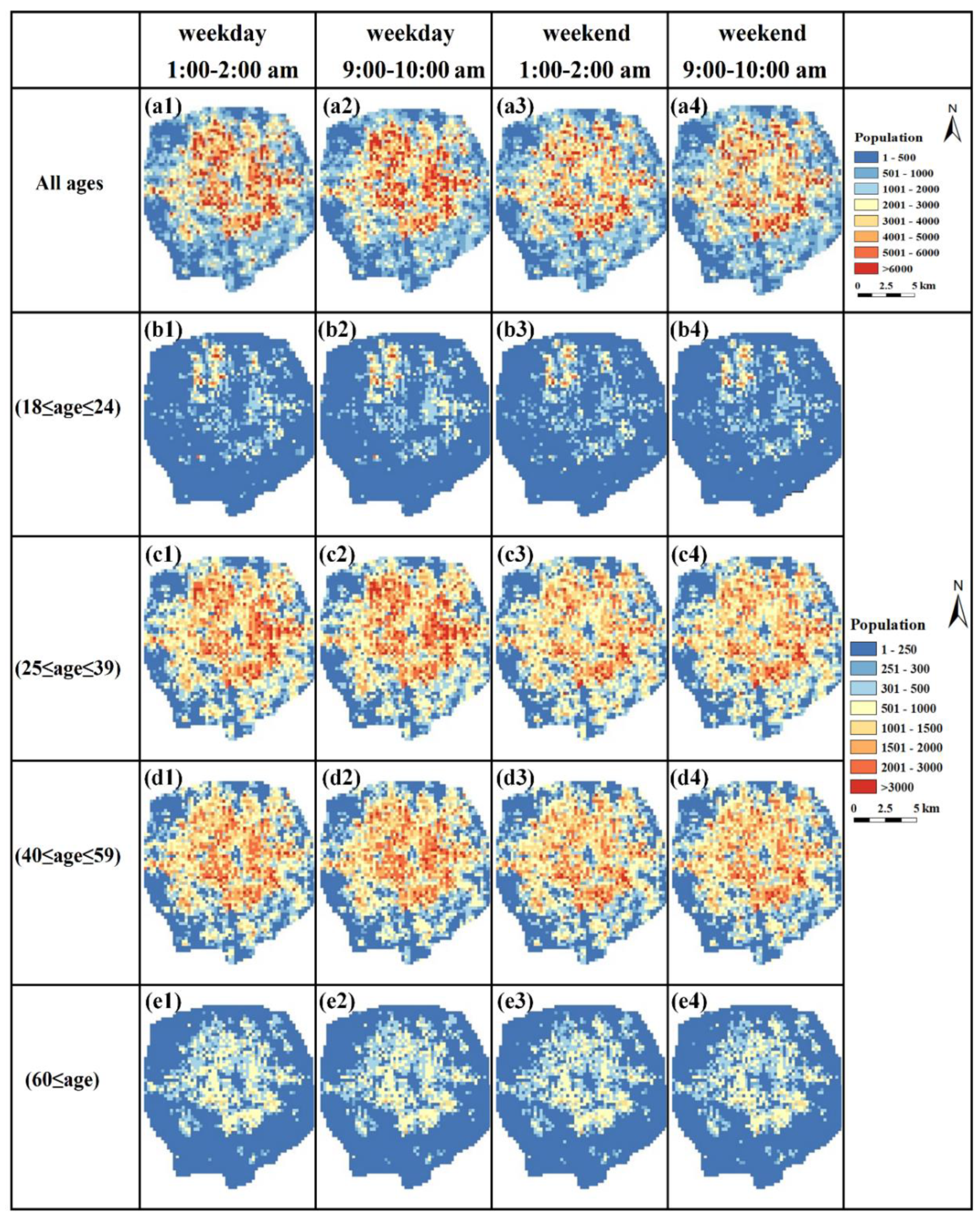
4.1. Spatiotemporal Distribution Characteristics

The spatiotemporal distribution patterns of the populations of the different age groups in the fifth ring road of Beijing in typical time slots are shown in Figure 6. The population distributions over time are displayed in corresponding rows, and each row corresponds to a given age group. When focusing on the entire population distribution in Figure 6a1–a4, we can see that the grids are redder on weekdays than on the weekend. By calculation, the number of people during the daytime increased by 3.1% and 1.7% on weekdays and the weekend, respectively, compared with the number of people at night within the fifth ring road. Grids with a population over 5000 are mainly clustered in the northwest corner, where Zhongguancun is located, which hosts high-tech industrial and university gathering areas; the east corner contains the central business district (CBD). In contrast, the entire population is relatively dispersed on weekends. In particular, the grid population remains high at Beijing’s railway stations. The population density of the central part and the area between the fourth and fifth ring roads is relatively low, corresponding to the Forbidden City area and green spaces, respectively. In Figure 6b1–b4, the early adulthood people are clustered in the northwest teaching areas, such as Tsinghua University, Peking University and many other universities. The early adulthood people exhibit high concentrations in the university area. According to Figure 6c1–c4,d1–d4, the population distributions of young and middle-aged people are similar. To better understand the differences among different age groups, we present the spatial distributions of the different age groups with the highest above-average percentages in Figure 7. Young people exhibit the highest proportion in the areas between the eastern ring roads, and middle-aged people exhibit the highest percentages in the urban centers and western regions. Figure 6e1–e4 shows that elderly people are mainly present between the second and fourth ring roads with little change between weekdays and weekends, and the population density in the south is significantly higher than that in the north, which is consistent with the results shown in Figure 7.

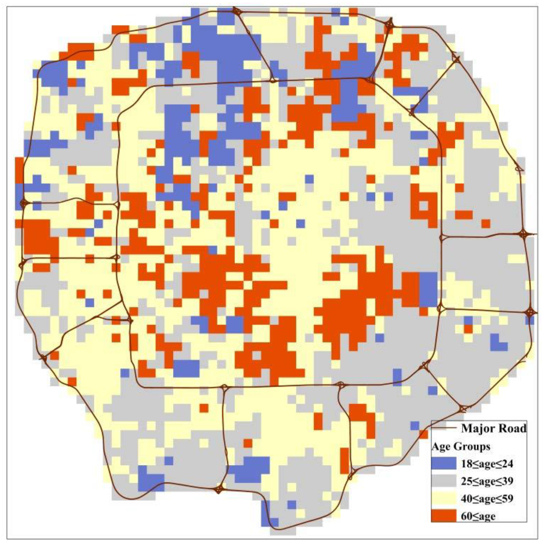
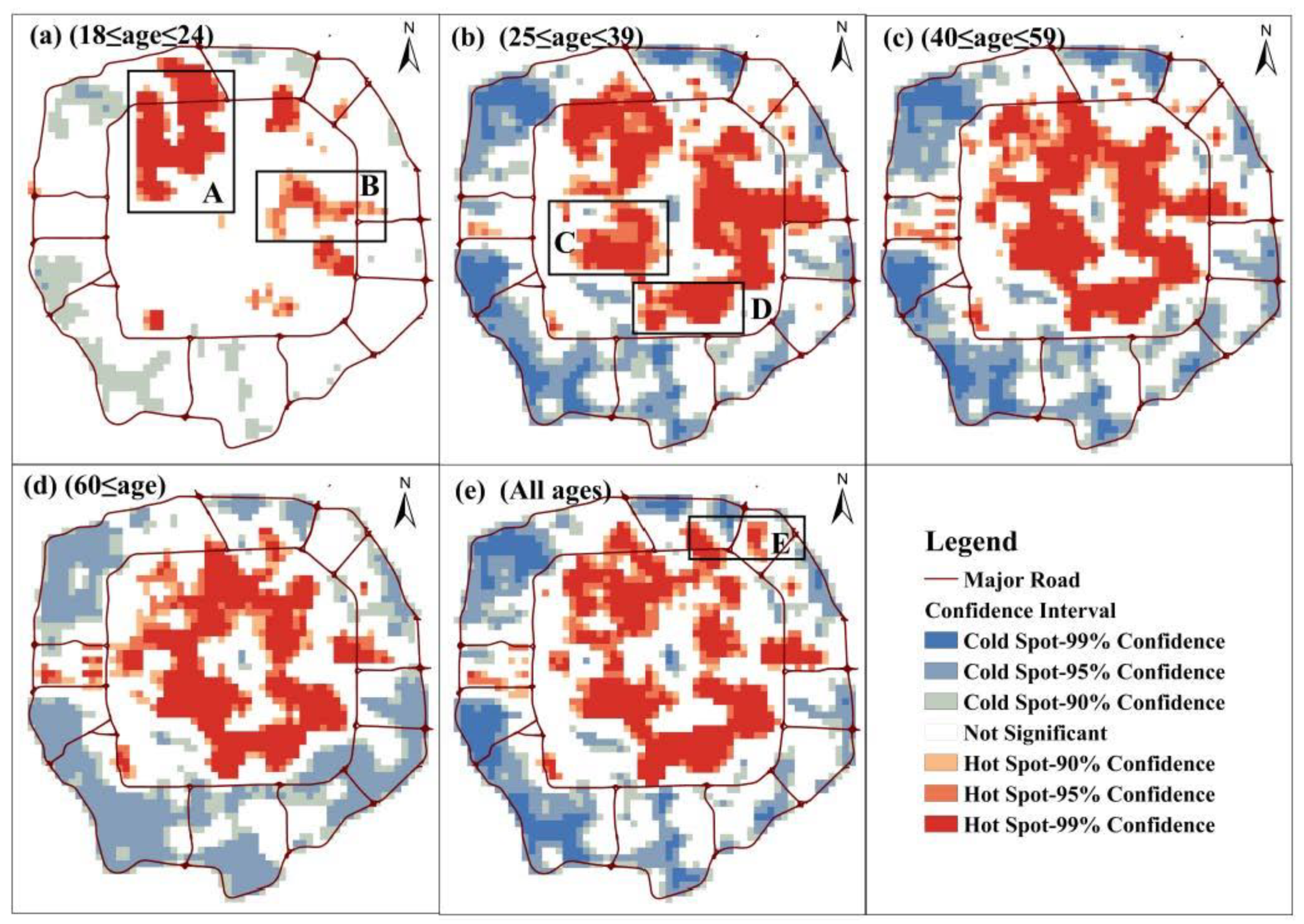
4.2. Spatiotemporal Aggregation

We analyzed the spatiotemporal distribution characteristics of the different age groups. To further explore the distribution differences of the different age groups, we adopt Moran’s I index [46] and the General G index [47] in this study.

Table 1. Spatial autocorrelation analysis results of the grid population using Global Moran’s I for typical time slots.

	18 ≤ Age ≤ 24	25 ≤ Age ≤ 39	40 ≤ Age ≤ 59	60 ≤ Age
1:00–2:00 a.m. weekday	0.4988	0.5472	0.4881	0.5331
1:00–2:00 a.m. weekend	0.5399	0.5851	0.5032	0.5816
9:00–10:00 a.m. weekday	0.5161	0.5819	0.5001	0.5524
9:00–10:00 a.m. weekend	0.5480	0.6088	0.5139	0.5949

shows that the population distribution exhibits a significant positive autocorrelation, which means that the autocorrelation becomes more significant as the spatial location of the population becomes aggregated. The population of 25 to 39 years has the highest autocorrelation, while the population aged 40 to 59 years has the lowest autocorrelation. Moreover, the autocorrelation of the population distribution is more significant during the daytime than at night and more significant on weekdays than on the weekend.

The General G index can represent the specific spatial aggregation patterns of different age distributions, while Moran’s I can reflect only the degree of spatial aggregation of high and low values. Figure 8 shows the spatial aggregation results of the different age groups for a typical time slice. In Figure 8a, we can see that people aged 18 to 24 years are significantly clustered in university gathering areas (region A and other prominent red areas) and central business districts (CBDs) (region B). In Figure 8b, people aged 25 to 39 years are mainly concentrated across several business districts (regions A, B, C, and D) within the fourth ring road. In contrast, the concentration of middle-aged and elderly people in regions A and B is reduced, as shown in Figure 8c,d. For the entire population, according to Figure 8e, the spatial aggregation pattern is similar to that of the age groups, except for people aged 18 to 24 years. At the same time, the Wangjing business district and Asian Sports Village (region E) between the fourth and fifth ring roads exhibit notable population aggregations.

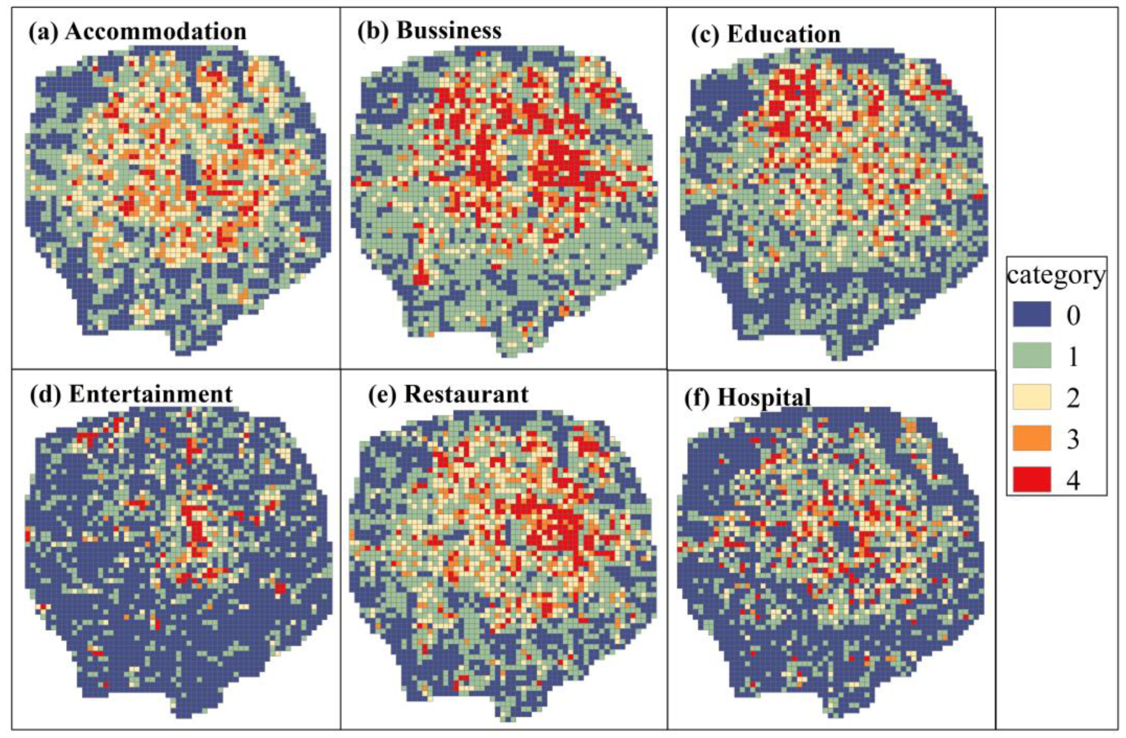
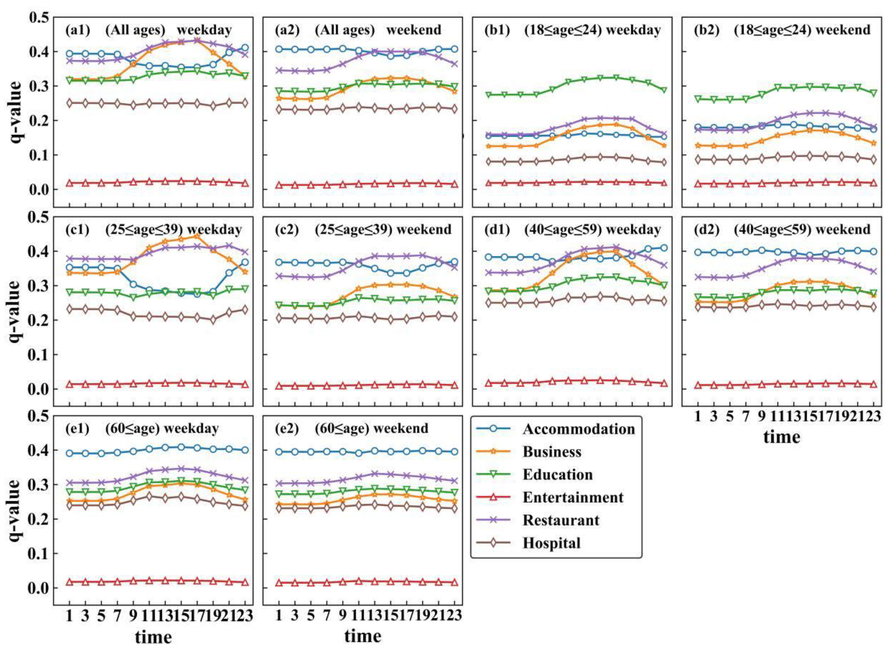
5. Analysis of the Factors Influencing the Population Distribution in Space and Time

We selected the geographic detector method [48,49] to analyze the factors influencing the spatiotemporal population distribution of different age groups using POI data. Geographical detection is a statistical method for detecting spatial heterogeneity and revealing its driving factors, and has become a popular method to interpret the mechanisms of various factors in research studies in many natural and social science fields. The basic idea of the geographical detector relies on the assumption that the study area is divided into several subregions, and if the sum of the variances in the subregions is smaller than the total variance in the entire region, spatially stratified heterogeneity exists. The formula is as follows:

$$q=1-\frac{1}{n{\sigma }^2}{\displaystyle \sum }_{i=1}^m{n}_i{\sigma }_i^2$$

(1)

where q is the factor detector that indicates the degree of a factor explaining the specific attributes, n and ${\sigma }^2$ stand for the number of units and the variance in the regions, respectively, and m is the number of strata. The value range of q is 0 to 1, and the larger the q value is, the stronger the explanatory power is. In this study, the factor detector q-statistic is selected to measure the explanatory power of the POI factor on the population distribution. In addition, the independent variable should be transformed to be categorical if it is numerical. Therefore, we use the equal spacing method to divide the region into five layers according to the number of POI points falling in the corresponding grid. The spatially stratified distributions of six POI factors are shown in Figure 9.

Figure 10 shows the time-series change characteristics of the explanatory power of the different POI factors on the population distributions of the different age groups using the geographical detector. We compared one weekday of 1 December (Figure 10a1–e1) and one weekend day (Figure 10a2–e2) of December 6. Then, the data were analyzed from two aspects of the POI factors influencing the population distributions between the overall population and the different age groups. Figure 10a1,a2 shows the effect of the POI factors on the overall population on weekdays and weekends. Figure 10a1 shows that the accommodation factor plays a major influencing role in the nighttime and that its explanatory power gradually decreases during the daytime, while the explanatory powers of the business and restaurant factors increase and become leading factors. The education and hospital factors remain stable, and the entertainment factor has very little explanatory power. In contrast, Figure 10a2 indicates that the accommodation factor is the main influencing factor throughout the day, while the explanatory power of the restaurant factor declines slightly, and the business factor declined significantly on the weekend. The other factors had similar performances on the weekday. It can be easily explained that crowds are mainly concentrated in residential areas at night and move to work areas and commercial districts during the daytime on weekdays. Historical weather information indicated that winter in Beijing had just started on 6 December 2015, accompanied by light snow. The crowds were mainly concentrated in the residential area throughout the day and less so in the commercial district on the weekend. Because eating is a necessary human activity, the explanatory power of the restaurant factor remains strong on the weekend. Teaching and hospital areas are aimed at small groups, so the explanatory power for the overall population is weak. As expected, the entertainment factor is not the chief activity for people, so the entertainment factor has little effect on the population distribution.

When the population is divided into different age groups, we can explore the effect of POI factors on the distribution of different groups. In general, the influence of factors on the distributions of different age groups is significantly different. According to Figure 10b1,b2, the education factor has a stronger explanatory power for the people aged 18–24 years old than the other POI factors, and there is no significant difference between weekdays and weekends. The explanatory powers of the business and restaurant factors show a slight upward trend during the daytime, while that of the accommodation factor remains steady. The main reason for this difference is that most of this age group are college students who are distributed across the teaching districts.

According to Figure 10c1,c2, the main factors influencing the distribution of people aged 25–39 years are accommodation, business, and restaurant factors. In particular, the explanatory power of the business factor increased significantly and that of the accommodation factor sharply decreased during the daytime on the weekday. It can be inferred that an obvious separation of occupation and residence exists among young people on the weekday. In contrast, the explanatory power of the accommodation factor decreases slightly during the daytime, and that of the business factor declines as a whole on the weekend. Moreover, the explanatory power of the restaurant factor for young people is highest at night on the weekday and during the day on the weekend. This result suggests that the food-related activities of young people are still frequent on weeknights and weekends.

Figure 10d1,d2 shows the detection results for people aged 40 to 59 years, which are significantly different from those for young people. The explanatory power of the accommodation factor slightly decreased, and the explanatory power of the restaurant factor was higher than that of the business factor during the daytime on weekdays. It may be inferred that middle-aged people with a good economic foundation have higher freedom of life and fewer constraints of commuting. In addition, the explanatory power of the restaurant factor has always been lower than that of the accommodation factor on the weekend. This result indicates that middle-aged people have lower food-related activity intensity on the weekend and are more likely to eat at home compared with young people.

According to Figure 10e1,e2, the most powerful explanation factor for elderly people is the accommodation factor for both weekdays and weekends. It can be explained that elderly people who are retired and have minimal activity intensity are concentrated in the residential area. In addition, the hospital factor has the highest explanatory power for elderly people, and the explanatory power increases slightly during the day on weekdays. Specifically, the entertainment factors have very little explanatory power for the population distributions of the different age groups. By subdividing the population, we can obtain detailed characteristics of the influence of factors on the distribution of different age groups, which provides a better understanding of the differences of different age groups.

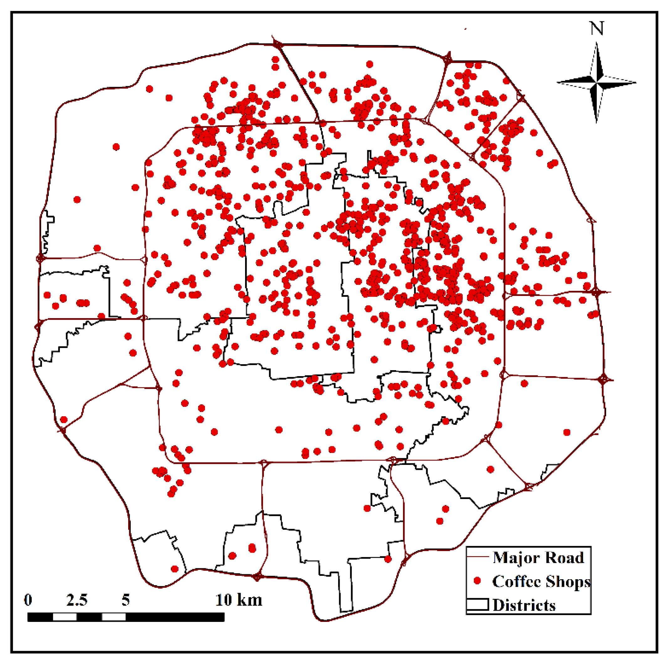
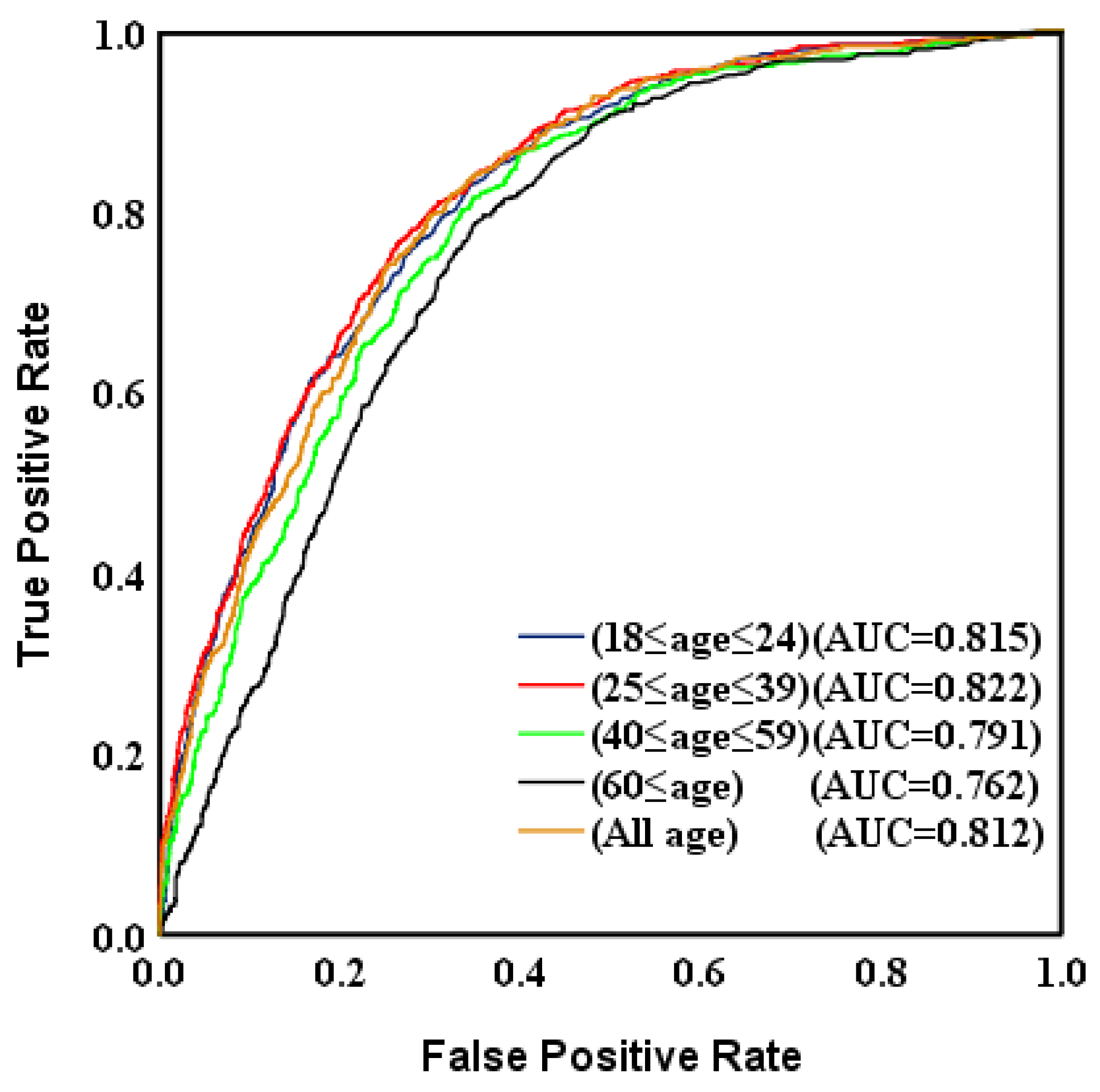
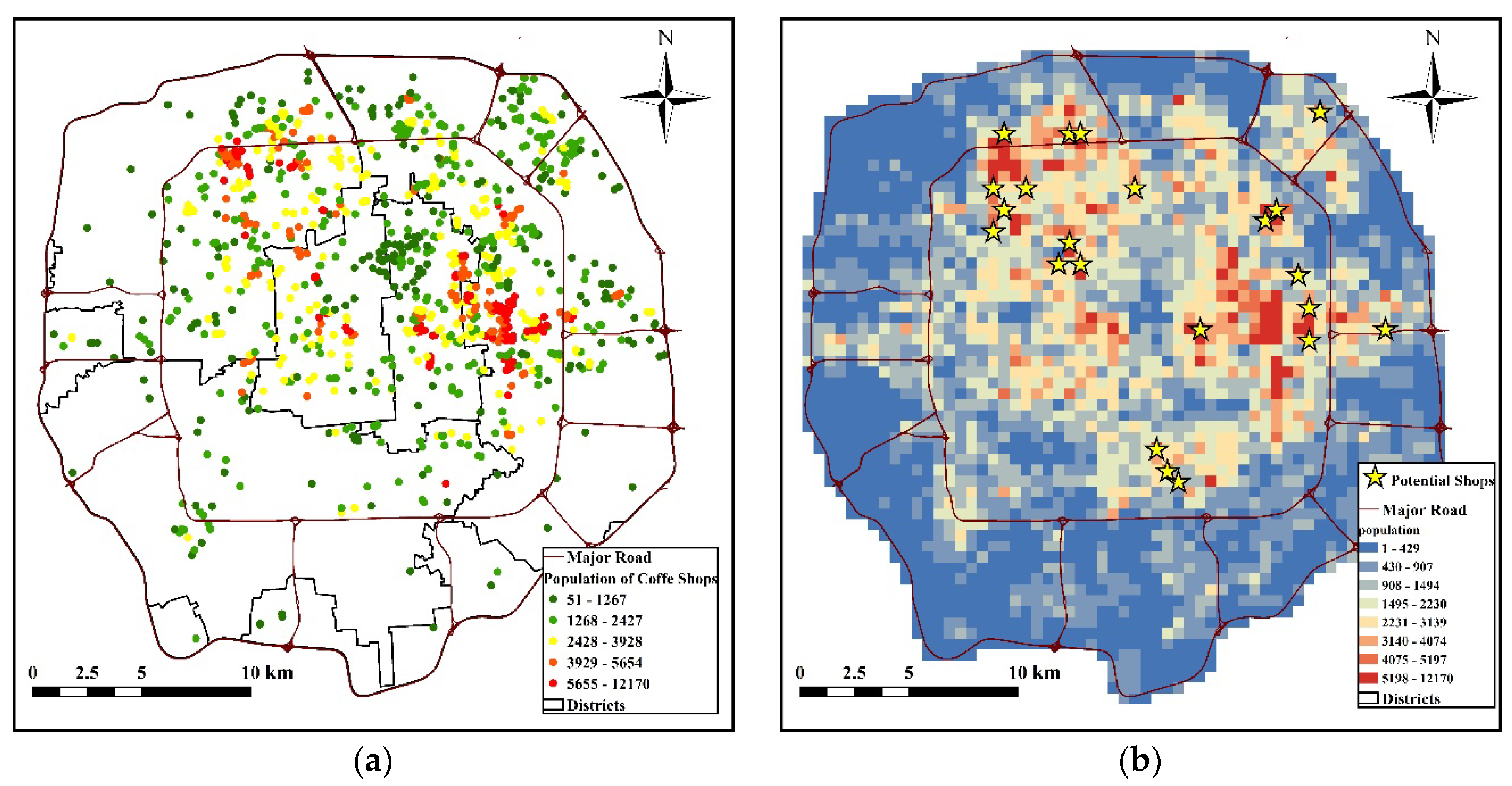
6. Evaluation Site Selection of Coffee Shops in Beijing

In this study, to verify the importance of the fined-grained population of the different age groups in the selection of an urban business location, we used mobile phone population data during meal time (12:00–13:00) to evaluate the locations of coffee shops in Beijing. By analyzing the correlation between the coffee shop locations and population distributions of the different age groups, it was shown that the coffee shop locations were highly related to age. Therefore, we can provide guidance on the locations of potential stores using the fine-grained population data for the different age groups. Figure 11 shows the spatial distribution of coffee shops in the fifth ring road of Beijing, where the red dots represent coffee shops. The coffee shops are mainly located in the northwest and northeast of the downtown area.

For quantitative analysis of the correlation between the coffee shop locations and population distributions of the different age groups, the following methods are adopted: Spearman’s correlation coefficient and univariate and multivariate logistic regression. We assume that the dependent variable is a binary variable, which indicates whether a coffee shop is present in the corresponding grid, and the grid population is the independent variable. To avoid excessively small coefficients, the grid population unit is expressed per thousand people. First, correlation analysis of the independent and dependent variables is performed. Because the independent and dependent variables do not conform to the normal distribution, we calculate the Spearman correlation coefficient in this paper. Next, a logistic regression is performed for the percentage of correctly classified points for the different age groups, and the receiver operating characteristic (ROC) test is conducted. The results of the Spearman correlation coefficient and logistic regression of the correct percentage are listed in

Table 2. Spearman correlation coefficient and logistic regression of correct percentage for the different age groups.

	Spearman Correlation Coefficient	Correct Percentage
All age	0.4418	81.10
18 ≤ age ≤ 24	0.4456	80.86
25 ≤ age ≤ 39	0.4562	81.61
40 ≤ age ≤ 59	0.4124	79.75
60 ≤ age	0.3706	78.82

, and the ROC curves and area under the curve (AUC) values are displayed in Figure 12. A significant correlation between the independent and dependent variables is shown in Table 2. The correlation coefficient of people aged 25–39 years reaches a maximum of 0.4562, and that of people over 60 years reaches a minimum of 0.3706. Similarly, the logistic regression of people aged 25 to 39 years has the highest correct classification percentage, with a value of 81.61%, and people over 60 years have the lowest correct classification percentage, with a value of 78.82%.

Then, multivariate logistic regression was used to analyze the correlations among the different age groups further. The results of logistic regression include regression coefficients, standard errors, Wald statistics, degrees of freedom, the significance level, EXP (β), and confidence intervals of EXP (β).

Table 3. Multivariate logistic regression between the population distributions of the different age groups and locations of coffee shops within the fifth ring road of Beijing.

	B	SE	Wald	df	P	EXP (β)	95% Confidence Interval of EXP (β)
							Lower	Upper
18 ≤ age ≤ 24	0.552	0.226	5.942	1	0.015	1.736	1.114	2.706
25 ≤ age ≤ 39	1.522	0.175	75.829	1	0.000	4.582	3.253	6.454
40 ≤ age ≤ 59	−0.621	0.302	4.226	1	0.040	0.537	0.279	0.972
60 ≤ age	0.137	0.538	0.065	1	0.799	1.147	0.399	3.294
constant	−2.656	0.092	828.299	1	0.000	0.070

shows the regression results of the different age groups as multiple independent variables. The regression coefficients show that the groups aged 18 to 24 years and aged 25 to 39 years are positively correlated with the coffee shop locations. In contrast, the group aged 40 to 59 years displays a negative correlation. There was no statistically significant correlation between the coffee shop location and people over 59 years old at a significance level of 0.799. We can see that the regression coefficient of the people aged 25–39 years reaches a maximum of 1.522 with a significance less than 0.01. When the number of people increases by 1000, the probability of someone aged 25 to 39 years being at a coffee shop in the grid increases by 152%, and the probability of someone 40–59 years being at a coffee shop in the grid decreases by 62.1%.

The grid population of ages 18–39 owning coffee shops is shown in Figure 13a, where the red dots represent the coffee shops with a large grid population. The red dots are mainly concentrated in the business districts, such as Zhongguancun and Suzhou Street in the northwest, the eastern CBD region, and the Wangfujing and Xidan districts in the urban centers. Moreover, coffee shops also present at certain scenic spots with small grid populations, such as Gulou Street. The main reason is that the day that was analyzed is a winter working day, so the populations at the scenic areas are small. Finally, we use the fine-grained population aged 18–39 years to select potential shop locations. Considering the competition of existing coffee shops, we choose grids without coffee shops and more than 3000 people as potential location grids, as shown in Figure 13b. At the actual business location, population size is only one important factor, and we should consider other factors, such as shop rent and environmental factors.

7. Conclusions and Discussions

This study constructed a framework to generate fine-grained population data for different age groups based on mobile phone data, which contributes to mapping the hourly population distributions of different age groups. We take Beijing as an example to analyze the distribution patterns of different age groups. The results indicate that there are significant differences in the spatial distribution among different age groups. Early adulthood people are clustered in the northwest corner, where universities are mainly concentrated. Unexpectedly, we found that this age group also showed a significant clustering pattern in the eastern business district area. We found that the distribution and aggregation patterns of young people and middle-aged people within the fifth ring road of Beijing were basically consistent with the distributions of business districts. Elderly people were highly concentrated within the second and fourth ring roads, and the concentration of elderly people was higher in the south than in the north.

We explored the effect of different factors on the dynamic changes in the population distribution of different age groups. The following conclusions were drawn. The education factor is the most powerful exploratory factor for the distribution of early adulthood people. Business, restaurant and accommodation factors were the main factors influencing the population distributions of young and middle-aged people. Further, we found that the separation of occupation and residence was particularly obvious for young people. This result occurred because the explanatory power of the business factor increased significantly and that of the accommodation factor sharply decreased during the day on weekdays. We also found that the restaurant factor had the greatest influence on the distribution of young people. The explanatory power of the restaurant factor for young people was the highest at night on weekdays and during the day on weekends. As expected, the accommodation factor had a major influence on the distribution of elderly people. Moreover, the hospital factor had a strong effect on the distribution of elderly people. Specifically, the entertainment factor had very little explanatory power for the population distributions of the different age groups.

To embrace the achievements of fine-grained population data of different age groups in this study, we suggest that city managers should fully consider the distribution differences of different age groups and provide corresponding services for different age groups, such as the allocation of infrastructure for elderly people, child-friendly community planning, and new stores (e.g., coffee shops) for young people. However, this study still has deficiencies. First, the mobile signaling data used in this article are from a single communication operator and cannot represent the distribution of the entire population, as only two days are covered. Second, when spatial partitioning is carried out with the geographical detector method, we assume that the weights of the different POIs in one category remain the same. Future work will focus on these issues. We will consider the weighting of different POIs and combine other data sources (e.g., land use types) to further the analysis of influencing factors. Moreover, the findings on the influencing factors will help to improve our ability to predict more reliable fine-grained distributions of different age groups in space and time.

References

1. Guo, S.; Song, C.; Pei, T.; Liu, Y.; Ma, T.; Du, Y.; Chen, J.; Fan, Z.; Tang, X.; Peng, Y. Accessibility to urban parks for elderly residents: Perspectives from mobile phone data. Landsc. Urban Plan. 2019, 191, 103642. [Google Scholar] [CrossRef]
2. Reyes, M.; Páez, A.; Morency, C. Walking accessibility to urban parks by children: A case study of Montreal. Landsc. Urban Plan. 2014, 125, 38–47. [Google Scholar] [CrossRef]
3. Mokrysz, S. Consumer preferences and behaviour on the coffee market in Poland. Forum Sci. Oecon. 2016, 4, 91–108. [Google Scholar]
4. Sugiyama, T.; Thompson, C.W. Associations between characteristics of neighbourhood open space and older people’s walking. Urban For. Urban Green. 2008, 7, 41–51. [Google Scholar] [CrossRef]
5. Wu, S.-S.; Qiu, X.; Wang, L. Population Estimation Methods in GIS and Remote Sensing: A Review. Mapp. Sci. Remote Sens. 2005, 42, 80–96. [Google Scholar] [CrossRef]
6. Deichmann, U.; Balk, D.; Yetman, G. Transforming Population Data for Interdisciplinary Usages: From Census to Grid. In Population Health Metrics-Popul Health Metrics; Center for International Earth Science Information Network: Washington, DC, USA, 2001. [Google Scholar]
7. Balk, D.; Yetman, G. The Global Distribution of Population: Evaluating the Gains in Resolution Refinement; Center for International Earth Science Information Network (CIESIN), Columbia University: New York, NY, USA, 2004. [Google Scholar]
8. Balk, D.; Deichmann, U.; Yetman, G.; Pozzi, F.; Hay, S.; Nelson, A. Determining global population distribution: Methods, applications and data. Adv. Parasitol. 2006, 62, 119–156. [Google Scholar]
9. Jia, P.; Qiu, Y.; Gaughan, A.E. A fine-scale spatial population distribution on the high-resolution gridded population surface and application in Alachua County, Florida. Appl. Geogr. 2014, 50, 99–107. [Google Scholar] [CrossRef]
10. Reed, F.; Gaughan, A.; Stevens, F.; Yetman, G.; Sorichetta, A.; Tatem, A. Gridded population maps informed by different built settlement products. Data 2018, 3, 33. [Google Scholar] [CrossRef] [Green Version]
11. Bakillah, M.; Liang, S.; Mobasheri, A.; Jokar Arsanjani, J.; Zipf, A. Fine-resolution population mapping using OpenStreetMap points-of-interest. Int. J. Geogr. Inf. Sci. 2014, 28, 1940–1963. [Google Scholar] [CrossRef]
12. Stevens, F.R.; Gaughan, A.E.; Linard, C.; Tatem, A.J. Disaggregating census data for population mapping using random forests with remotely-sensed and ancillary data. PLoS ONE 2015, 10, e0107042. [Google Scholar] [CrossRef] [Green Version]
13. Pei, T.; Sobolevsky, S.; Ratti, C.; Shaw, S.-L.; Li, T.; Zhou, C. A new insight into land use classification based on aggregated mobile phone data. Int. J. Geogr. Inf. Sci. 2014, 28, 1988–2007. [Google Scholar] [CrossRef] [Green Version]
14. Agard, B.; Morency, C.; Trépanier, M. Mining public transport user behaviour from smart card data. IFAC Proc. Vol. 2006, 39, 399–404. [Google Scholar] [CrossRef]
15. Meneses, F.; Moreira, A. Large scale movement analysis from WiFi based location data. In Proceedings of the 2012 International Conference on Indoor Positioning and Indoor Navigation (IPIN), Sydney, Australia, 13–15 November 2012; pp. 1–9. [Google Scholar]
16. Yuan, J.; Zheng, Y.; Zhang, C.; Xie, W.; Xie, X.; Sun, G.; Huang, Y. T-drive: Driving directions based on taxi trajectories. In Proceedings of the 18th SIGSPATIAL International Conference on Advances in Geographic Information Systems, San Jose, CA, USA, 2–5 November 2010; pp. 99–108. [Google Scholar]
17. Liu, Y.; Liu, X.; Gao, S.; Gong, L.; Kang, C.; Zhi, Y.; Chi, G.; Shi, L. Social sensing: A new approach to understanding our socioeconomic environments. Ann. Assoc. Am. Geogr. 2015, 105, 512–530. [Google Scholar] [CrossRef]
18. Yue, Y.; Lan, T.; Yeh, A.G.O.; Li, Q.Q. Zooming into individuals to understand the collective: A review of trajectory-based travel behaviour studies. Travel Behav. Soc. 2014, 1, 69–78. [Google Scholar] [CrossRef]
19. Xu, F.; Zhang, P.; Li, Y. Context-aware real-time population estimation for metropolis. In Proceedings of the 2016 ACM International Joint Conference on Pervasive and Ubiquitous Computing, Heidelberg, Germany, 12–16 Sepetmber 2016; pp. 1064–1075. [Google Scholar]
20. Candia, J.; González, M.C.; Wang, P.; Schoenharl, T.; Madey, G.; Barabási, A.-L. Uncovering individual and collective human dynamics from mobile phone records. J. Phys. A Math. Theor. 2008, 41, 224015. [Google Scholar] [CrossRef] [Green Version]
21. Chen, J.; Pei, T.; Shaw, S.-L.; Lu, F.; Li, M.; Cheng, S.; Liu, X.; Zhang, H. Fine-grained prediction of urban population using mobile phone location data. Int. J. Geogr. Inf. Sci. 2018, 32, 1770–1786. [Google Scholar] [CrossRef]
22. Kang, C.; Liu, Y.; Ma, X.; Wu, L. Towards Estimating Urban Population Distributions from Mobile Call Data. J. Urban Technol. 2012, 19, 3–21. [Google Scholar] [CrossRef]
23. Ratti, C.; Pulselli, R.M.; Williams, S.; Frenchman, D. Mobile Landscapes: Using location data from cell phones for urban analysis. Environ. Plan. B Plan. Des. 2006, 33, 727–748. [Google Scholar] [CrossRef]
24. Reades, J.; Calabrese, F.; Ratti, C. Eigenplaces: Analysing cities using the space-time structure of the mobile phone network. Environ. Plan. B Plan. Des. 2009, 36, 824–836. [Google Scholar] [CrossRef] [Green Version]
25. Krings, G.; Calabrese, F.; Ratti, C.; Blondel, V.D. Urban gravity: A model for inter-city telecommunication flows. J. Stat. Mech. Theory Exp. 2009, 2009, L07003. [Google Scholar] [CrossRef] [Green Version]
26. Pierre, D.; Catherine, L.; Samuel, M.; Marius, G.; Stevens, F.R.; Gaughan, A.E.; Blondel, V.D.; Tatem, A.J. Dynamic population mapping using mobile phone data. Proc. Natl. Acad. Sci. USA 2014, 111, 15888–15893. [Google Scholar]
27. Liu, Z.; Ma, T.; Du, Y.; Pei, T.; Yi, J.; Peng, H. Mapping hourly dynamics of urban population using trajectories reconstructed from mobile phone records. Trans. GIS 2018, 22, 494–513. [Google Scholar] [CrossRef]
28. Kwan, M.P. Gender differences in space-time constraints. Area 2000, 32, 145–156. [Google Scholar] [CrossRef]
29. Zhou, S.; Yang, L.; Deng, L. The Spatial-Temporal Pattern of People’s Daily Activities and Transportation Demand Analysis-A Case Study of Guangzhou, China. In Proceedings of the 2010 International Conference on Management and Service Science, Wuhan, China, 24–26 August 2010; pp. 1–4. [Google Scholar]
30. Dai, D.; Zhou, C.; Ye, C. Spatial-temporal characteristics and factors influencing commuting activities of middle-class residents in Guangzhou City, China. Chin. Geogr. Sci. 2016, 26, 410–428. [Google Scholar] [CrossRef] [Green Version]
31. Plotnikoff, R.C.; Mayhew, A.; Birkett, N.; Loucaides, C.A.; Fodor, G. Age, gender, and urban-rural differences in the correlates of physical activity. Prev. Med. 2004, 39, 1115–1125. [Google Scholar] [CrossRef] [PubMed]
32. Van Tuyckom, C.; Scheerder, J.; Bracke, P. Gender and age inequalities in regular sports participation: A cross-national study of 25 European countries. J. Sports Sci. 2010, 28, 1077–1084. [Google Scholar] [CrossRef] [PubMed]
33. Karagel, D.Ü. The distribution of elderly population in Turkey and the factors effecting this distribution. Int. J. Soc. Sci. Hum. Stud. 2011, 3, 59–69. [Google Scholar]
34. Zhou, J.; Chai, Y. Research progress on spatial behaviors of the elderly in China. Prog. Geogr. 2013, 32, 722–732. [Google Scholar]
35. Zhou, S.; Xie, M.; Kwan, M.-P. Ageing in place and ageing with migration in the transitional context of urban China: A case study of ageing communities in Guangzhou. Habitat Int. 2015, 49, 177–186. [Google Scholar] [CrossRef]
36. Atkins, M.T.; Tonts, M. Exploring Cities through a Population Ageing Matrix: A spatial and temporal analysis of older adult population trends in Perth, Australia. Aust. Geogr. 2016, 47, 65–87. [Google Scholar] [CrossRef]
37. Scheiner, J.; Huber, O.; Lohmüller, S. Children’s mode choice for trips to primary school: A case study in German suburbia. Travel Behav. Soc. 2019, 15, 15–27. [Google Scholar] [CrossRef]
38. Yoon, S.Y.; Doudnikoff, M.; Goulias, K.G. Spatial analysis of propensity to escort children to school in southern California. Transp. Res. Rec. 2011, 2230, 132–142. [Google Scholar] [CrossRef]
39. Sidharthan, R.; Bhat, C.R.; Pendyala, R.M.; Goulias, K.G. Model for children’s school travel mode choice: Accounting for effects of spatial and social interaction. Transp. Res. Rec. 2011, 2213, 78–86. [Google Scholar] [CrossRef] [Green Version]
40. Yuan, Y.; Raubal, M.; Liu, Y. Correlating mobile phone usage and travel behavior—A case study of Harbin, China. Comput. Environ. Urban Syst. 2012, 36, 118–130. [Google Scholar] [CrossRef]
41. Xu, Y.; Shaw, S.-L.; Lu, F.; Chen, J.; Li, Q. Uncovering the relationships between phone communication activities and spatiotemporal distribution of mobile phone users. In Human Dynamics Research in Smart and Connected Communities; Springer: Berlin/Heidelberg, Germany, 2018; pp. 41–65. [Google Scholar]
42. Fan, Z.; Tao, P.; Ma, T.; Du, Y.; Song, C.; Zhang, L.; Zhou, C. Estimation of urban crowd flux based on mobile phone location data: A case study of Beijing, China. Comput. Environ. Urban Syst. 2018, 69, 114–123. [Google Scholar] [CrossRef]
43. Kang, C.; Sobolevsky, S.; Liu, Y.; Ratti, C. Exploring human movements in Singapore: A comparative analysis based on mobile phone and taxicab usages. In Proceedings of the 2nd ACM SIGKDD International Workshop on Urban Computing, Chicago, IL, USA, 11 August 2013; p. 1. [Google Scholar]
44. Xu, Y.; Shaw, S.-L.; Zhao, Z.; Yin, L.; Lu, F.; Chen, J.; Fang, Z.; Li, Q. Another tale of two cities: Understanding human activity space using actively tracked cellphone location data. Ann. Am. Assoc. Geogr. 2016, 106, 489–502. [Google Scholar]
45. Yang, X.; Fang, Z.; Yang, X.; Shaw, S.L.; Zhao, Z.; Ling, Y.; Tao, Z.; Lin, Y. Understanding Spatiotemporal Patterns of Human Convergence and Divergence Using Mobile Phone Location Data. ISPRS Int. J. Geo-Inf. 2016, 5, 177. [Google Scholar] [CrossRef]
46. Moran, P.A. Notes on continuous stochastic phenomena. Biometrika 1950, 37, 17–23. [Google Scholar] [CrossRef]
47. Getis, A.; Ord, J.K. The analysis of spatial association by use of distance statistics. In Perspectives on Spatial Data Analysis; Springer: Berlin/Heidelberg, Germany, 2010; pp. 127–145. [Google Scholar]
48. Wang, J.F.; Li, X.H.; Christakos, G.; Liao, Y.L.; Zhang, T.; Gu, X.; Zheng, X.Y. Geographical detectors-based health risk assessment and its application in the neural tube defects study of the Heshun Region, China. Int. J. Geogr. Inf. Sci. 2010, 24, 107–127. [Google Scholar] [CrossRef]
49. Wang, J.; Xu, C. Geodetector: Principle and prospective. Acta Geogr. Sin. 2017, 72, 116–134. [Google Scholar]
Figure 1. (a) The municipal districts of Beijing; (b) the central region within the fifth ring road of Beijing.
Sustainability 11 07033 g001
Figure 2. Framework of population distribution estimation and analysis.
Sustainability 11 07033 g002
Figure 3. Reconstruction algorithm of the spatiotemporal location.
Sustainability 11 07033 g003
Figure 4. The process of population gridding.
Sustainability 11 07033 g004
Figure 5. The log-linear relationship between the nighttime mobile user density and population census density of the different age groups at the subdistrict level. The red line shows the fitting result curve, and r and R2 represent the correlation coefficient and coefficient of determination, respectively.
Sustainability 11 07033 g005
Figure 6. The spatiotemporal grid population distributions of the different age groups in the central region within the fifth ring road of Beijing.
Sustainability 11 07033 g006
Figure 7. The spatial distributions of the different age groups with the highest above-average percentages.
Sustainability 11 07033 g007
Figure 8. The spatial aggregation patterns of the grid population using the general G index from 9:00–10:00 on 1 December. Regions A, B, C, D and E are the Zhongguancun business district, CBD business district, Xidan business district, Muxiyuan district, Wangjing business district and Asian Sports Village, respectively.
Sustainability 11 07033 g008
Figure 9. The spatially stratified distributions of six POI factors.
Sustainability 11 07033 g009
Figure 10. Dynamic changes in the explanatory power of POI factors on population distribution for different age groups. The time on the x-axis is represented in the 24-h system.
Sustainability 11 07033 g010
Figure 11. The spatial distribution of the coffee shops in the fifth ring road of Beijing.
Sustainability 11 07033 g011
Figure 12. Logistic regression ROC curves and AUC values.
Sustainability 11 07033 g012
Figure 13. (a) Coffee shop distribution with the grid population aged 18 to 39 years and (b) the potential shop locations.
Sustainability 11 07033 g013