Abstract
Ozone is an important secondary air pollutant and plays different significant roles in regulating the formation of secondary organic aerosols. However, the characteristics of winter vertical ozone distributions have rarely been studied. In the winter of 2017, field experiments were performed in Shanghai, China using hexacopter unmanned aerial vehicle (UAV) platforms. The vertical profiles of ozone were obtained from 0–1200 m above the ground level. Results show that the UAV observations were reliable to capture the vertical variations of ozone. Vertical ozone profiles in the winter are classified into four categories: (1) well-mixed profile, (2) altitudinal increasing profile, (3) stratification profile, and (4) spike profile. Results show that although the average surface ozone level was relatively low, strong ozone variability and high ozone concentrations occurred at the upper air. The maximum observed ozone concentration was 220 ppb. In addition, using meteorological profiles and backward trajectories, we found that the ozone elevation aloft can be attributed to the downward transport of air flow from higher altitudes. Furthermore, ozone accumulation in the winter could be influenced by the horizontal transport of air masses for the northern part of China. This study successfully used hexacopter UAV platforms to perform vertical observations within the boundary layer. This provides systematic classification of winter ozone distribution within the boundary layer.
1. Introduction
In many regions around the world, especially in developed cities, air pollution has been a major concern of the government, the public, and researchers. Ozone is one of the key air pollutants, which is generated by complex photochemical reactions among ozone precursors including carbon monoxide (CO), nitric oxide (NOx), and volatile organic compounds (VOCs). These are primarily emitted by anthropogenic activities [1,2,3,4,5,6].
Field observations are crucial methods to monitor the spatial and temporal variations of air pollutants, and provide data support for air quality forecast and air pollution control. Conventionally, field observations are performed at ground level [7,8,9]. However, ground-level distributions of air pollutants are firmly related to the atmospheric motions within the planetary boundary layer (PBL) such as vertical mixing and horizontal transport. Thus, the spatial resolution of surface measurements is not sufficient to fully understand the formation, accumulation, and dispersion mechanism of air pollutants.
Over the past few decades, vertical observation techniques have been developed where instruments have been installed onto observation platforms in order to capture the vertical profiles of air pollutants. Thus, variations of air pollutants are completely recorded from the ground level to several kilometers high. Regular vertical observation platforms could be grouped into fixed-location platforms (ozone LiDARs [10,11], towers [8], et al.), and air-borne platforms (sounding balloons [12,13,14], tethered balloon [15,16,17], unmanned aerial vehicles (UAV) [18,19,20,21,22], et al.). Each platform has its own merits and limitations. As newly prevailing platforms, UAVs have several advantages such as great flexibility, light weight, and low cost. However, relatively low payloads set a limitation on the choice of instruments. Compared with fixed-wing UAV platforms, multi-rotor UAV platforms do not provide additional contaminants, and rarely have requirements for takeoff sites. Consequently, multi-rotor UAV platforms are much more useful when it comes to performing field observations within the boundary layers [18,19,20,23,24].
With the help of vertical observation techniques, vertical observations of ozone have been performed all over the world. The vertical characteristics of ozone have been understood deeply. In the spring of 2001, Zheng et al. [14] used vertical profiles captured from 0–5000 m by ozonesondes to summarize characteristics of vertical ozone distributions in the Yangtze River Delta (YRD) region of China into five categories. Aneja et al. [25] studied the vertical characteristics of ozone by tower data in the summer in the USA. According to previous research [3,6,15,16,18], most of the vertical ozone observations were performed mainly in warmer seasons (spring and summer). Generally, ozone has typical variances in different seasons. In the spring and summer, relatively strong photochemical reactions enhance the ozone formation. In contrast, weak solar radiations restrain ozone production in winter [6,26,27,28].
However, in winter, ozone also plays an important role and needs to be further studied. First, ozone is an important oxidant, and participates in the formation of secondary organic aerosols (SOAs), especially in the winter [28,29,30]. In addition, typical winter thermal inversion layers (TILs) often lead to much more complicated atmospheric structures than other seasons, which may cause strong vertical variations of ozone [31] Gradually, vertical distribution of winter ozone has been studied worldwide. Related research indicates that ozone accumulations within the boundary layer could be attributed to multi-day TILs [32], ozone incursions from the stratosphere [33], and horizontal transport of air masses [12,13].
Although vertical observation techniques have been greatly developed in recent years, related research that focuses on the use of multi-rotor UAV platforms in vertical observations have still been sparse [18,19,34]. In addition, although the distributions of ozone have been gradually studied in warmer seasons, the vertical distribution of winter ozone are still under investigation [28,29,35]. This study aims to fill these research gaps.
In the present study, as part of the National Key R & D Program of China, vertical observation experiments were performed in the Feng’xian District of Shanghai, China. Field campaigns were performed from November to December in the winter of 2017 via hexacopter UAV platforms with portable instruments on board. Specifically, the main objectives of this study are given below: (1) Using the UAV monitoring platforms to collect vertical profiles of winter ozone; and (2) Summarizing the classification of ozone profiles and studying the relationship between ozone elevations events and ozone distributions.
The rest of this paper is organized as follows. Section 2 is dedicated to the description of the UAV monitoring platforms and field experiment methodology. The results of the vertical ozone observations are presented and analyzed in Section 3. In Section 4, the ozone elevation events that influenced the ozone distribution are analyzed and discussed. Finally, the conclusions and implications are discussed in the Section 5.
2. Methodology
2.1. Platform and Instrumentation
In this study, two custom-made hexacopter Unmanned Aerial Vehicle (UAV) platforms were used. One was the JOUAV (JOUAV, China) platform (Figure 1a), and the other was the M600 (DJI Innovations, China) platform (Figure 1b). For the JOUAV platform, it was powered by two 50.4 V lithium batteries. The maximum operation height was 1200 m. The flight duration with full payloads was about 20 min. The M600 platform was powered by six 22.2 V Li–Po batteries. The maximum operation height was 500 m. The flight duration with full payloads was about 16 min. For each UAV platform, a flight control module and a global positioning system were embedded to ensure easy and safe flights. In the case of low battery, signal loss, and motor damage, the UAV platforms were both programmed to return automatically to the takeoff site.
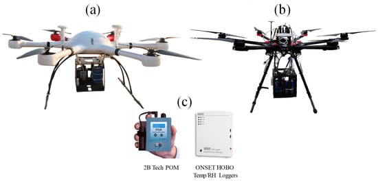
Figure 1.
Pictures of (a) the JOUAV platform, (b) DJI M600 platform, and (c) portable instruments.
Portable instruments were mounted on the UAV platforms to measure air pollutant concentrations and meteorological parameters (Figure 1c). Vertical distributions of ozone were measured by a portable ozone monitor (Model: POM, 2B Technology, USA), which is based on ultraviolet absorption. Ambient air temperature (T) and relative humidity (RH) were measured during the flights using a meteorological sensor (Model: UX12, ONSET, Australia). Specific parameters of the instruments used in this study are summarized in Table 1. As shown in Figure 1, instruments were mounted or attached inside a carbon fiber cabinet. A section of Tygon® sampling tube was linked to the inlet of POM in order to introduce the ambient sample air. This tube is FEP-lined in order to reduce the ozone loss inside the tube. The portable instruments installed on the two UAV platforms were identical. For detailed information about the UAV platform and instruments, the reader is referred to Wang et al. [21].

Table 1.
Summary of the instruments and associated parameters.used on the unmanned aerial vehicle platforms.
2.2. Description of the Experimental Site
The annual means of accumulated precipitation and surface air temperature of Shanghai is 1166.1 mm·yr−1 and 16.0 ℃, respectively [36]. The field campaigns were carried out over grassland in Feng’xian District (30°48′53″ N, 121°29′37″ E). The experimental site (Figure 2) is situated about 2 km to the southwest of the Feng’xian Campus of East China University of Science and Technology (ECUST). The experimental site is surrounded by suburban and bay area. A large chemical industry is about 2 km southwest from the site. During the study period, the average surface air temperature decreased from about 14 ℃ in November to about 7 ℃ in December. In addition, the experimental site mainly experienced sunny or cloudy weather, with a dominant wind from the north and northeast.
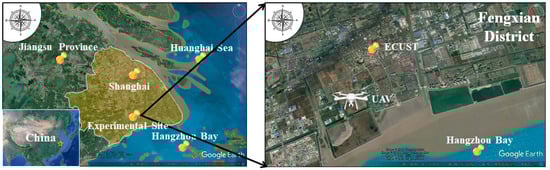
Figure 2.
Maps showing the location of the experimental site (from Google Earth).
2.3. Field Campaign
Between 26 November and 21 December 2017, 41 profiles were successful collected (Table 2). A pilot with the Aircraft Owners and Pilots Association of China (AOPA–China) certificate remotely controlled the UAV. The UAV ascended and descended with a speed of 2 m/s. This provides adequate time for the portable instruments to obtain reliable measurements. Before the UAV took off, the recording times on all the portable instruments was manually adjusted to the local time (UTC + 8) [32] in order to synchronize the measurements. The POM warmed up for at least 30 min before each flight to stabilize the measurements [18].
Table 2.
Summary of the field campaign schedule.
In this study, JOUAV was used as the primary UAV platform. From 26 November to 06 December 2017, the JOUAV malfunctioned. To continue the field experiments, the M600 platform was used as an alternative UAV platform. During the study period, joint experiments via a tethered balloon were also performed in the Feng’xian Campus of East China University of Science and Technology. Therefore, the performance of portable instruments on the UAV was compared with the tethered balloon platform. The comparison experiments were both performed on the surface and during flights. The results of the comparison has been presented in the Supplementary Materials. The specific field campaign schedule is summarized in Table 2.
2.4. Other Data Resources
A supportive meteorological dataset was obtained from the National Oceanic and Atmospheric Administration (NOAA). To study the influence of horizontal transport of air masses, the Internet-based model of hybrid single-particle Lagrangian integrated trajectory (HYSPLIT) was used to carry out backward trajectories analyses. The meteorological input for archived meteorology and HYSPLIT were both the Global Data Assimilation System meteorological dataset, with temporal resolutions of 3 h and 6 h, respectively. The sounding balloon data at 08:00 LT were obtained from the online website [37].
3. Results
3.1. UAV Platform Verification
Before using UAV platforms to perform vertical ozone observations, the uncertainties of portable monitors need to be studied first, which ensures the availability of the data. As shown in Figure S1 and Table S1, the ground-based comparison indicated that the ozone monitor on the UAV platform is in good agreement with the conventional instrument on the tethered balloon platform.
Previously in May 2016, Li et al. [38] performed comparison experiments between a fixed-wing UAV platform and the tethered balloon platform. The instruments and experimental site were identical to this study. According to three pairs of ozone profiles, although there were slight variations in ozone concentrations, the ozone measurements of the POM have also been generally consistent with the instruments used on a tethered balloon platform [38]. As for hexacopter UAV platforms, Guimarães et al. [23] used the same platform (M600) and ozone monitor (POM), and successfully obtained fifty-seven ozone profiles from March to May, 2018 in Brazil, indicating the possible use of UAV in improving atmospheric measurements of ozone. In this study, the comparison results of two pairs of ozone profiles are presented in Figure S2 and Table S1, which also indicate good consistency between the two platforms.
As shown in Figure 3, the PBL height ranged from 200–1300 m from November to December, 2017. Consequently, the UAV platforms in this study are reliable and practical to capture the vertical variations of ozone within the lower troposphere in the wintertime.
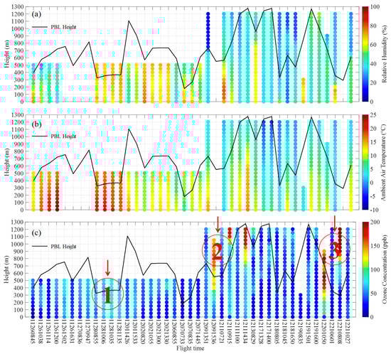
Figure 3.
Vertical profiles of (a) Relative humidity (RH), (b) ambient air temperature, and (c) ozone concentration measured by the UAV platform from 08:45 LT on 26 November to 10:27 LT on 11 December, 2017. Each label of the horizontal axis represents the profile number, which consists of the date and the exact takeoff time of each flight. The planetary boundary layer heights are shown as black solid lines. The original PBL data were obtained from the NOAA Archived Meteorology. A low-order linear interpolation method was used to calculate the estimated the PBL height during each flight period.
3.2. Overview of Vertical Profiles
3.2.1. Data Processing
After the vertical observations, data processing was performed to draw effective vertical profiles. First, ozone outliers (negative or abnormal measurements) were removed. Abnormal measurements are defined as ozone measurements that are five times higher or lower than the measurements observed during adjacent moments. Negative ozone measurements are sometimes caused by ozone concentrations near 0 ppb or low air temperature (less than 0 ℃). Considering that the outlet of the air sampling tube was placed upward, the measurements obtained during the descent were not analyzed. The updraft caused by the UAV during the descent can lead to unreliable measurements.
3.2.2. Vertical Profiles Visualization
As shown in Figure 3, 41 vertical profiles of ozone, ambient air temperature, and RH obtained during the study were visualized in a colormap. After December 9, 2017, the JOUAV platform was used. Hence, the maximum flight height extended from 500 m to 1200 m. In general, there is more detailed and complete information in the 1200–m profiles than the 500–m profiles. From 26 November to 21 December, 2017, both the average ambient air temperature and the average RH kept decreasing. This indicated a cold front passage. For the ozone profiles, the ozone concentrations aloft were generally higher than those near the surface. The ozone concentration ranged from 25–200 ppb. The maximum ozone concentration of 220 ppb was observed on the morning of December 21 over 800 m.
3.3. Vertical Characteristics of Winter Ozone
The ozone profiles observed in this study have been presented In previous sections. In this section, a systematic classification of winter ozone within the boundary layer will be given. The 41 profiles could be classified into four categories: (1) the well-mixed profile; (2) altitudinal increasing profile; (3) stratification profile; and (4) spike profile. In some flights, different categories of ozone profiles were co-existing owing to the atmospheric structure. The detailed characteristics of each profile are discussed below.
3.3.1. Well-Mixed Profile
This category of winter ozone is characterized by stagnant ozone concentrations within a certain height, with a concentration difference less than 10 ppb. An example of one dataset representative of well-mixed profiles (34%) is the profile observed at 10:27 LT on December 21 (Figure 4b). The ozone concentrations remained steady at about 35 ppb from 0–800 m. Among those profiles, the average ozone concentration was 41 ppb, which is close to the surface ozone concentration (about 5 ppb). A high average ozone concentration of 66 ppb occurred on November 26 and 28. Generally, well-mixed profiles are typical in the daytime while there is good vertical mixing, no significant horizontal transport processes, and temperature inversions. Hence, the ozone level is primarily determined by in situ production.
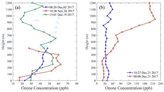
Figure 4.
Typical ozone profiles obtained by the UAV platform in the winter of 2017.
3.3.2. Altitudinal Increasing Profile
This category of winter ozone is characterized by a stable increase of ozone concentration from the surface to a certain height. An example of a dataset representative of altitudinal increasing profiles (23%) is the profile observed at 08:20 LT on December 02 (Figure 4a). The ozone concentration linearly increased from 22 ppb at the surface to 48 ppb at 500 m. Eight of the ten altitudinal profiles was observed from 07:00–10:00 LT. Generally, positive gradients are typical in ozone profiles in the morning. With weak solar radiation, the local ozone formation in the morning is slower than the depletion of ozone (i.e., NO titration, dry and wet depletion), especially in winter.
3.3.3. Stratification Profiles
This category of winter ozone is characterized by a two-layered or three-layered structure. An example of a dataset representative of stratification profiles (26%) is the profile observed at 08:08 LT on December 21 (Figure 4b). Within 400 m, the ozone concentration is about 25 ppb. Two significant interfaces were located at 400 m and 800 m. Within each interface, the ozone concentration sharply increased. Ultimately, the ozone concentration remained stable at 220 ppb over 900 m. Stratification profiles observed in this study mostly occurred in the morning. In winter, the average daily PBL height is often lower than the other seasons [39]. According to previous research, this ozone stratification is generally related to the growth of PBL or the formation of nocturnal residual layers [10].
3.3.4. Spike Profile
This category of winter ozone is characterized by extreme low and high ozone concentrations at the mid altitudes, which make profiles spike-shaped. Two examples of dataset representative of spike profiles (18%) are the profiles observed at 15:01 LT on December 19 and at 10:38 on November 26 (Figure 4a). In this study, the spike profiles were related to ozone elevation events. At 15:01 LT of December 19, 2017, an ozone elevation was observed between 200–650 m. The peak ozone concentration was as high as 60 ppb at 600 m, which was higher than the ozone concentration of 30 ppb at both the surface and at 1200 m. During this flight period, the estimated PBL height was 1269 m. Within the boundary layer, an ozone spike at mid altitudes could be attributed to the influence of the long-range transport of air masses.
In conclusion, well-mixed and altitudinal increasing profiles often occurred within short height ranges, which could be summarized as a simple structure. With the help of the JOUAV platform, more complicated ozone structures were captured from 0–1200 m. The stratification profiles and spike profiles could be recognized as a combination of simpler structures. According to Zheng et al. [15], the vertical profiles of ozone within 5 km was classified into five groups, which are highly related to meteorological parameters, thermal and dynamic factors, and regional transport. However, the vertical pattern of ozone within the boundary layer has not been fully understood. In this next section, further discussions are given to study the relationships between vertical ozone distributions and other meteorological parameters.
4. Discussion
From 27 to 28 November 2017, an ozone elevation event was observed (hollow circle 1 in Figure 3c) near the surface. The average ozone concentration at 10:00 LT on 26 November (16 ppb) was lower than that of 64 ppb at 10:35 on November 28. High surface ozone concentrations of over 60 ppb occurred in all four profiles on 28 November. After 07 December, several ozone elevations events were observed aloft. Extreme high ozone concentrations over 180 ppb were observed at 09:15 LT (182 ppb), 14:34 LT (181 ppb) on 11 December, and 08:08 LT (220 ppb) on 21 December 2017, respectively. Hence, ozone distributions at the upper air are quite different from near the surface during the study period.
4.1. Typical Ozone Elevation within 500 m
As shown in Figure 3b, significant warming was observed from the surface to 500 m from November 26 to 28, 2017. According to Table 3, with the decrease in cloud cover percentage (from 85.4% on November 26 to 5.3% on November 28), the solar radiation intensity in the morning peaked on November 28 among the three days. The photochemical reaction favors higher temperature and stronger solar radiation in clear days. Therefore, the ozone formation was enhanced during this period. Moreover, PBL height at about 10:00 of November 28 (about 350 m) was lower than two days before (400–800 m). Low PBL heights restrained the dispersion and vertical mixing of ozone. Therefore, in situ formation mainly contributes to the surface ozone elevation from November 27 to 28.
Table 3.
Meteorological data obtained from National Oceanic and Atmospheric Administration (NOAA) and sounding balloons.
Trajectories at 300 m (Figure 5a) show that the origin of air masses were the Middle-Lower Yangtze Plain. On November 28 (Figure 5b), the air masses partially came from the southeast coast of China and the Huanghai Sea. It could be distinguished by the RH profiles with average RH values of about 66% on November 28 (Figure 3a). The Middle-Lower Yangtze Plain and the southeast coast of China have been widely recognized as polluted areas. In the journey, pollutants were transported by air flows to the experimental site and contributed to the ozone elevation events.
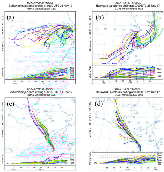
Figure 5.
The 48-h backward trajectories starting at 10:00 LT on (a) 26 November, (b) November 28 at 300 m; 48-h backward trajectories starting at (c) 09:00 LT on 11 December, and (d) 08:00 LT on December 21, 2017 at 800 m. Figures courtesy National Oceanic and Atmospheric Administration (NOAA) Air Resources Laboratory.
4.2. Ozone Elevation in the Upper Air
During the study period, several ozone elevation events were observed over 500 m. In December of 2017, the experimental site experienced a cold front passage. This is inferred by the decrease in RH and ambient air temperature in December, 2017 (Figure 3a,b). Trajectories on 11 December and 21 December (Figure 5c,d) indicate that the air masses during these days originated from the high altitudes of Outer Mongolia and then traveled straight southeast, and ultimately arrived at the experimental site.
As summarized in the last section, the ozone profile observed at 08:08 LT on December 21 (Figure 4b) and at 09:15 LT on 11 December (hollow circle 2 in Figure 3c), 2017 could be classified as stratification profiles. A significant ozone-elevated layer was located over about 800 m. However, a well-mixed ozone profile was observed about 1–2 h before each ozone-elevated profile (profile 12210601 and 12110721 in Figure 3c). Twenty-four hours earlier, the air masses traveled across the North China Plain (NCP), one of the most polluted regions in China.
The vertical trajectories (Figure 5c,d) suggest that the air masses experienced a sinking motion during the journey to Shanghai. For the RH profile on the mornings of December 11 and 21, stratification structures were observed in both. A sharp decrease in RH was observed in the upper air. The location of RH stratification is consistent with the corresponding PBL height. Seguel et al. [33] has concluded that the sharp decrease of water vapor could be an important factor to trace the downward transport of ozone from the higher troposphere or stratosphere during the passage of cold front. According to the wind data at 08:00 LT on December 11 and December 17 (Table 3), the wind directions at about 200 m or about 1000 m were all northwest or northeast. The wind speeds range from 2 to 4 m/s. Considering that the solar radiation was not strong in the morning, the ozone pollutions were possibly from the developed regions in the north. The ozone accumulated via the sinking motion and then arrived at the upper air of the experimental site. Unfortunately, the ozone data in this study could not verify this assumption, which is a point of future research.
5. Conclusions
The present study focused on the vertical observations of ozone within 1200 m in Shanghai in the winter of 2017. Using hexacopter UAV monitoring platforms equipped with portable ozone monitors, 41 vertical ozone profiles were successfully obtained within the boundary layer. The UAV observations were reliable to capture the vertical variations of winter ozone within the boundary layer. The conclusions and main contributions of this study are given as follows:
- (1)
- This study made a systematic classification of winter vertical ozone distributions. According to the 41 vertical ozone profiles obtained via the UAV platforms during the two months, the characteristics of ozone profiles were classified into four groups: well-mixed profile, altitudinal increasing profile, stratification profile, and spike profile, respectively. The number of ozone profiles in each group was evenly distributed. First, the well-mixed profiles were frequently found in the afternoon of sunny days because of good vertical mixing. Second, the altitudinal increasing profiles mainly occurred in the morning, which is related to the depletion of ozone near the ground. Third, the occurrence of stratification profiles is firmly related to the low PBL heights in the winter. Finally, extremely high or low ozone concentrations were found in the spike profiles, which may be attributed to the horizontal transport of air masses. The classification results were mostly consistent with the former research performed in the spring of the YRD region.
- (2)
- In the winter, although surface ozone level was low, ozone elevation events occurred at the upper air. The maximum ozone concentration observed from November to December, 2017 was 220 ppb. Ozone elevation events frequently occurred in the early morning, and were caused by in situ formation, horizontal, and vertical transport of air masses. First, typical in situ ozone production in the winter can be attributed to different conditions including strong radiation, high air temperature, and low PBL height. Second, typical downward flow of ozone was accompanied with a layered-structure RH profile with low RH value aloft. Third, backward trajectories also indicate that the ozone elevations were influenced by transport from the northern regions of China and from higher altitudes.
Our contributions lie in at least two aspects. First, this study provides the possibility of using hexacopter UAV platforms to perform the vertical distribution of ozone. For relevant observations in the future, researchers can use UAVs equipped with other instruments to measure vertical distributions of air pollutants such as particle matters, NOx, VOC, etc. This may help to better improve the development of vertical observation technology. Second, although the current investigation is preliminary, it provides a systematic classification of winter ozone distribution within the boundary layer. This may potentially provide valuable data support for air quality and climate models.
In the future, we will extend this study to comprehensively characterize the winter ozone by conducting more experiments at night. Furthermore, the results will be further compared with experiments performed in other seasons. These efforts, in addition to the current investigation will provide a further understanding of the roles of ozone in winter.
Supplementary Materials
The following are available online at https://www.mdpi.com/2071-1050/11/24/7026/s1. Figure S1: Ground-based comparisons of ozone concentrations: (a)Times series of ozone concentrations between the UAV platform and the tethered balloon; (b) Linear regressions between the UAV platform and the tethered balloon. The light gray dash line is the 1:1 reference line. Measurements were all averaged at 1-min intervals; Figure S2: Comparisons of vertical profiles between the UAV platform (triangles) and the tethered balloon (circles): (a) Vertical profiles captured during UAV’s ascent period (profile 1); (b) Vertical profiles captured during UAV’s descent period (profile 2) between 16:30–17:30 LT on December 18, 2017. Measurements were all averaged at 50-m intervals; Table S1: Summary of calculated metrics for ozone monitors used on the UAV platforms and the tethered balloon platform.
Author Contributions
For this article, Q.C., D.W., and X.L. conceived this study. B.L. and R.S. built the UAV platform; Q.C. analyzed the data; Q.C., H.H., and Z.P. wrote the paper.
Funding
This research was funded by the National Key R&D Program of China (grant number 2016YFC0200500); the National Planning Office of Philosophy and Social Science (grant number 16ZDA048); and the National Natural Science Foundation of China (grant number 11672176).
Acknowledgments
We would like to acknowledge the support of the Shanghai Environmental Monitoring Center and East China University of Science and Technology for the observational data of the tethered balloon platform.
Conflicts of Interest
The authors declare no conflicts of interest.
References
- Chiquetto, J.B.; Silva, M.E.S.; Cabral-Miranda, W.; Ribeiro, F.N.D.; Ibarra-Espinosa, S.A.; Ynoue, R.Y. Air quality standards and extreme ozone events in the são paulo megacity. Sustainability 2019, 11, 3725. [Google Scholar] [CrossRef]
- Geng, F.; Tie, X.; Xu, J.; Zhou, G.; Peng, L.; Gao, W.; Tang, X.; Zhao, C. Characterizations of ozone, NOx, and VOCs measured in Shanghai, China. Atmos. Environ. 2008, 42, 6873–6883. [Google Scholar] [CrossRef]
- Tang, H.; Liu, G.; Zhu, J.; Han, Y.; Kobayashi, K. Seasonal variations in surface ozone as influenced by Asian summer monsoon and biomass burning in agricultural fields of the northern Yangtze River Delta. Atmos. Res. 2013, 122, 67–76. [Google Scholar] [CrossRef]
- Wang, L.; Bai, Y.; Zhang, F.; Wang, W.; Liu, X.; Krafft, T. Spatiotemporal Patterns of Ozone and Cardiovascular and Respiratory Disease Mortalities Due to Ozone in Shenzhen. Sustainability 2017, 9, 559. [Google Scholar] [CrossRef]
- Wang, T.; Xue, L.; Brimblecombe, P.; Lam, Y.F.; Li, L.; Zhang, L. Ozone pollution in China: A review of concentrations, meteorological influences, chemical precursors, and effects. Sci. Total Environ. 2017, 575, 1582–1596. [Google Scholar] [CrossRef]
- Xu, J.; Zhu, Y.; Li, J. Seasonal Cycles of Surface Ozone and NOx in Shanghai. J. Appl. Meteorol. 1997, 36, 1424–1429. [Google Scholar] [CrossRef]
- Hernández-Paniagua, I.; Lopez-Farias, R.; Piña-Mondragón, J.; Pichardo-Corpus, J.; Delgadillo-Ruiz, O.; Flores-Torres, A.; García-Reynoso, A.; Ruiz-Suárez, L.; Mendoza, A. Increasing Weekend Effect in Ground-Level O3 in Metropolitan Areas of Mexico during 1988–2016. Sustainability 2018, 10, 3330. [Google Scholar] [CrossRef]
- Wang, L.; Wang, H.; Liu, J.; Gao, Z.; Yang, Y.; Zhang, X.; Li, Y.; Huang, M. Impacts of the near-surface urban boundary layer structure on PM2.5 concentrations in Beijing during winter. Sci. Total Environ. 2019, 669, 493–504. [Google Scholar] [CrossRef]
- Zhao, S.; Xu, Y. Exploring the Spatial Variation Characteristics and Influencing Factors of PM2.5 Pollution in China: Evidence from 289 Chinese Cities. Sustainability 2019, 11, 4751. [Google Scholar] [CrossRef]
- Klein, A.; Ravetta, F.; Thomas, J.L.; Ancellet, G.; Augustin, P.; Wilson, R.; Dieudonné, E.; Fourmentin, M.; Delbarre, H.; Pelon, J. Influence of vertical mixing and nighttime transport on surface ozone variability in the morning in Paris and the surrounding region. Atmos. Environ. 2019, 197, 92–102. [Google Scholar] [CrossRef]
- Megie, G.J.; Ancellet, G.; Pelon, J. Lidar measurements of ozone vertical profiles. Appl. Opt. 1985, 24, 3454–3463. [Google Scholar] [CrossRef] [PubMed]
- Chen, C.-L.; Tsuang, B.-J.; Tu, C.-Y.; Cheng, W.-L.; Lin, M.-D. Wintertime vertical profiles of air pollutants over a suburban area in Central Taiwan. Atmos. Environ. 2001, 36, 2049–2059. [Google Scholar] [CrossRef]
- Lin, C.-H.; Wu, Y.-L.; Lai, C.-H.; Lin, P.-H.; Lai, H.-C.; Lin, P.-L. Experimental investigation of ozone accumulation overnight during a wintertime ozone episode in south Taiwan. Atmos. Environ. 2004, 38, 4267–4278. [Google Scholar] [CrossRef]
- Zheng, X.; Chan, C.; Cui, H.; Qin, Y.; Chan, L.; Zheng, Y.; Lee, Y. Characteristics of vertical ozone distribution in the lower troposphere in the Yangtze River Delta at Lin’an in the spring of 2001. Sci. China Ser. D Earth Sci. 2005, 48, 1519–1528. [Google Scholar] [CrossRef]
- Zhang, K.; Zhou, L.; Fu, Q.; Yan, L.; Bian, Q.; Wang, D.; Xiu, G. Vertical distribution of ozone over Shanghai during late spring: A balloon-borne observation. Atmos. Environ. 2019, 208, 48–60. [Google Scholar] [CrossRef]
- Zhang, K.; Wang, D.; Bian, Q.; Duan, Y.; Zhao, M.; Fei, D.; Xiu, G.; Fu, Q. Tethered balloon-based particle number concentration, and size distribution vertical profiles within the lower troposphere of shanghai. Atmos. Environ. 2017, 154, 141–150. [Google Scholar] [CrossRef]
- Zhang, K.; Zhou, L.; Fu, Q.; Yan, L.; Morawska, L.; Jayaratne, R.; Xiu, G. Sources and vertical distribution of PM2.5 over Shanghai during the winter of 2017. Sci. Total Environ. 2019. [Google Scholar] [CrossRef]
- Li, X.-B.; Wang, D.-S.; Lu, Q.-C.; Peng, Z.-R.; Lu, S.-J.; Li, B.; Li, C. Three-dimensional investigation of ozone pollution in the lower troposphere using an unmanned aerial vehicle platform. Environ. Pollut. 2017, 224, 107–116. [Google Scholar] [CrossRef]
- Li, X.-B.; Wang, D.; Lu, Q.-C.; Peng, Z.-R.; Fu, Q.; Hu, X.-M.; Huo, J.; Xiu, G.; Li, B.; Li, C.; et al. Three-dimensional analysis of ozone and PM2.5 distributions obtained by observations of tethered balloon and unmanned aerial vehicle in Shanghai, China. Stoch. Environ. Res. Risk Assess. 2018, 32, 1189–1203. [Google Scholar] [CrossRef]
- Peng, Z.-R.; Wang, D.; Wang, Z.; Gao, Y.; Lu, S. A study of vertical distribution patterns of PM2.5 concentrations based on ambient monitoring with unmanned aerial vehicles: A case in Hangzhou, China. Atmos. Environ. 2015, 123, 357–369. [Google Scholar] [CrossRef]
- Wang, D.; Wang, Z.; Peng, Z.R.; Wang, D. Using unmanned aerial vehicle to investigate the vertical distribution of fine particulate matter. Int. J. Environ. Sci. Technol. 2019. [Google Scholar] [CrossRef]
- Watai, T.; Machida, T.; Ishizaki, N.; Inoue, G. A lightweight observation system for atmospheric carbon dioxide concentration using a small unmanned aerial vehicle. J. Atmos. Ocean. Technol. 2006, 23, 700–710. [Google Scholar] [CrossRef]
- Guimarães, P.; Ye, J.; Batista, C.; Barbosa, R.; Ribeiro, I.; Medeiros, A.; Souza, R.; Martin, S.T. Vertical Profiles of Ozone Concentration Collected by an Unmanned Aerial Vehicle and the Mixing of the Nighttime Boundary Layer over an Amazonian Urban Area. Atmosphere 2019, 10, 599. [Google Scholar] [CrossRef]
- Visconti, G. Airborne measurements and climatic change science: Aircraft, balloons and UAV, s. Mere SA It 2008, 79, 849–852. [Google Scholar]
- Aneja, V.P.; Mathur, R.; Arya, S.P.; Li, Y.; Murray, G.C.; Manuszak, T.L. Coupling the vertical distribution of ozone in the atmosphere boundary layer. Environ. Sci. Technol. 2000, 34, 2324–2329. [Google Scholar] [CrossRef]
- Tang, H.; Liu, G.; Zhu, J.; Han, Y.; Kobayashi, K. Seasonal variations in surface ozone and its precursors over an urban site in India. Atmos. Res. 2013, 36, 1424–1429. [Google Scholar]
- Varotsos, C. Solar ultraviolet radiation and total ozone, as derived from satellite and ground-based instrumentation. Geophys. Res. Lett. 1994, 21, 1787–1790. [Google Scholar] [CrossRef]
- Zhao, H.; Zheng, Y.; Li, C. Spatiotemporal Distribution of PM2.5 and O3 and Their Interaction during the Summer and Winter Seasons in Beijing, China. Sustainability 2018, 10, 4519. [Google Scholar] [CrossRef]
- Brown, S.S.; Dubé, W.P.; Osthoff, H.D.; Wolfe, D.E.; Angevine, W.M. High resolution vertical distributions of NO3 and N2O5 through the nocturnal boundary layer. Atmos. Chem. Phys. Discuss. 2007, 7, 139–149. [Google Scholar] [CrossRef]
- Jenkin, M.E.; Clemitshaw, K.C. Ozone and other secondary photochemical pollutants: Chemical processes governing their formation in the planetary boundary layer. Atmos. Environ. 2000, 34, 2499–2527. [Google Scholar] [CrossRef]
- Lyman, S.; Tran, T. Inversion structure and winter ozone distribution in the Uintah Basin, Utah, U.S.A. Atmos. Environ. 2015, 123, 156–165. [Google Scholar] [CrossRef]
- Rappenglück, B.; Ackermann, L.; Alvarez, S.; Golovko, J.; Buhr, M.; Field, R.; Soltis, J.; Montague, D.C.; Hauze, B.; Adamson, S.; et al. Strong wintertime ozone events in the Upper Green River Basin, Wyoming. Atmos. Chem. Phys. Discuss. 2013, 13, 17953–18005. [Google Scholar] [CrossRef]
- Seguel, R.J.; Mancilla, C.A.; Leiva, G.M.A. Stratospheric ozone intrusions during the passage of cold fronts over Central Chile. Air Qual. Atmos. Health 2018, 11, 535–548. [Google Scholar] [CrossRef]
- Bharti, K.; Rajat, A.; Vinay, S. Literature review and proposed conceptual framework. Int. J. Mark. Res. 2015, 57, 571–604. [Google Scholar] [CrossRef]
- Centobelli, P.; Cerchione, R.; Esposito, E. Exploration and exploitation in the development of more entrepreneurial universities: A twisting learning path model of ambidexterity. Technol. Forecast. Soc. Chang. 2019, 141, 172–194. [Google Scholar] [CrossRef]
- Shanghai Municipal Statistics Bureau (SMSB). Shanghai Statistical Yearbook; China Statistical Press: Shanghai, China, 2017.
- Atmospheric Soundings. Available online: http://weather.uwyo.edu/upperair/sounding.html (accessed on 7 December 2019).
- Li, X.-B.; Peng, Z.-R.; Lu, Q.-C.; Wang, D.; Hu, X.-M.; Wang, D.; Li, B.; Fu, Q.; Xiu, G.; He, H. Evaluation of unmanned aerial system in measuring lower tropospheric ozone and fine aerosol particles using portable monitors. Atmos. Environ. 2019. [Google Scholar] [CrossRef]
- Fan, S.; Gao, Z.; Kalogiros, J.; Li, Y.; Yin, J.; Li, X. Estimate of boundary-layer depth in Nanjing city using aerosol lidar data during 2016–2017 winter. Atmos. Environ. 2019, 205, 67–77. [Google Scholar] [CrossRef]
© 2019 by the authors. Licensee MDPI, Basel, Switzerland. This article is an open access article distributed under the terms and conditions of the Creative Commons Attribution (CC BY) license (http://creativecommons.org/licenses/by/4.0/).