Abstract
In railroad construction—in particular, direct-fixation tracks—a longitudinal concrete block known as a “plinth” is used to elevate the profiles of the railroad track from the aerial guideway (e.g., bridge deck). A post-construction alignment revision is often required if the plinth elevation surpasses its maximum tolerance after the concrete pour. In such cases, the plinth surface needs to be grinded to meet the design elevation, or a shim should be inserted underneath the rail pad to raise the profile elevation. Considering both sides of the rail plinths, vertical design factors, and performance specifications, re-optimization of the vertical profile is of great interest, but the process poses challenges and represents a practical research problem. An optimization model aimed at minimizing the cost of post-construction alignment repairs is proposed and a real-case numerical example is analyzed to check the effectiveness of the model.
1. Introduction
Alignment design plays a critical role in the construction and serviceability of horizontal transportation infrastructure. Alignment design is generally considered a control reference for interdisciplinary coordination among various design disciplines for the project. Because the alignment design of transportation infrastructure takes into account both the horizontal alignment and vertical profile, the state of practice has been to design the horizontal alignment first, and to design the vertical profiles as sub-solutions. Since such a two-step design process may not explore all possible alternatives, many studies propose techniques to optimize the three-dimensional alignment of horizontal infrastructures such as highways and railways. Jong and Schonfeld [1] proposed a genetic algorithm to optimize highway alignment based on column generation from the combinatorial optimization methods. Jha [2] expanded upon the Jong and Schonfeld [1] highway alignment optimization model by considering the spatial analysis environment, in order to develop a geographic information system-based highway optimization model. Several studies specifically explored railway alignment optimization in mountainous terrain [3,4,5]. Lai and Schonfeld [6] jointly optimized the alignment of rail transit and its station locations, given that the location of a station can effect demand distributions and spacing between stations can affect travel times. Kim et al. [7] developed an improved genetic algorithm to optimize the horizontal alignment design problem to include geographical constraints such as bridges and tunnels. Kim et al. [8] also suggested a stepwise genetic algorithm to improve the efficiency of the solution method. Many studies have explored ways to optimize both the horizontal and vertical alignments simultaneously [9,10,11].
Because vertical profiles closely relate to travel times and energy consumption, Kim and Schonfeld [12] explored vertical alignment design parameters and vehicle dynamics to minimize the cost of operations. Kim et al. [13] further applied a simulation-based optimization model to jointly optimize the vertical alignment and cruising speed. They considered a vertical alignment design known as the “dipped vertical alignment (DVA) profile” and optimized the design parameter to minimize system costs, including the cost of operators and users. Kim et al. [14] explored further to incorporate the concept of regenerative braking, recognizing that it can reduce operation costs significantly. They also considered various types of vertical alignment design. Kim et al. [15] extended their previous model to take into account the cost of construction. In that study, they considered the arc length of the vertical alignment profile to estimate the cost of construction of the rail line. Although many studies have proposed to optimize highway and railway alignments, most proposed models are limited to the planning studies.
In railroad construction projects, two types of tracks are predominantly used for general construction. One method of construction uses a ballasted track, while the other method is known as direct-fixation track construction. Ballasted track construction is typically used for at-grade construction where it is easy to maintain the track and it is cost-effective compared with other methods. For both the aerial (elevated) track and the underground track, direct-fixation track is commonly used. In direct-fixation track construction, the design elevation of the railroad profile is governed significantly by the elevation of the plinth, which is the longitudinal concrete block located below the rail. When the plinth construction is complete, the direct-fixation fastener is mounted to the plinth to anchor the rail. Because plinth construction is generally done in the field, the elevation of the plinth is subject to the quality control of the construction methods and overall workmanship. When the elevation of the plinth does not match the desirable design elevation, it offsets the rail elevation.
It is noted that post-construction alignment may yield some offset from the design alignment as construction processes can introduce some errors. Nevertheless, post-construction alignment is very important because the operation agency or project client will not accept the project if the post-construction alignment shows offsets from the design alignment. If the as-built track elevation does not match the design profile, repairs to adjust the as-built track elevation are required; this is generally done by adding shim under the rail to increase the elevation, or by grinding the plinth top surface to lower the elevation. Either way, modifications require a significant amount of resources and materials, and can lead to construction delays. We believe that revising post-construction alignment is a complex yet practical problem; however, no study has been proposed yet to address this repair challenge. To minimize repair work, this paper proposes a method to revise the vertical design profiles. The following section provides the design criteria for both the horizontal and vertical curves, followed by the repair cost formulation, numerical analysis, and conclusion.
2. Review of Design Criteria
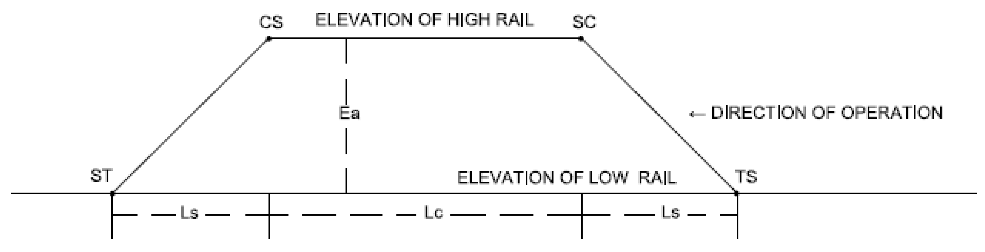
In this section, we review design criteria for horizontal and vertical curves for railway constructions. As an alignment enters a curve section, an amount of superelevation is required to prevent the train from overturning due to the centrifugal force. In Figure 1, the effect of superelevation along a horizontal curve is described as a schematic.
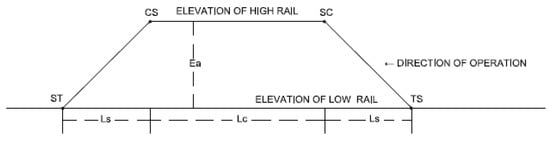
Figure 1.
Superelevation around a horizontal curve (source: authors).
As we assume the direction of travel is from right to left, the elevation of both rails is the same until the alignment enters the curve, as denoted as the tangent to spiral (TS) point. For the length of spiral curve Ls, the amount of superelevation Ea is linearly distributed between the TS and Spiral to Curve (SC) point. Between the SC and curve to spiral (CS) points, the design amount of superelevation is fully achieved and is maintained constantly. In the exit spiral, the amount of superelevation is reduced linearly within the length of the spiral.
The amount of superelevation is determined by the relation between the train speed () and the radius of the simple curve (). The Washington Metropolitan Area Transit Authority’s (WMATA) [16] design criteria for the horizontal curve design is referenced as follows. The total amount of superelevation along the curve is the sum of actual superelevation and unbalanced superelevation as shown in Equation (1).
Equation (1) is then expressed as a function of design speed () and the radius of the horizontal curve .
It is noted that the maximum amount of actual superelevation is typically four inches for at-grade construction and six inches for elevated structures [16].
In general, a horizontal railroad curve consists of a circular curve and two spiral curves, one entering and one exiting. Before the TS point, the track is tangent and the elevations of both rails are the same. When the track enters a curved alignment, the amount of superelevation, defined as , is imposed along the length of the spiral curve, . In general, the amount of superelevation is uniformly distributed in the length of spiral curve which is determined as the following:
where, is the amount of unbalanced superelevation (=).
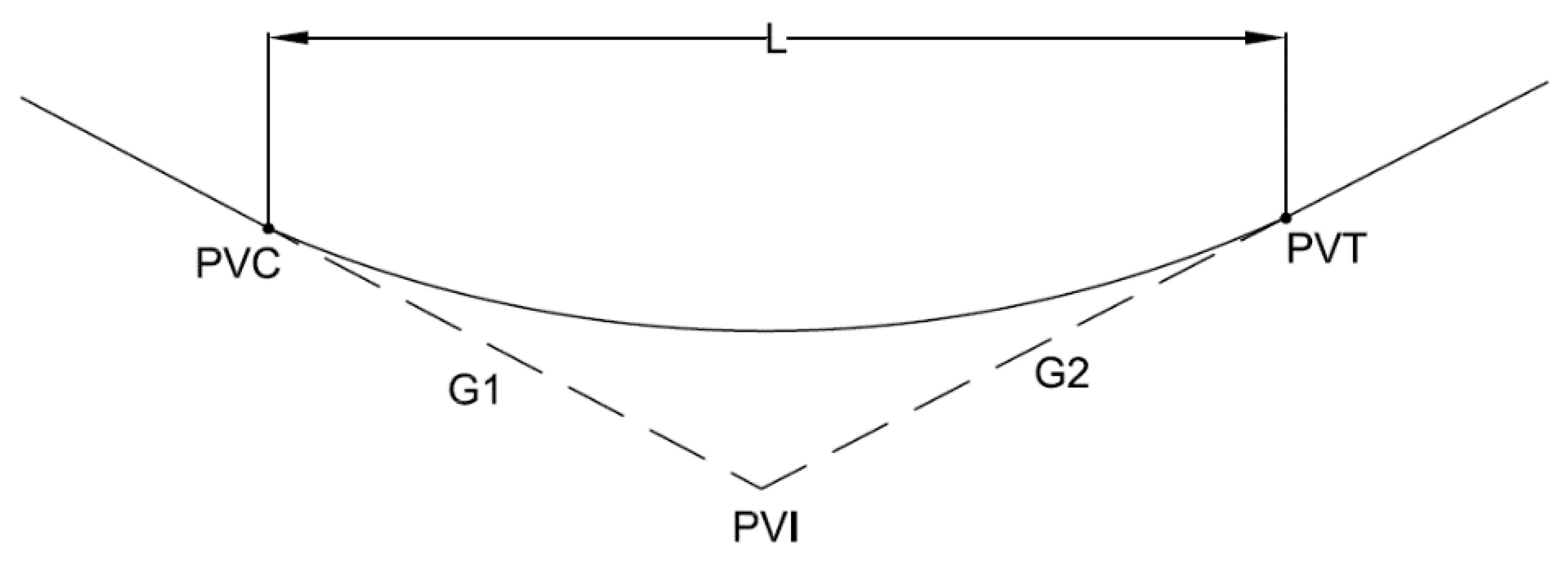
Vertical curve designs are based on a parabolic function. The parabolic formula that is used for vertical railway alignment design is as follows [17].
In Equation (7), the elevation of point of vertical curve (PVC) is used as the intercept. The entering grade () and the exit grade ( are used as a percent value. The is defined as the length of the vertical curve in stations (i.e., 100 ft). The distance away from the PVC is defined as in stations in Equation (7). Figure 2 graphically describes the relationships between variables [17].
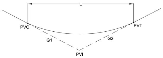
Figure 2.
Parabolic vertical curve.
If the track alignment is a tangent section, the elevations of both the left rail and the right rail are the same because the amount of superelevation is zero. When the track alignment reaches a curved segment, the low rail elevation is designated as the design elevation, and the high rail elevation is the sum of superelevation and the elevation of the low rail. The elevation of the high rail may be formulated as following:
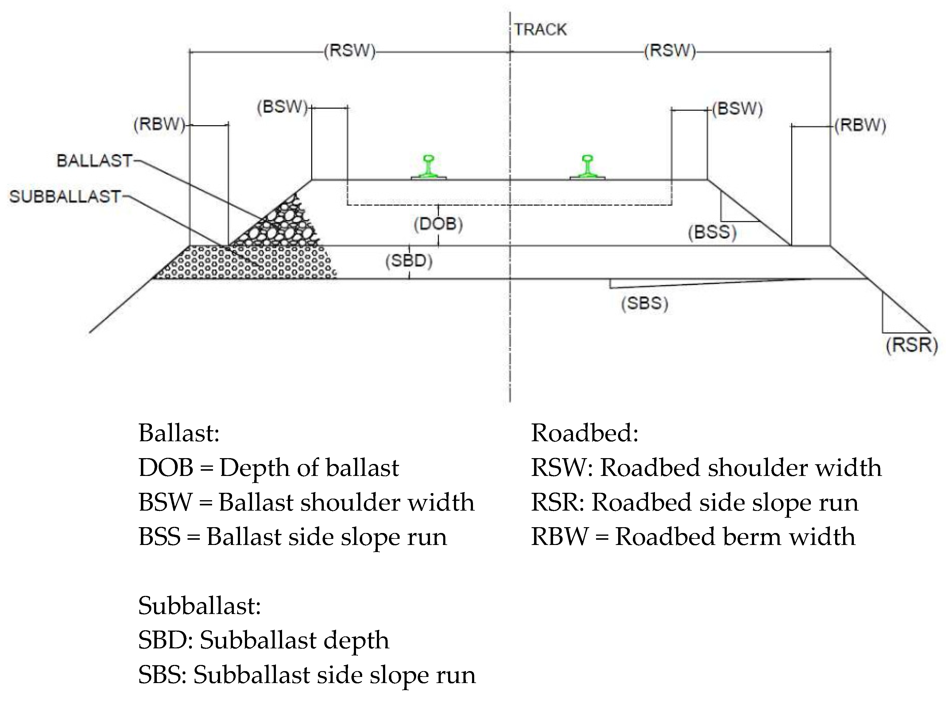
In general track construction, a ballasted track is typically used. The thickness of the ballast directly under the rail is 12 inches, and the thickness of sub-ballast is 8 inches, minimum. The typical cross-section is shown in Figure 3. The crosstie is equally spaced at 24 inches for the tangent track and is adjusted for the curved track. The ballasted track is economical and it is easy to maintain; as such, this type of track is commonly used in at-grade construction of railways.
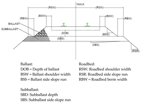
Figure 3.
Typical ballasted track [18].
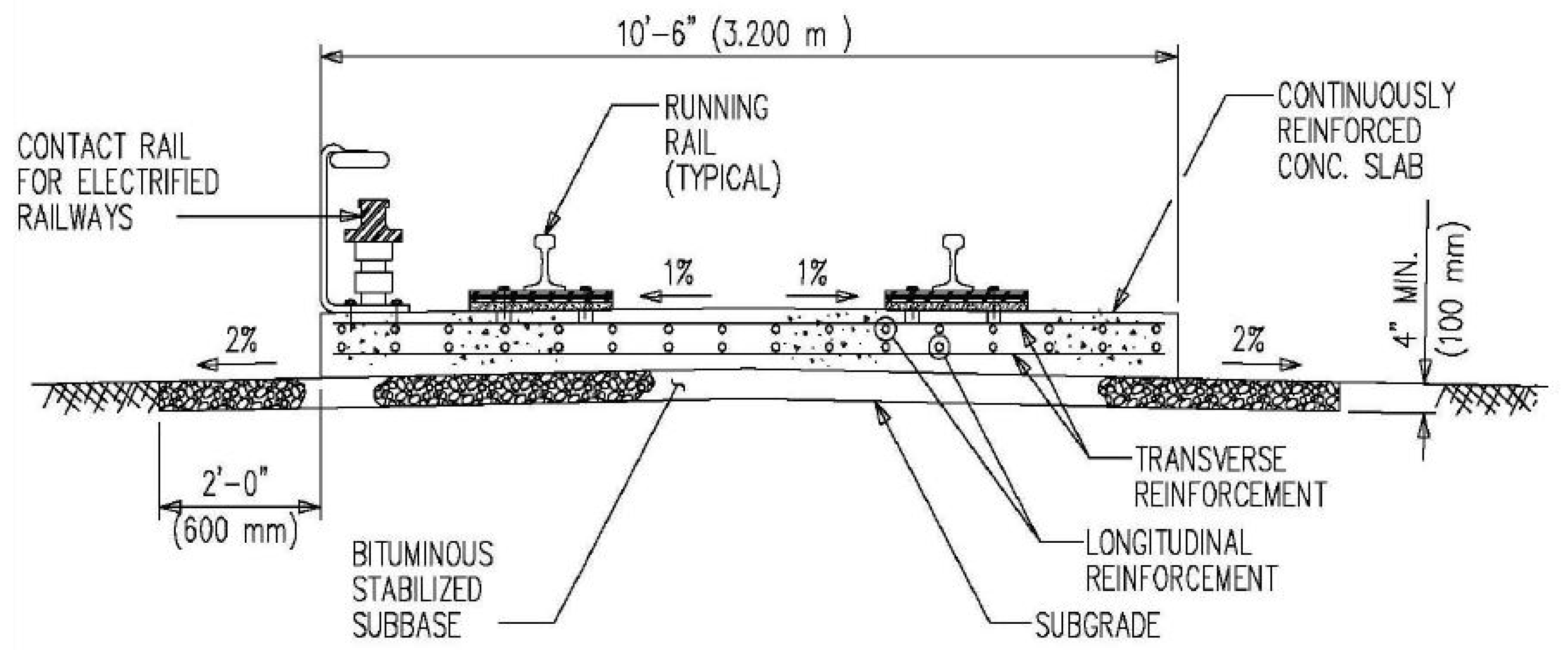
Whether the track is underground or above ground (i.e., aerial guideway), direct-fixation track construction—also referred to as a concrete slab track system (see Figure 4)—is typically used, rather than ballasted track construction. As shown in Figure 4, at the project site, reinforced concrete block is typically constructed extending longitudinally alongside the track.
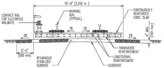
Figure 4.
Continuously reinforced typical concrete slab track system [18].
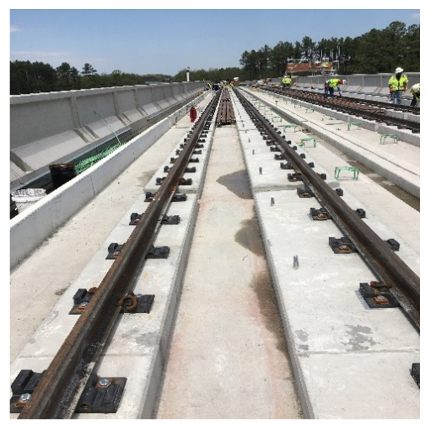
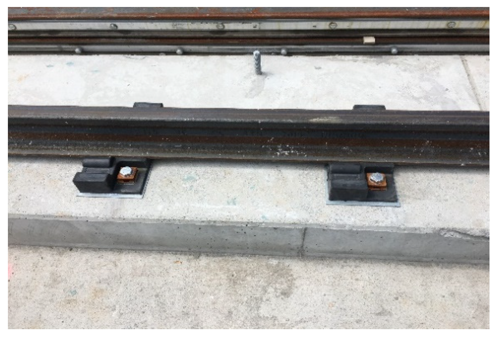
As shown in Figure 5, in direct-fixation track construction, the surface of the plinth block should be smooth and flat, while the direct-fixation fastener (DFF) system should be installed 30 inches apart longitudinally on the top surface of the plinth in order to anchor the rail. If the elevation of the plinth surpasses the construction tolerance, a repair is required either by grinding the plinth surface to lower the elevation, or by adding shim underneath the direct-fixation fastener system to raise the elevation of the rail. Figure 6 presents an example of lower plinth elevation whereby a shim is added between DFF and the plinth.

Figure 5.
Example of a direct-fixation railroad track (source: authors).

Figure 6.
Adding shim underneath direct-fixation fastener (DFF) (source: authors).
In Figure 5, it is noted that a railroad track requires two plinths, in which each plinth is constructed in a separate manner but the elevations of two plinths should be coordinated to meet the elevation of the railroad track. Because the final elevation of the rail is largely controlled by the elevation of the plinth, quality control of plinth construction is very important and repair work is generally necessary. In the next section, we present a numerical study as well as a solution method.
3. Minimum Cost Repair Model for Post-Construction Alignment
3.1. Modelling Assumptions
In this paper, we make a few assumptions in order to make the developed model practically applicable. The assumptions are as follows:
- (1)
- Construction proceeds in phase. Railway alignment includes a series of tangent and curved sections. Each section is constructed as one phase.
- (2)
- The next phase of construction does not start until the prior necessary post-construction repair work is completed.
- (3)
- The post-construction alignment revision does not affect the work provided by other disciplines. Otherwise, the necessary design revisions for other disciplines are assumed to be negligible or are revised accordingly.
3.2. Decision Variable and Constraint
In this repair model, we define the revised location of point of vertical intersection (PVI) as the decision variable. We seek the minimum repair cost by revising the alignment profile, mainly by relocating the point of vertical intersection (PVI). Specifically, we look for the horizontal stationing information for the PVI, as the vertical elevation of the PVI is assumed to be determined based on the entering slope . The exit slope is then automatically determined between the revised PVI and the PVI of the next vertical curve. When it comes to revising the PVI, we have an unlimited number of alternatives; as such, the problem has a large search space.
It is reasonable to assume that the revised PVI location may not be very far from the original design values. Thus, we incorporate a constraint for the lower and upper boundaries of the PVI station. We assumed that the new station of the PVI is in between +/−15% of the length of the initial vertical curve from the original location of the PVI. With the new location of the PVI, the exit slope is newly calculated based on the revised PVI coordinates and the next PVI coordinates.
3.3. Objective Function
The objective of the model is to minimize the cost of repair for post-construction alignment. There are two kinds of repair measures. The first involves grinding the plinth surface to lower the elevation—which requires high repair costs—and the second involves inserting a shim(s) beneath the direct-fixation fastener to raise the rail elevation. The total cost of repair is provided in Equation (9).
In Equation (9), the value of is denoted for each rail. For instance, = 1 for the low rail and = 2 for the high rail portion(s) of the alignment. The parameter is denoted as elevation checkpoints. Thus, is defined as the elevation of rail at checkpoint . The superscript a means the actual elevation and means the revised elevation. We consider a binary variable to distinguish whether grinding work is required, or shims must be installed, based on the difference between the revised profile elevation and post-construction elevation. is the unit cost of repair for grinding the plinth surface by 1/16 inch. is the unit cost of repair for inserting a shim with 1/16 inch thickness. is the conversion factor for the amount of work from ft to 1/16 inch (= 12×16).
It is noted that the elevation of the high rail is dependent on the elevation of the low rail. If the railroad track runs tangentially, the elevation of the low rail and the elevation of the high rail are the same. If the alignment is in a horizontal curve section—meaning that the superelevation is non-zero—then the elevation of the high rail is the sum of the amount of superelevation and the elevation of the low rail. Thus, by controlling the low rail elevation, the high rail is revised accordingly.
3.4. Solution Method
It is noted that the construction of the low rail plinth and the high rail plinth are managed independently, despite the fact that their rail elevations should be coordinated by the amount of superelevation along the alignment. If the repair work is required within a curved track, the re-alignment of the design can become more complicated. In such a case, the realignment of the railroad track is related to multiple design parameters in both horizontal and vertical curves. We note that there are potentially numerous alternative solutions so we employ an artificial intelligent technique (i.e., genetic algorithm as an evolutionary approach) to find the best possible solution for the minimum repair cost.
Genetic algorithms are search algorithms based on the mechanics of natural selection and natural genetics. They combine survival of the fittest among string structures with a structured yet randomized flair of human search. In every generation, a new set of artificial creatures (strings) is created using bits and pieces of the fittest of the old; an occasional new part is tried for good measure. Genetic algorithms repeatedly modify a population of individual solutions. At each step, the genetic algorithm selects individuals at random from the current population to be parents and uses them to produce the children for the next generation. Over successive generations, the population “evolves” toward an optimal solution. The genetic algorithm uses three main types of rules at each step to create the next generation from the current population: (1) selection rules select the individuals, called parents, that contribute to the population at the next generation; (2) crossover rules combine two parents to form children for the next generation; (3) mutation rules apply random changes to individual parents to form children [19].
Genetic algorithms are theoretically and empirically proven to provide robust searches in a complex space [20]. Genetic algorithms are first used to solve an optimization problem by De-Jong [21] and are used in many design studies such as alignment optimizations [8,9,15] and the scheduling of interdependent projects [22]. Specifically, how the variables are coded plays a clear role in whether or not a genetic algorithm is efficient. Real coded genetic algorithms use real numbers for encoding and offer faster convergences rather than traditional binary or gray coded genetic algorithms [23,24]; thus, we employed a real-coded genetic algorithm. Further details regarding a real coded genetic algorithm are referenced [23,25].
4. Numerical Analysis
4.1. Input Values
In this section, we generate a numerical case study using WMATA design criteria [16]. Table 1 provides the initial design parameters.

Table 1.
Input values for a case study.
In Table 2, the track is assumed to be tangent vertically and horizontally before Sta 0 + 00.00, and enters a vertical curve. We note that the length of the vertical curve is 200 ft as we see that the distance from the PVC (point of vertical curve) to the PVT (point of vertical tangent) is 200 ft. The track enters the horizontal curve at the Sta 0 + 84.86. The six inches of superelevation should be uniformly distributed along the length of 357.17 ft. At the spiral to curve (SC) point, six inches of superelevation is achieved and it is constantly maintained along the simple curve between SC and CS, which is 709.42 ft long.
Table 2.
Horizontal and vertical curve data.
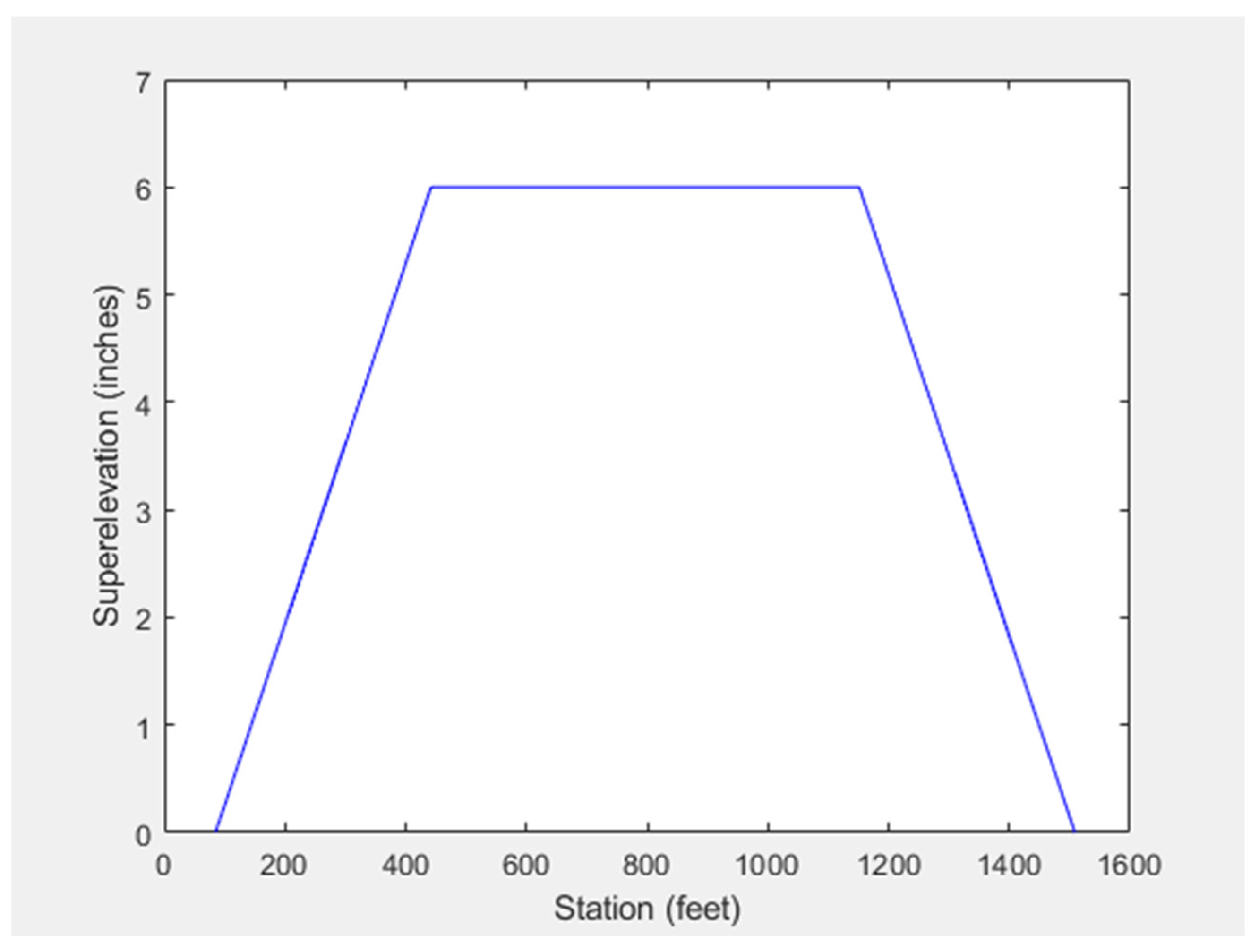
Figure 7 shows six inches of superelevation enforced between Sta 4 + 42.03 (SC) and Sta. 11 + 51.45 (CS), a circular curve, in a horizontal curve.
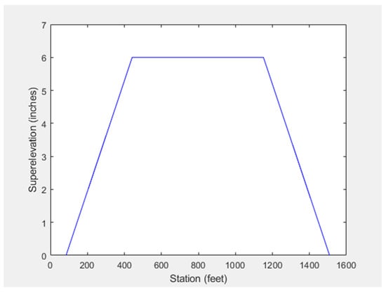
Figure 7.
Superelevation distribution for a horizontal curve (source: authors).
As Table 2 shows, a vertical curve with a length of 200 ft is considered; the vertical curve starts at Sta 0 + 00.00 and ends at Sta 2 + 00.00. The parabolic curve equation, which is based on Equation (7), is presented as follows:
where is in station (100 ft).
4.2. Estimating Vertical Profile Elevations
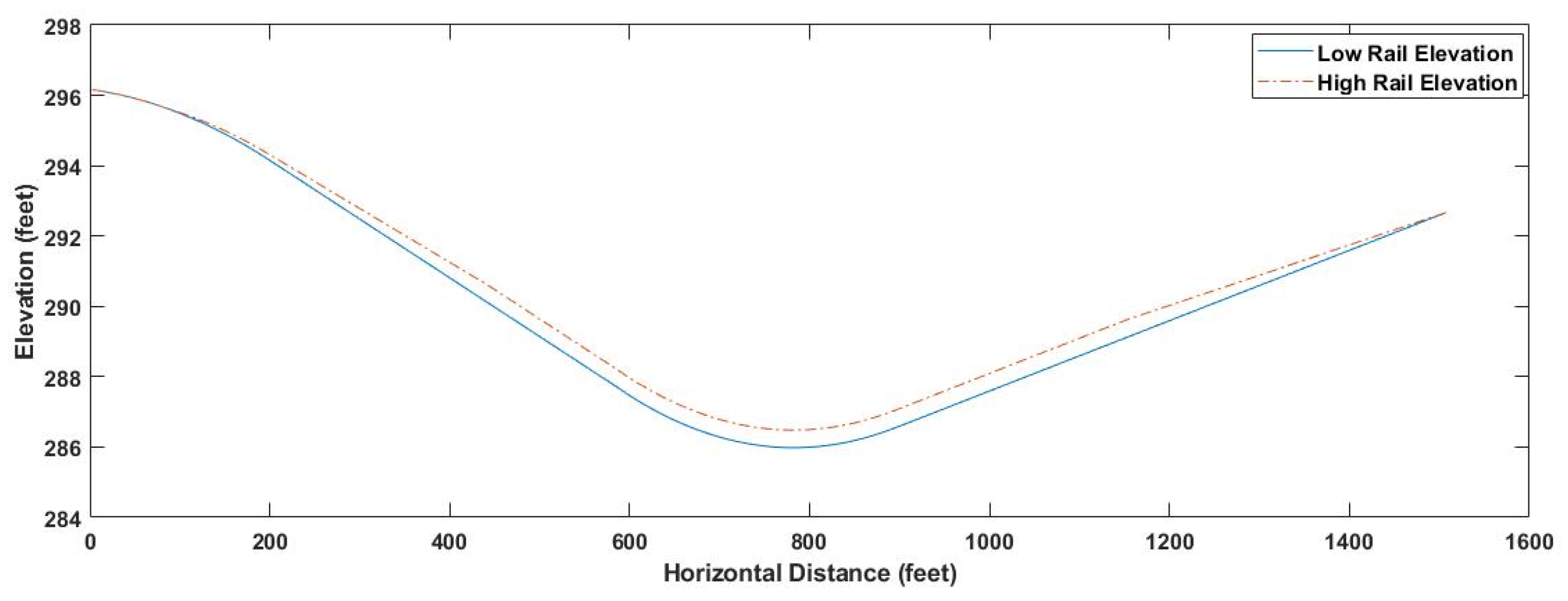
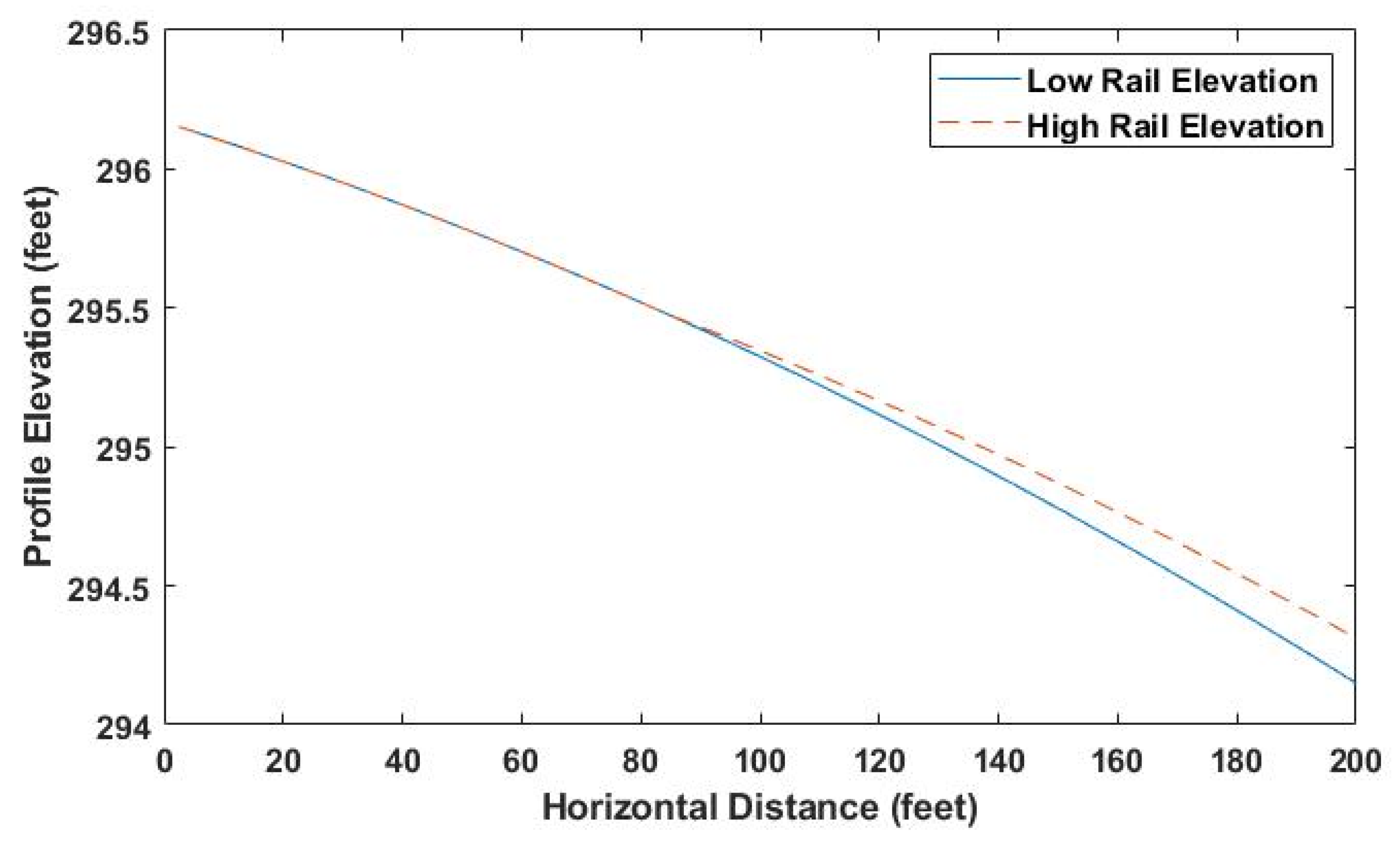
In the railroads, the design elevation always refers to the low rail elevation, as shown in Equation (10). We note that at the beginning of the vertical curve, the elevations of both rails are the same; this means that the alignment is a horizontally tangent track. The horizontal curve is introduced so that the amount of superelevation is gradually imposed, starting from Sta 0 + 84.86. The design high rail elevation is the sum of the design low rail elevation and the amount of superelevation. Figure 8 shows the vertical profiles with two curves, and Figure 9 presents the elevation of both sides of the rails in the problem area.
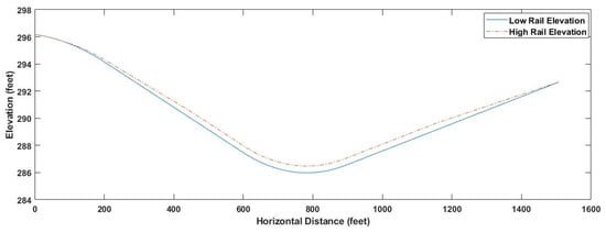
Figure 8.
Elevations of a low- and high-rail along a horizontal curve (source: authors).
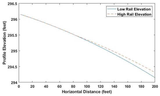
Figure 9.
Design elevation (low and high rails) along a vertical curve.
The post-construction alignment profiles are generated to verify that the post-construction alignment meets the original design alignments. However, as we discussed in the introduction, the post-construction alignment usually yields elevation offsets due to various factors (e.g., construction quality control) requiring repair work. Table 3 shows that the post-construction alignment profiles are generated in roughly 10-ft intervals.
Table 3.
Post-construction elevations in a vertical curve section.
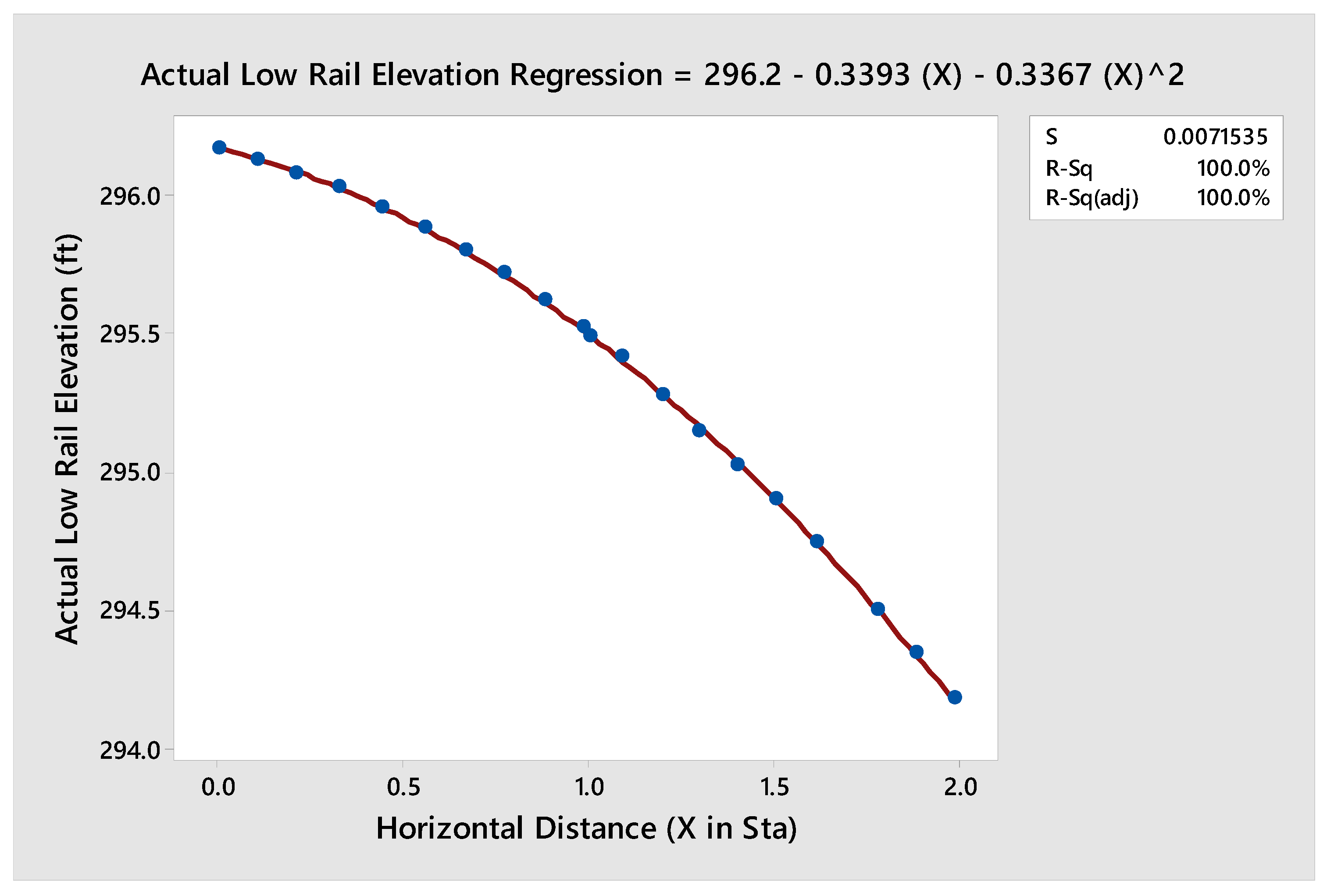
It is noted that it is not feasible to observe the elevation of post-construction at every check point. Thus, we generate regression equations that work best with the data obtained from the field. As the parabolic vertical curve formula is a second order quadratic function, we use a second order quadratic function to estimate the elevation of the low rail, as shown in Figure 10.
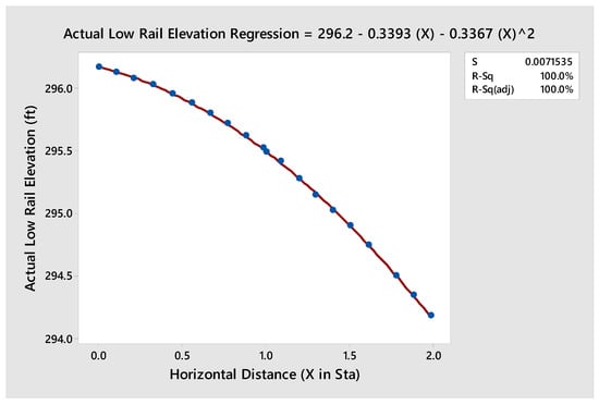
Figure 10.
Regression model for post-construction elevation of low rail in a vertical curve.
Figure 11 presents the elevation of the high side of the rail. The R2 value of 0.9921 is slightly less than the value for the estimation function shown in Figure 10. This is because the high rail elevation consists of three different sections—specifically, two spiral sections and one simple curve section. Still, we treat these three sections as one whole grouping for the regression, as the R2 value is close to 1.0.

Figure 11.
Regression model for post-construction elevation of high rail in a vertical curve.
4.3. Optimzied Design for Post-Construction Alignment
Below shows the optimal revision of the vertical curve that minimizes the cost of repair for post-construction alignments. The optimized PVI location is determined as Sta 0 + 88.29 using a genetic algorithm and corresponding elevation is found to be 295.86 ft. The resulting entering and exiting grades are −0.35% and −1.496%, respectively. Table 4 presents the repair cost breakdown as well as the initial repair cost estimates.
Table 4.
Optimized repair costs.
As shown in Table 4, the point of vertical intersection (PVI) location is relocated to minimize the cost of repair after the plinth construction. The total amount of shimming based on the revised vertical curve is 3.301 ft, and the total amount of grinding from the revised profile is 3.149 ft. The total cost of repair with optimized vertical alignment is approximately $11,866, which is $348 less than the original repair cost—equivalent to a 2.85% reduction in repair cost.
4.4. Sensitivity Analysis
In this section, we analyze the sensitivity of the repair cost with respect to the cost parameters for shimming and grinding as each project site may have different conditions for grinding repair and shimming repair. As shown in Table 5, Case 6 is used as the Baseline Case. It is noted that Cases 1, 6, 11, and 16 have the same unit costs for both shimming and grinding. Therefore, the revised PVI location is identical; it reflects the total repair cost based on the cost parameters. Cases 2 and 8 show similar results (i.e., identical PVI location) as the grinding cost is twice as high as the cost of shimming.
Table 5.
Summary of sensitivity analyses.
When the unit cost of shimming is held at $10, cases 5 through 8 provide the cost variations based on the unit cost of grinding. When the grinding unit cost is $5—which is half of the Baseline Case (Case 6)—we find that the total repair cost is reduced by 31.77%. As the unit cost of grinding is increased from $10 to $15 (from Case 6 to Case 7), the total repair cost is increased by 23.6% compared with the Baseline Case. When the unit grinding cost is twice as high as the Baseline Case (Case 8), the total repair cost is $17.264.66, which represents a 45.5% increase in the total repair cost.
Overall, it is found that, based on the input values we used for the numerical study when the grinding cost is higher, the location of the PVI increases. In other words, when the shimming unit cost is relatively higher than the cost of grinding, the location of the PVI decreases. For instance, when the shimming cost is $15 or $20, the revised PVI locations show Sta. 0 + 85, which is the lower boundary of the constraint for the new location of the PVI.
5. Conclusions
In direct-fixation track construction, the concrete plinth elevation is very important as it directly correlates with the elevation of the top of the rails. When the plinth elevation deviates from the design elevations, the concrete plinths require either surface grinding or additional shim beneath the rail fastener system. As either repair method can prove very costly, this paper proposes a method to re-optimize alignment design parameters—such as the point of vertical intersection (PVI)—to minimize the cost of repair. Because the two plinth elevations should be treated as independent blocks of concrete—despite the fact that their surfaces should be coordinated to maintain the elevation of railroad tracks, which requires the distribution of superelevation along the high rail (in the curved segment)—we consider this problem to be an optimization problem with large search regions. Thus, a genetic algorithm is selected to redesign the parameter (stationing) of the PVI location.
We consider a vertical curve section as a numerical example in order to take full consideration of the effect of superelevation from the horizontal design, and its correlations with the vertical curve design parameters. The optimized PVI is found at Sta 0 + 88.29 (it was originally at Sta 1 + 00.00) and the corresponding elevation of the revised PVI is 295.86 ft; this represents a 0.04 ft increase from the original design elevation. We find that the repair cost from the optimal revision of the post-construction alignment is reduced by 2.85% compared with the repair cost estimate based on the original alignment. A series of sensitivity analyses is presented to understand how the optimal location of the PVI and the repair cost are determined with respect to the grinding and shimming unit costs.
This research may be further extended to investigate the repair model for ballasted track in order to comprehensively cover railroad alignment repair models. This study can be easily adopted to minimize the repair cost of horizontal transportation infrastructure projects.
Author Contributions
Conceptualization and methodology: M.E.K. and E.K.; modeling and analysis: G.D., T.C. and M.E.K.; writing: M.E.K., G.D., T.C. and E.K.; supervision, M.E.K.; project administration, E.K. and M.E.K.; funding acquisition: E.K.
Funding
This research was supported by Incheon National University (International Cooperative) Research Grant in 2016.
Acknowledgments
The authors appreciate comments from four reviewers which improved the paper.
Conflicts of Interest
The authors declare no conflicts of interest.
References
- Jong, J.-C.; Schonfeld, P. An Evolutionary Model for Simultaneously Optimizing Three-Dimensional Highway Alignments. Transp. Res. Part B 2003, 37, 107–128. [Google Scholar] [CrossRef]
- Jha, M.K. A Geographic Information System-Based Model for Highway Design Optimization. Ph.D. Thesis, University of Maryland, College Park, MD, USA, 2000. [Google Scholar]
- Li, W.; Pu, H.; Schonfeld, P.; Zhang, H.; Zheng, X. Methodology for optimizing constrained 3-dimensional railway alignments in mountainous terrain. Transp. Res. Part C 2016, 68, 549–656. [Google Scholar] [CrossRef]
- Pu, H.; Zhang, H.; Li, W.; Xiong, J.; Hu, J.; Wang, J. Concurrent optimization of mountain railway alignment and station locations using a distance transform algorithm. Comput. Ind. Eng. 2019, 127, 1297–1314. [Google Scholar] [CrossRef]
- Pu, H.; Zhang, H.; Schonfeld, P.; Li, W.; Whang, J.; Peng, X.; Hu, J. Maximum gradient decision-making for railways based on convolutional neural network. J. Transp. Eng. Part A Syst. 2019, 145, 04019047. [Google Scholar] [CrossRef]
- Lai, X.; Schonfeld, P. Concurrent optimization for rail transit alignments and station locations. Urban Rail Transit 2016, 2, 1–15. [Google Scholar] [CrossRef]
- Kim, E.; Jha, M.K.; Schonfeld, P.; Kim, H.S. Highway alignment optimization incorporating bridges and tunnels. J. Transp. Eng. 2007, 133, 71–81. [Google Scholar] [CrossRef]
- Kim, E.; Jha, M.K.; Son, B. Improving the computational efficiency of highway alignment optimization models through a stepwise genetic algorithm approach. Transp. Res. Part B Methodol. 2005, 39, 339–360. [Google Scholar] [CrossRef]
- Jha, M.K.; Schonfeld, P. A highway alignment optimization model using geographic information systems. Transp. Res. Part A Policy Pract. 2004, 38, 455–481. [Google Scholar] [CrossRef]
- Kang, M.W.; Yang, N.; Schonfeld, P.; Jha, M. Bilevel Highway Route Optimization. Transp. Res. Rec. 2010, 2197, 107–117. [Google Scholar] [CrossRef]
- Samanta, S.; Jha, M.K. Modeling a rail transit alignment considering different objectives. Transp. Res. Part A Policy Pract. 2011, 45, 31–45. [Google Scholar] [CrossRef]
- Kim, D.N.; Schonfeld, P.M. Benefits of Dipped Vertical Alignments for Rail Transit Routes. J. Transp. Eng. 1997, 123, 20–27. [Google Scholar] [CrossRef]
- Kim, M.; Schonfeld, P.; Kim, E. Comparison of Vertical Alignments for Rail Transit. J. Transp. Eng. 2013, 139, 230–238. [Google Scholar] [CrossRef]
- Kim, M.; Schonfeld, P.; Kim, E. Simulation-Based Rail Transit Optimization Model. Transp. Res. Rec. J. Transp. Res. Board 2013, 2374, 143–153. [Google Scholar] [CrossRef]
- Kim, M.E.; Marković, N.; Kim, E. A Vertical Railroad Alignment Design with Construction and Operating Costs. ASCE J. Transp. Eng. Part A 2019, 145. [Google Scholar] [CrossRef]
- Washington Metropolitan Area Transit Authority (WMATA). Manual of Design Criteria; AREMA: Lanham, MD, USA, 2008. [Google Scholar]
- Hay, W.W. Railroad Engineering, 2nd ed.; Wiley: New York, NY, USA, 1982. [Google Scholar]
- American Railway Engineering and Maintenance-of-Way Association (AREMA). Manual for Railway Engineering, 2016 version; AREMA: Lanham, MD, USA, 2016. [Google Scholar]
- The MathWorks, Inc. Available online: https://www.mathworks.com/help/gads/what-is-the-genetic-algorithm.html (accessed on 23 October 2019).
- Goldberg, D.E. Genetic Algorithms in Search, Optimization, and Machine Learning; Addison Wesley Longman, Inc.: Boston, MA, USA, 1989. [Google Scholar]
- De-Jong, K.A. Ann Analysis of the Behavior of a Class of Genetic Adaptive Systems. Ph.D. Thesis, University of Michigan, Ann Arbor, MI, USA, 1975. [Google Scholar]
- Jong, J.-C.; Schonfeld, P. Genetic algorithm for selecting and scheduling interdependent projects. J. Waterw. Port Coast. Ocean Eng. 2001, 127, 45–52. [Google Scholar] [CrossRef]
- Deep, K.; Singh, K.P.; Kansal, M.L.; Mohan, C. A real coded genetic algorithm for solving integer and mixed integer optimization problems. Appl. Math. Comput. 2009, 212, 505–518. [Google Scholar] [CrossRef]
- Deb, K. Multi-Objective Optimization Using Evolutionary Algorithms; John Wiley and Sons: Hoboken, NJ, USA, 2001. [Google Scholar]
- Chuang, Y.-C.; Chen, C.-T.; Hwang, C. A simple and efficient real-coded genetic algorithm for constrained optimization. Appl. Soft Comput. 2016, 38, 87–105. [Google Scholar] [CrossRef]

© 2019 by the authors. Licensee MDPI, Basel, Switzerland. This article is an open access article distributed under the terms and conditions of the Creative Commons Attribution (CC BY) license (http://creativecommons.org/licenses/by/4.0/).