Abstract
The current study argues that the capitalisation effect of urban public facilities on housing will be considerable when the accessibility or availability of facilities has a serious stake in the location or property rights of houses. The supply level and supply quantity of urban public facilities determine whether there is a significant difference in the accessibility or availability of facilities amongst neighbourhoods, and subsequently determines whether the capitalisation effect of facilities on surrounding houses is considerable, which ultimately affects the spatial inequality in housing prices (i.e. spatial dispersion of housing prices). However, previous studies have rarely considered the fact that the supply and demand of urban public facilities vary with the type of facilities. Thus, according to the law of diminishing marginal utility, the current study proposes a theoretical framework for the impact of the allocation of urban public facilities at different supply levels on the spatial inequity in housing prices and verifies this through a case study. Results indicate that the difference in urban public facility allocation caused by the unequal supply quantity or unbalanced spatial distribution has a notable impact on the spatial inequality in housing prices. There are three states of allocation of urban public facilities available according to different supply levels, namely, disequilibrium, quantitative equilibrium and spatial equilibrium: (I) Scarce and high-quality public resources that may always be in the disequilibrium state create a substantial capitalisation effect on nearby housing, and their presence will aggravate spatial inequality in housing prices; (II) Public facilities that can only reach the quantitative equilibrium state have a considerable capitalisation effect on nearby housing, and their supply densities have a positive impact on the spatial inequality in housing prices; (III) Public facilities in the spatial equilibrium state have a negligible capitalisation effect on nearby housing, and their supply densities have a negative impact on the spatial inequality in housing prices. Therefore, it is reasonable to argue that urban public facilities at different supply levels have a diversified impact on the housing market. This study can contribute to having a comprehensive and in-depth understanding of the diversified impact of urban public facilities on the housing market.
1. Introduction
Urban public facilities are the carriers of urban public services, which are related to the shaping of the urban environment and spatial structure as well as the normal operation of urban systems [1]. Lineberry [2] argued that urban population density and housing characteristics could explain the distribution of urban public facilities. However, the unequal supply of some public facilities and unbalanced layout of high-quality public resources make it difficult for citizens to acquire equal access to these facilities. This makes facilities with strong positive externality increase the value of local housing [3], thereby leading to spatial non-stationary of the housing market. Studies on the capitalisation effect of urban public facilities at different supply levels on housing require further exploration and in-depth examination. (The capitalisation effect means that the positive externality of some public facilities can be capitalized into housing values [4].).
The accessibility and availability of urban public facilities are heavily dependent on the location or property rights of houses (property rights of houses refer to the exclusive right provided by houses as special properties [5]), leading to conflicts that arise amongst citizens in the housing market because of competition for positive external facilities and rejection of negative external facilities [1]. As a result, many social problems have arisen, mainly including social inequity [6,7,8] and environmental injustice [9,10]. The current study argues that spatial inequality in housing prices is one of the social problems caused by differences in the allocation of urban public facilities. The majority of previous studies conducted empirical studies to explore the capitalisation effect of public facilities on the housing market in certain areas or at a certain time. Accordingly, varied results may be generated at different time points in the same area [11], or presented in different areas [3,12]. However, previous studies have rarely considered the fact that the supply and demand for public facilities vary depending on the type of facilities. Thus, what remains to be explored is how to systematically and comprehensively learn the capitalisation effect of urban public facilities (this study focuses on urban public facilities with positive externality, including urban public service facilities, urban infrastructure and urban natural landscape resources) at various supply levels on spatial inequality in housing prices. Therefore, the current study aims to propose and solve the following two major problems.
- Does the difference in urban public facility allocation lead to spatial inequality in housing prices?
- How does the allocation of urban public facilities at different supply levels affect spatial inequality in housing prices? If the supply of facilities increases, will it balance housing prices or aggravate price variation?
The rest of the current study is organised as follows. Section 2 reviews the literature on the equity of urban public facility allocation and the capitalisation effect of urban public facilities on housing prices. Section 3 presents the proposed theoretical framework. Section 4 details the methodology. Section 5 conducts an empirical study in Chongqing, China to verify the theoretical framework proposed. Section 6 presents the model results. Section 7 discusses the research results. Lastly, Section 8 presents the conclusions and limitations of the current study.
2. Literature Review
2.1. Equity of Urban Public Facilities Allocation
Public service and public facilities refer to services and facilities provided directly or indirectly by governments for the public to be shared by all [13]. Previous studies on the equity of urban public facilities have focused on three aspects, namely, locational equity, spatial equity and social equity.
Research on the locational equity of urban public facility allocation aims to equalise public services per capita. Cooper [14] proposed the location–allocation model for urban public facilities. Teitz [15] proposed a location theory of urban public facilities to maximise efficiency and fairness in the allocation of facilities. However, the study on locational equity only focused on the number of facilities without considering various factors, such as the distribution and structure of population and citizens’ needs [16].
The exploration of the spatial equity of urban public facility allocation that is based on spatial accessibility [17] focuses on the layout of facilities, which aims to enable citizens to gain equal access to public facilities [18]. The research subjects mainly focused on public service facilities [19,20,21], including essential livelihood facilities such as basic education facilities [22] and medical service resources [23,24] and nursing homes [25], as well as facilities that serve higher-level needs such as parks and green spaces [26] and recreational facilities [27]. However, spatial equity does not consider the distinct needs or preferences of social groups [28].
Research on the social equity of urban public facility allocation based on social accessibility amongst different social groups mainly focuses on the heterogeneous needs of citizens to realise equality and justice. However, the layout of public facilities tends to favour groups with high socio-economic characteristics who are capable of living near high-quality public facilities and environments [29,30]. The inverse proportional service rule [31] also manifests in the layout of public facilities. Specifically, the distribution of public facilities and the population is extremely uncoordinated. Previous studies have generally combined the socioeconomic status of residents to discuss social equity of public facility allocation [32,33], and found that social inequity and environmental injustice are engendered by the interaction between the allocation of public facilities and the spatial distribution of social groups, ultimately resulting in apparent social differentiation. On the one hand, public facilities with positive externality such as parks and green spaces are easily accessible to mainstream ethnic residents [7,8,34,35] and high-income groups [6,7,8], leaving vulnerable groups [36,37] with limited access to public resources. On the other hand, ethnic minorities, coloured races and low-income groups have to bear considerable environmental risks and live near undesirable facilities, such as toxic release inventory facilities [9,10].
2.2. Capitalisation Effect of Urban Public Facilities on Housing Prices
To study the capitalisation effect of urban public facilities, common empirical models under hedonic price theory were built to estimate the impact of the performance of facilities on housing prices. Housing prices are affected by a variety of public resources. Wang et al. [3] determined that no evident segmentation on the housing market was caused by Shanghai Metro, although the Shanghai Metro resulted in a rental premium. While Wen et al. [12] discovered that the capitalisation effect of Hangzhou subway has apparently affected the spatial distribution of housing prices. Hence, the results from different areas may vary. Wen and Tao [11] found that the capitalisation effect of a nearby university on housing prices in Hangzhou in 2008 was significant, but not in 2003 and 2011, and the relative estimated value of the capitalisation effect of sports facilities on housing prices in 2003, 2008 and 2013 were 0.015, 0.032 and 0.032, respectively. That is to say, whether the capitalisation effect of the same type of facility is considerable is uncertain, and its estimated values also vary in the same area at different time points. Hence, different results may be generated at different time points in the same area. Additionally, Wen et al. [38] evaluated the capitalisation effect of education facilities in Hangzhou on housing and found that the delimitation of school districts has resulted in higher housing prices in school districts than that in non-school districts. Residents who live near public transport enjoy convenient access, but they have to afford higher housing prices [39,40,41]. The more services residents receive within a buffer zone, the more evident the value-added effect on houses [42,43]. River-views, parks and green facilities, as high-quality environmental resources, have considerable capitalisation effects on houses [26,44,45,46].
In conclusion, the previous literature on the capitalisation effect of public facilities on housing prices was not very systematic, since they rarely considered the fact that the supply and demand of public facilities vary with the type of facilities, and hence leaves some room for this study to propose a theoretical framework. Therefore, the current study aims to explore whether urban public facilities at different supply levels have a diversified impact on spatial inequality in housing prices. A theoretical framework for the capitalisation effect of urban public facilities at different supply levels on spatial inequality in housing prices is proposed in Section 3, and then the effectiveness of this theoretical framework is verified through an empirical study.
3. Theoretical Framework
The current study aims to bridge the research gap by deducing a comprehensive and systematic theoretical framework of the impact of the difference in the allocation of urban public facilities at various supply levels on the spatial inequity in housing prices.
Assuming that the urban population is constant at a certain time point in an urban area, which means that the supply of urban public facilities is linear with the per capita occupancy of facilities. The current study considers that the supply quantity of public facilities is determined by the supply level of facilities, which subsequently determine whether the capitalisation effect of facilities on nearby housing is considerable, ultimately affecting spatial inequality in housing prices. Currently, this study only focuses on the public facilities with positive externality that may generate local spatial dividends, that is, most of which will be capitalized into property values [4], thus causing variation of housing prices amongst neighbourhoods.
Initially, according to the supply level of a type of urban public facility, including the planned service population x, service radius r, quality q and construction cost c of the facility, the supply quantity of the facility N is determined (see Formula (1)).
According to the catch-up effect [47], if the initial supply of a public facility is low, the utility of this facility (to provide services to the public) is more likely to achieve rapid growth when its supply quantity increases (i.e. marginal utility (MU) increases fast). Next, according to the law of diminishing marginal utility [47], as the amount of the facility increases, the utility obtained by the newly added one-unit facility would become less than before. However, the utility value of public facilities with positive externality is normally not negative (see Formulas (2), (3)).
The marginal utility MU of the facility i is related to its supply quantity N.
The marginal utility MU of the facility i can be derived from its utility U.
The ownership of a house can represent the right to enjoy local public services. Thus the property value in the housing market can be considered as the utility of its surrounding public facilities, and the marginal utility shows the change of housing prices. Oates [48] argued that the supply of public services and taxation would be capitalized into property values. The capitalisation means that the quantity and quality of public resources are reflected in the value of surrounding houses. One reason is that residents can obtain higher utility from abundant public facilities. Although these invisible characteristic prices cannot be obtained directly from market transactions, they can be capitalized into housing prices. Another reason is that high-quality public facilities make residents expect to maintain and increase the value of their houses. The richer the public facilities are, the greater the residents’ expectations for value-added housing around them will be, and consequently these residents are willing to pay higher prices. Therefore, the current study argues that the capitalisation effect of the facility on neighbouring houses and its utility can be considered as the added value of adjacent houses relative to the peripheral houses and they are approximately equal (see Formula (4)).
The capitalisation effect Ce of the facility i is equal to its utility U.
In this study, the variation of housing prices (Hpv) is used as a dominant indicator of spatial inequality in the housing market. Assuming that Hpv in an area is caused by the difference in utility provided by public facilities (U) or additional value provided by public facilities for adjacent houses (i.e. Ce), and housing differences (Hd), such as quality amongst neighbourhoods. Assuming that the current supply of public facilities has met people’s needs as much as possible, there would be three situations available in terms of the supply quantity of public facilities.
In case I, the supply quantity of some scarce and high-quality public facilities will never meet people’s needs. It is because the service population and service radius of such facilities are limited, and the balance of quantity and spatial distribution of such facilities will not be achieved, which can be called “disequilibrium”. The variation of housing prices caused by such facilities is shown in Formula (5) (assuming there are no tax differences).
indicates a variation of housing prices in an area j (j = 1, 2, 3, …), Hd denotes housing difference amongst neighbourhoods.
In case II, some public facilities have a large service population and a wide service radius, so a relatively small number of facilities are required. It means that the supply quantity of some public facilities can match the service population, however, a balanced spatial distribution cannot be achieved, which can be called “quantitative equilibrium”. The variation of housing prices caused by such facilities is shown in Formula (6).
denotes the supply quantity of some public facilities when they are in the “quantitative equilibrium”.
In case III, some public facilities have a relatively small service population and small service radius, so a relatively large number of facilities are required. Therefore, such facilities are able to be in the “spatial equilibrium” of supply and people’s demand, that is, matching with the service population and the balance of spatial distribution are both achieved. Such facility supply can be divided into two stages: Before the supply quantity of these facilities reach spatial equilibrium, it has the same effect on housing price variation as that in case II; after that, the capitalisation effect of such facilities on nearby housing becomes negligible, indicating that the variation of housing prices in an area caused by the capitalisation effect of the facility disappears (see Formula (7)).
denotes the supply quantity of some public facilities when they are in the “spatial equilibrium”.
Based on the above formula, the current study proposes a theoretical framework shown in Figure 1. The abscissa indicates the supply quantity of urban public facilities. The left ordinate indicates the marginal utility of facilities and the right ordinate indicates the variation of housing prices amongst neighbourhoods in an area. The solid line shows the variation of housing prices in this area as the supply of the facility increases, and the dotted line represents the change in the marginal utility of the facility as the supply of facilities increases. Initially, a variation of housing prices is caused by the differences in building characteristics, which is considered as a constant. When a type of public facility begins to be supplied (as shown in points O to A), the marginal utility of this type of facility increases sharply because of the small amount and the marginal price variation increases. At point A, the marginal utility of the facility reaches a maximum T and the marginal price variation reaches a maximum as well. As the supply increases between points A and B, the marginal utility of the facility begins to decrease, that is, the marginal price variation diminishes but remains positive, indicating the spatial inequality in housing prices increases slowly. Next, there are three situations relative to the cases mentioned above.
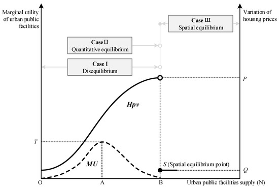
Figure 1.
Theoretical framework of the impact of urban public facility supply on inequality in housing prices.
In case I, the facility supply is between points O and B, since the supply of this facility is always lower than the citizens’ demand. If a new unit of this facility is added, its utility will always increase, which makes it always in a state of widening the variation of housing prices. In case II, when the facility supply is infinitely close to point B, the facility will reach the “quantitative equilibrium” and there is no need to continue the supply of the facility. However, the spatial equilibrium distribution cannot be achieved due to the relatively small quantity. At this time, the facility no longer generates spatial dividends and its capitalisation effect on nearby housing reaches the maximum, resulting in the largest variation of housing prices close to P. In case III, facility supply can reach point B, and such an amount of the facility will reach the “spatial equilibrium” at point S without the need to continue supply, which means that supply quantity and spatial distribution of the facility are balanced with the current needs of citizens. At point B, since the marginal utility of the facility becomes zero or a negligible minimum, the spatial dividends generated by the facility suddenly disappear and housing price variation caused by the capitalisation effect of the facility decreases to zero, causing that price variation to suddenly drop to Q. Lastly, after point B, the facility would make some appropriate adjustments such as increase, decrease, or update according to the actual demand.
4. Methodology
The current study conducts a case study to demonstrate the correctness of the theoretical framework in Section 3 which implies that urban public facilities at different supply levels have a diversified impact on the spatial inequality in the housing market. Thus the following two models are employed to identify whether the supply quantity and supply quality of urban public facilities can affect the variation of housing prices.
4.1. Hedonic Price Model
The ordinary least squares (OLS) regression model assumes data (X, Y), i = 1, 2, …, N, where X is a matrix n × p (n > p), and represent the independent and dependent variables corresponding to the ith observation, respectively, as follows:
where represents the natural logarithm of the coefficient of variation of the housing prices amongst neighbourhoods; xij represents the explanatory variable. Assuming that xij is normalised; hence, α = 0; βi denotes the estimated coefficient of model and εi is an error term.
The current study improves the hedonic price model by utilizing the theoretical framework proposed in Section 3. The selection and quantification of independent variables in the current study take into account the unbalanced spatial distribution of public facilities, which differs from the traditional way, thereby enriching the source of independent variables.
4.2. LASSO Model
Tibshirani [49] proposed the LASSO regression to solve multi-collinearity which is difficult to be solved by OLS amongst the independent variables. A coefficient matrix L1 norm is added as a penalty constraint term based on the minimisation of the residual squared sum, and the typical confidence interval and hypothesis test are no longer applicable. Lastly, the non-zero feature obtained by the LASSO model represents the optimal feature subset. Although LASSO sacrifices estimation deviation, it has good explanatory ability in parameter estimation of multiple regression. LASSO is suitable for reducing the number of parameters, selecting parameters [50] and sparse matrix [51,52]. LASSO estimates parameters by solving the following minimisation problems.
where is the tuning parameter, is the least squares estimate of , . By constantly adjusting the value of t and guaranteeing , the absolute value of regression coefficient of the insignificant variable is compressed to zero.
Efron et al. [53] invented the least angle regression (LARS) for calculations of LASSO problems. LARS is similar to the variable selection strategy of forward stepwise regression. Initially, all coefficients are zero and the algorithm finds the explanatory variable , which has the strongest correlation with the dependent variable, and moves in this direction. However, LARS does not take a complete step towards the projection of the dependent variable similar to the forward selection, it takes a step as much as possible in this direction until another independent variable appears, thereby making it as relevant as possible to current residuals. Thereafter, it continues along the direction of bisecting the angle between the first two variables and , finding variable to satisfy the strongest correlation. Thereafter, it trisects the angle amongst the first three variables to find the fourth variable. These steps are repeated until the final required independent variables are selected.
For the LASSO estimation of parameter t, Efron et al. [53] proposed a cross-validation (CV) method. CV divides the sample data into K parts and sequentially uses the kth () part as a test sample to calculate the CV residual, and the remaining K − 1 part is used to fit the model as a training sample, which is often with K = 10. Under these constraints, CV determines the most suitable tuning parameter t, thus obtaining the solution path of each coefficient and the corresponding solution value. The regularisation parameter is defined as . The prediction error estimated by the value of s on the interval (0,1) through CV is minimised by selecting . The s corresponding to the minimum CV is the final determined parameter.
4.3. Variable Selection and Quantification
The current study focuses on urban public facilities with positive externality, including urban public service facilities, urban infrastructures and natural landscape resources. The 18 types of urban public facilities selected are shown in Table 1. The current study regards urban sub-districts as the spatial research unit. Public service facilities at different supply levels are selected so as to explore whether public facilities at different levels have a diversified impact on spatial inequality in housing prices. Key primary schools, key secondary schools and key universities, grade-A tertiary hospitals, metro stations, municipal parks and river-views are regarded as high-quality public resources.

Table 1.
Definition and quantisation of variables.
Supply density and dummy variables are used to measure the supply quantity and the spatial distribution of urban public facilities, respectively, representing the status quo of the facility allocation within sub-districts. Dummy variables are also used to measure the existence of high-quality public resources due to the fact that such resources are scarce. Additionally, as far as primary school districts are concerned, there are multiple school districts within a sub-district, and the delimitation of school district boundaries also depends on the administrative boundaries of sub-districts. Therefore, choosing the existence of key primary schools within the sub-district as a quantification method of independent variables can contribute to judging whether the existence of high-quality basic education can promote the inequality in housing prices.
5. Case Study
5.1. Study Area and Data Source
Chongqing is the only municipality in Western China, and is one of most important central cities in China, as well as the economic, financial, science and technology centre in the upper reaches of the Yangtze River. The main urban area in Chongqing is the political, economic and cultural centre of the entire municipality. Its urbanization is developing fast (89.83% in 2017) and its economy has rapidly developed recently. Thus, the main urban area in Chongqing is a good sample of growing cities in China. The current study selects the metropolitan area of the main urban area planned in the Chongqing Urban and Rural Master Plan (2007–2020) as the research area, including all districts of Yuzhong, Dadukou, Jiangbei, Nan’an, Shapingba, Jiulongpo and areas of Yubei, Beibei and Ba’nan.
Urban sub-districts in Chongqing metropolitan area are taken as spatial research units. The data on housing prices were collected from Lianjia (www.lianjia.com), which is one of the most authoritative service platforms for housing information in China. From 16 to 23 October, 2018, 34,625 second-hand common commodity housing price data (unit: yuan/m2) were collected, and finally 75 sub-districts were covered as samples after processing, involving 2678 neighbourhoods. Independent variables were collected from point-of-interest data from Baidu map and quantitative data were obtained through data cleaning and ArcGIS spatial calculation. Demographic data were derived from permanent population from the national census in 2010, whereas vector data came from the Chongqing Municipal Planning Bureau (see Figure 2).
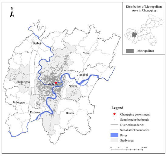
Figure 2.
Sample observations in the study area.
5.2. Principles of PublicFfacilities Allocation in the Chongqing Metropolitan Area
Allocation requirements of public facilities are based on national and local norms by governments to guide planners during the planning stage. However, the interests of suppliers vary because of the marketisation of land supply, diversification of investors and builders and unequal quantification of construction scale. Consequently, deviations in quantity or quality of facilities may emerge in the implementation process compared to the planning stage [61], currently implementing the allocation of urban public facilities is considerably more complicated than that in the formerly planned economy era in China [62]. However, it is still necessary to learn the hierarchical system of public facility allocation in the current study.
The allocation of public facilities in the Chongqing metropolitan area is mainly based on DB 50/T 543-2014 Chongqing Urban and Rural Public Service Facilities Planning Standards [63], hereinafter referred to as the ‘Chongqing standards’. The scale of residence divides the allocation of urban public facilities into four levels, namely, district, residential area, residential community and residential group. Their corresponding administrative units, planning service population and general service radius are shown in Table 2. As for public transport, location selection mainly considers where the large flow of people is located to maximise citizens’ travel convenience and efficiency [64] and so on.
Table 2.
Hierarchical allocation of public service facilities in the Chongqing metropolitan area.
5.3. Variable Descriptive Statistics
According to the ‘1000 people’ indicator for per capital possession of public facilities in the Chongqing standards, there would be 24 kindergarten students, 48 primary school students, 24 junior high school students and 18 senior high school students per 1000 people. Therefore, the proportion of students in kindergarten, primary school and secondary school within a sub-district should be 0.024, 0.048 and 0.042, respectively. This proportion is used to calculate the number of users in various schools within a sub-district. The variable of the presence of river-views is the presence of the Yangtze River or Jialing River. Variable descriptive statistics are shown in Table 3.
Table 3.
Variable descriptive statistics (sample size: N = 75).
6. Results
6.1. OLS Model Results
The estimation results of the OLS model in Table 4 show that the presence of key primary schools, grade-A tertiary hospitals, municipal parks and river-views, supply density of cultural facilities, shopping malls, supermarkets and terminal markets and banks have a significant impact on the spatial inequality in housing prices. The adjusted of this model is 0.532, thereby indicating that the fitting effect is good. However, the variance inflation factor (VIF) values of the supply densities of bus stops, cultural facilities, supermarkets and terminal markets, shopping malls and kindergartens are high, indicating that multi-collinearity amongst the explanatory variables is evident. Therefore, the LASSO model is adopted to further explain the fitting between the explanatory and dependent variables.
Table 4.
Estimation results of the OLS and LASSO models.
6.2. LASSO Model Results
The coefficient solution path of LASSO regression solved by LARS is shown in Figure 3. The abscissa is the value, the ordinate is the value of each variable parameter and the broken lines are eventually connected to the right digits to distinguish the variables. The upper digits represent the solution steps. Each line represents the coefficient change trajectory of the corresponding variable. Figure 4 shows a ten-fold CV residual variation diagram. The abscissa is the value, and the ordinate is mean squared error (MSE) value under CV. Finally, the CV calculation indicates that when the minimum MSE is 0.031, the corresponding = 0.465, = 0.640, the fitting effect of this model is good. Generally, the LASSO model validates that difference in the allocation of urban public facilities caused by the unequal supply of facilities and unbalanced spatial distribution of high-quality resources have a considerable impact on housing price variation within sub-districts.
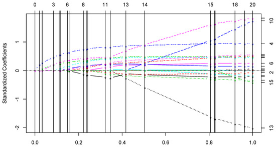
Figure 3.
LASSO coefficient βj solution path.
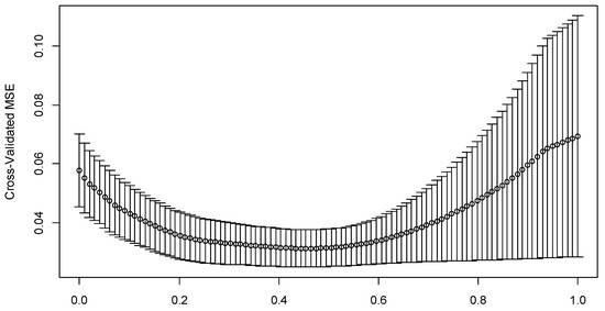
Figure 4.
Residual variation diagram under ten-fold CV.
The final parameter estimates of the LASSO model is obtained according to the determined (see Table 4). Retained are 14 variables with considerable impact. The supply densities of cultural facilities, sports facilities, shopping malls and banks have a positive impact on housing price variation. That is, the greater the supply density of these facilities, the greater spatial inequality in housing prices. Presence of key primary schools, key universities, grade-A tertiary hospitals, metro stations, municipal parks and river-views are positively correlated with the variation of housing prices. This means that the spatial inequality in housing prices will be aggravated if these high-quality resources exist within the sub-district. By contrast, the supply density of kindergartens, primary schools, secondary schools, supermarkets and terminal markets are negatively correlated with the variation of housing prices. The lower the supply density of these facilities, the higher the price inequality will be. However, presence of key high schools, supply densities of clinics and general hospitals and bus stops do not have a significant impact on the spatial inequality in housing prices.
7. Discussion
7.1. Impact of Urban Public Facility Allocation on the Spatial Inequality in Housing Prices
The current study finds that urban public facilities at different supply levels have a diversified impact on the housing market. According to the impact of urban public facility allocation on spatial inequality in housing prices, there are three available situations of facility supply, which is illustrated in the following paragraphs and eventually summarized in Table 5.
Table 5.
Summary of the characteristics of urban public facilities at different supply levels according to the impact of facility allocation on spatial inequality in housing prices.
Kindergartens, primary schools and secondary schools are basic education facilities provided by the government and supplemented by private capital. They are generally allocated on the basis of sub-districts and communities according to a small service population and small service radius so that their layout is spatially balanced. Regardless of the location of housing and educational quality, such facilities can be obtained without competition and can be equally accessed within a relatively short travel distance. Hence, additional payment for such facilities is not needed when people purchase houses. The supply of basic education facilities is at point B and beyond (see Figure 1) and their allocation achieves spatial equilibrium. However, if such facilities decrease, making youth education difficult, the availability and accessibility of educational facilities will become important, and the capitalisation effect of facilities will become considerable. Residential location becomes particularly important, compared with peripheral houses of schools, housing located close to schools will be sought after, which will exacerbate price variation. Ultimately, spatial inequality in housing prices will be exacerbated.
Supermarkets and terminal markets that provide convenience for citizens’ daily life are generally allocated according to sub-districts and communities, and their supply is based on relatively small service population and small service radius to meet the basic needs of people. Regardless of the location of housing, such services can be obtained in relatively short accessibility. One reason is that residents can obtain more of such services within a range of buffers because the higher supply density of such facilities provides plenty of alternatives. Secondly, the government stipulates that developers should provide supermarket facilities or a built environment for them because they are generally residential ancillary facilities. Hence, such facilities are generally plausible in terms of allocation efficiency and spatial distribution. Their supply is at point B and beyond (see Figure 1) and their allocation has achieved spatial equilibrium. However, if the quantity of such facilities reduces, then providing convenience for people’s daily lives will become difficult, accessibility becomes important and their capitalisation effect becomes obvious. Location will become particularly important as houses close to facilities become popular, thereby widening the variation of housing prices and eventually increasing spatial inequality in housing prices.
Shopping malls and banks as large- and medium-sized commercial facilities, large- and medium-sized cultural facilities and sports facilities fall under people’s higher-level needs. These facilities are generally allocated in accordance with cities and districts. Given their large scale and high construction cost, these facilities often serve a large population and are generally guided by the ‘1000 people’ indicator. Wherein large commercial facilities provided completely by the market are profitable, their layouts are regulated by the market and service scope is wide. Thus, the spatial distribution of such facilities is relatively unbalanced. Large- and medium-sized cultural and sports facilities that fall under public welfare facilities are mainly planned and constructed by governments with a large service radius. Compared with basic education facilities and supermarkets, the amount and per capita occupancy of these facilities are smaller. Thus their spatial distribution is extremely unbalanced. Their supply is between points O and B in Figure 1, and their allocation can only reach quantitative equilibrium. Additionally, these facilities have strong positive externality and their accessibility is related to the location of houses. Hence, housing prices around these facilities must be higher than those that are significantly distant, thereby resulting in a widening variation of housing prices. Moreover, construction costs of large- and medium-sized commercial, cultural and sports facilities are high, and their corresponding functions are relatively complete and the service population is large. Thus, it is doomed that the allocation of such facilities will not reach the spatial equilibrium point S. This find reveals that only a balance between supply and people’s demand can be achieved, but the balance of spatial distribution cannot be achieved.
High-quality and scarce public resources fall under people’s higher-level needs, their presence aggravates the contradiction of unbalanced spatial distribution. Given that key primary schools with limited service population are scarce, only families who own property rights within school districts designated by governments can be admitted to these schools [38], indicating that the availability of high-quality basic education is bound by property rights owned by citizens. Housing prices in key primary school districts are higher than that in non-school districts, which aggravates spatial inequality in housing prices. By contrast, the impact of key secondary schools on inequality in housing prices is not significant due to the fact that there is no division of school districts for secondary schools, although there is a common sense that the housing price around the secondary schools will be higher since it would be convenient for students to be close to the schools. Therefore, the housing prices around key primary schools depend more on the boundaries of school districts delineated by the government, while the housing prices around secondary schools are more dependent on market-oriented adjustment. Grade-A tertiary hospitals and metro stations are desired for convenience, and their accessibility depends on the location of houses. Key universities, municipal parks and river-views as high-quality and scarce environmental resources, and the availability of a profound humanistic environment and pleasant landscapes provided by these resources is related to the location of houses. Therefore, if people want to enjoy these high-quality public resources, then they pay additional fees for buying houses nearby. However, the influencing radius of their capitalisation effect is limited. That is, it usually decreases with the increase of distance from facilities, thereby resulting in housing price variation. Their supply is between points O and B (see Figure 1) and their allocation may be always in the disequilibrium state. Therefore, substantial housing price inequality will appear because of significant difference in the availability or accessibility of high-quality resources in an area. Moreover, Chongqing standards stipulate that public service facilities at the same level should be relatively centralized in terms of spatial layout, encouraging citizens to use various public facilities centrally to reduce travel distance. Hence, the capitalisation effects of facilities may be superimposed, thereby contributing considerably to housing price variation.
7.2. Intellectual Contributions
Under the current housing property rights system and urban public facility allocation system in China, the current study presents the following findings:
- For urban public facilities in case III that are laid out according to small administrative units, their capitalisation effects are not considerable. This finding is consistent with Wen et al. [38] who found that the capitalisation effect of basic education facility in Hangzhou was not always considerable.
- For facilities in case II that are laid out according to large administrative units, their capitalisation effects are considerable. Similarly, cultural facilities [43,57] and sports facilities [43] as well as shopping malls [60] were found that they have notable value-added effects on surrounding houses.
- The capitalisation effects of scarce and high-quality public resources in case I are considerable. Similarly, Wen et al. [38] found that the capitalisation effects of high-quality primary schools and high-quality universities are remarkable. Peng and Chiang, Wang et al. and Wen and Tao [3,11,56] found that as high-quality medical resources, the higher the spatial accessibility of grade-A tertiary hospitals are, the more evident the value-added effect on houses are. Wang et al. and Wen et al. [3,12] discovered that since the layout of metro stations is spatially unbalanced, the closer houses are to the metro station, the higher housing prices will be. Municipal parks and river-views [26,46] as high-quality and scarce landscape endowments, make an obvious value-added effect on houses in the vicinity. Lan et al. [57] also deemed that basic education is a basic necessity, and culture, sports and finance are a higher-level of needs. The current study responds to the conclusions of previous researches, which partially explain the correctness of the current study.
Additionally, Tu and Xia and Humphreys [58,59] also concluded that positive externality from sports facilities may be capitalized into residential real estate prices in US cities, which is consistent with case II of the current study. Tapsuwan et al. and Yoon [44,45] found that the presence of landscape significantly influences house sales price in Perth and Seoul, respectively, which is consistent with case III of the current study. However, the current study finds that the direction of interaction between the performance of some public facilities and housing prices is the opposite between some western countries and China. For example, housing prices have a positive impact on the quality of basic education in Paris [54] and London [55], while high-quality educational facilities can extraordinarily contribute to surrounding housing prices in China [38]. This is because the allocation of public facilities in western countries is market-oriented, while some public facilities such as the division of school districts in China are not only affected by the market but also by the considerable influence of the government. On the other hand, the supply modes of public facilities in China and the West differ because of their urbanization at different stages. Western developed countries are in the post-urbanization stage, and their current allocation of public facilities is based on bottom-up community-based governance, which is easier to meet the actual needs of residents [65]. While the allocation of public facilities in China is still planned on the basis of the service population and service scope, which is government-dominated top-down decision-making and it makes difficult to meet the heterogeneous needs of the public [30]. The current study also confirms that the impact of urban public facility allocation at different supply levels on the housing market is diversified in China.
The difference from previous researches lies in the following:
- The current study systematically analyses the impact of urban public facility allocation on their capitalisation effect, which is equivalent to summarising the conclusions of previous literature.
- The theoretical framework proposed in the current study can help form a systematic and thorough understanding of the impact of differences in urban public facility allocation on spatial inequality in housing prices: (I) For scarce and high-quality public resources that might always be in the disequilibrium state, their presence will aggravate spatial inequality in housing prices. (II) For facilities that can only achieve the quantitative equilibrium, their supply densities have a positive impact on the variation of housing prices. (III) For facilities that reach spatial equilibrium, their supply densities have a negative impact on the spatial inequality in housing prices. Thus, the current study enriches the knowledge framework and is comprehensive and universal.
8. Conclusions
The current study proposes a comprehensive and systematic theoretical framework for the impact of urban public facility allocation at different supply levels on spatial inequality in housing prices, which is verified by a case study. The conclusions are drawn as below.
- The current study finds that the supply level and supply quantity of public facilities determine whether there iss a significant difference in the accessibility or availability of facilities amongst neighbourhoods, and subsequently determines whether the capitalisation effect of such facilities is considerable, and ultimately affects the spatial inequality in housing prices. Additionally, the current study argues that the capitalisation effect of urban public facilities on housing will be considerable when the accessibility or availability of facilities has a serious stake in the location or property rights of houses. In addition, the spatial inequality in housing prices caused by the difference in accessibility or availability of public facilities is affected not only by the market, but also by the government’s planning of public facilities in China, such as the division of primary school districts.
- The case study shows that the differences in urban public facility allocation caused by an unequal supply of facilities and an unbalanced distribution of scarce and high-quality public resources have a notable impact on the spatial inequality in housing prices. The current study considers that there are three available states of urban public facility allocation, namely, disequilibrium, quantitative equilibrium and spatial equilibrium: (I) The scarce and high-quality public resources that fall under people’s higher-level needs may always be in the disequilibrium state, their availability or accessibility is bound by property rights or related to the location of housing. The capitalisation effect of such resources is substantial, and their presence will aggravate spatial inequality in housing prices, such as key primary schools, key universities, grade-A tertiary hospitals, metro stations, municipal parks and river-views. (II) Facilities laid out on the basis of large administrative units (e.g., cities and districts) supplied in small amounts but with a large service population and wide service scope, fall under people’s higher-level needs. The availability of these facilities, such as shopping malls, banks, large- and medium-sized cultural facilities and sports facilities depend on the location of housing. The supply of such facilities can only reach the quantitative equilibrium (only a balance between supply and people’s demand can be achieved, but the balance of spatial distribution cannot be achieved) makes their capitalisation effect considerable, and their supply densities have a positive impact on the spatial inequality in housing prices. (III) Facilities, such as kindergartens, primary schools, secondary schools, supermarkets and terminal markets that are laid out according to small administrative units (e.g., sub-districts and communities) with a small service radius and a small service population, fall under people’s basic needs. The supply of such facilities that reach the spatial equilibrium makes their capitalisation negligible, and their supply densities have a negative impact on the spatial inequality in housing prices. Therefore, it is reasonable to argue that the impact of urban public facilities at different supply levels on the housing market is diversified.
- Additionally, the current study finds that the impact of public facility allocation on housing price inequality has nothing to do with who the main supplier of the facility is.
The current study has four limitations:
- Because of the limited availability of data, the current study omits differences amongst neighbourhoods and the independent variables selected do not cover all types of urban public facilities. In addition, the research units selected in this study are divided according to the administrative boundaries commonly used in China’s statistics. However, the actual use of public facilities may not be strictly in accordance with the administrative boundaries, so the current results may deviate from the actual situation, and big data accessible on the Internet is expected to be used for further exploration.
- The LASSO model is sensitive to noise, thereby causing inevitable weaknesses.
- Given that China’s seventh census in 2020 has yet to commence, the current study uses the sixth census data and administrative boundary vector data in 2010. Thus, deviations from the current social situation may exist.
- The research unit chosen in the current study may be limited and further exploration is needed by using different research units, but it is sufficient to prove that the theoretical framework proposed in this study can reflect the real trend and has a certain value. The next step is to refine and improve these shortcomings.
9. Note
- District: “qu” in Mandarin Chinese. It is an administrative jurisdiction unit within Chinese cities.
- Sub-district: “jiedao” in Mandarin Chinese. It is an administrative jurisdiction unit within Chinese cities.
- Community: “shequ” in Mandarin Chinese. It refers to the social community composed of people living in a certain geographical area, which is the most basic unit of social organisms.
- Neighbourhood: “xiaoqu” in Mandarin Chinese. It refers to a large number of houses with a relatively independent living environment in a certain area of the city. It is equipped with a set of living service facilities, which are generally constructed by one developer and has similarities in attributes such as quality and age. Thus, the variation of housing prices within the neighbourhood is circumvented to an extent.
According to the size of an urban area, it is generally the District > Sub-district > Community > Neighbourhood.
Author Contributions
Conceptualization, T.Z. and C.M.; Data curation, L.Z.; Methodology, L.Z.; Writing—original draft, L.Z.; Writing—review & editing, T.Z. and C.M.
Funding
This research was funded by the National Social Science Foundation of China (grant number 19GBL278) and the National Natural Science Foundation of China (grant number 71673285).
Conflicts of Interest
The authors declare no conflict of interest.
References
- Knox, P.; Pinch, S. Urban Social Geography: An Introduction, 6th ed.; Routledge: London, UK, 2009. [Google Scholar]
- Lineberry, R.L. Equality and Urban Policy: The Distribution of Municipal Public Services; Beverly Hills: London, UK, 1977. [Google Scholar]
- Wang, Y.; Feng, S.; Deng, Z.; Cheng, S.; Feng, S. Transit premium and rent segmentation: A spatial quantile hedonic analysis of Shanghai Metro. Transp. Policy 2016, 51, 61–69. [Google Scholar] [CrossRef]
- Sheppard, S. Hedonic analysis of housing markets. In Handbook of Regional and Urban Economics; Elsevier: Amsterdam, The Netherlands, 1999; Volume 3, pp. 1595–1635. [Google Scholar]
- Demsetz, H. Toward a Theory of Property Rights. In Classic Papers in Natural Resource Economics; Palgrave Macmillan: London, UK, 1974. [Google Scholar]
- Almohamad, H.; Knaack, A.L.; Habib, B.M. Assessing Spatial Equity and Accessibility of Public Green Spaces in Aleppo City, Syria. Forests 2018, 9, 706. [Google Scholar] [CrossRef]
- Lindsey, G.; Maraj, M.; Kuan, S. Access, Equity, and Urban Greenways: An Exploratory Investigation. Prof. Geogr. 2001, 53, 332–346. [Google Scholar] [CrossRef]
- Wolch, J.; Wilson, J.P.; Fehrenbach, J. Parks and Park Funding in Los Angeles: An Equity-Mapping Analysis. Urban Geogr. 2005, 26, 4–35. [Google Scholar] [CrossRef]
- Downey, L.; Dubois, S.; Hawkins, B.; Walker, M. Environmental Inequality in Metropolitan America. Sociol. Spectr. 2006, 26, 21–41. [Google Scholar] [CrossRef]
- Yoon, D.; Kang, J.; Park, J. Exploring Environmental Inequity in South Korea: An Analysis of the Distribution of Toxic Release Inventory (TRI) Facilities and Toxic Releases. Sustainability 2017, 9, 1886. [Google Scholar] [CrossRef]
- Wen, H.; Tao, Y. Polycentric urban structure and housing price in the transitional China: Evidence from Hangzhou. Habitat Int. 2015, 46, 138–146. [Google Scholar] [CrossRef]
- Wen, H.; Gui, Z.; Tian, C.; Xiao, Y.; Fang, L. Subway Opening, Traffic Accessibility, and Housing Prices: A Quantile Hedonic Analysis in Hangzhou, China. Sustainability 2018, 10, 2254. [Google Scholar] [CrossRef]
- Dajani, J.S. Cost Studies of Urban Public Services. Land Econ. 1973, 49, 479. [Google Scholar] [CrossRef]
- Cooper, L. Location-Allocation Problems. Oper. Res. 1963, 11, 331–343. [Google Scholar] [CrossRef]
- Teitz, M.B. Toward a theory of urban public facility location. Pap. Reg. Sci. 1968, 21, 35–51. [Google Scholar] [CrossRef]
- Jones, B.D.; Kaufman, C. The Distribution of Urban Public Services: A Preliminary Model. Adm. Soc. 1974, 6, 337–360. [Google Scholar] [CrossRef]
- Burdziej, J. Using hexagonal grids and network analysis for spatial accessibility assessment in urban environments—A case study of public amenities in Toruń. Misc. Geogr. 2019, 23, 99–110. [Google Scholar] [CrossRef]
- Zhao, Y.; Zhang, G.; Lin, T.; Liu, X.; Liu, J.; Lin, M.; Ye, H.; Kong, L. Towards Sustainable Urban Communities: A Composite Spatial Accessibility Assessment for Residential Suitability Based on Network Big Data. Sustainability 2018, 10, 4767. [Google Scholar] [CrossRef]
- Apparicio, P.; Seguin, A.-M. Measuring the Accessibility of Services and Facilities for Residents of Public Housing in Montreal. Urban Stud. 2006, 43, 187–211. [Google Scholar] [CrossRef]
- Taleai, M.; Sliuzas, R.; Flacke, J. An integrated framework to evaluate the equity of urban public facilities using spatial multi-criteria analysis. Cities 2014, 40, 56–69. [Google Scholar] [CrossRef]
- Dadashpoor, H.; Rostami, F. Measuring spatial proportionality between service availability, accessibility and mobility: Empirical evidence using spatial equity approach in Iran. J. Transp. Geogr. 2017, 65, 44–55. [Google Scholar] [CrossRef]
- DeRuyter, G. Evaluating spatial inequality in pre-schools in Ghent, Belgium by accessibility and service area analysis with GIS. In Proceedings of the 13th International Multidisciplinary Scientific GeoConference-SGEM, Albena, Bulgary, 16–22 June 2013. [Google Scholar]
- Lu, C.; Zhang, Z.; Lan, X. Impact of China’s referral reform on the equity and spatial accessibility of healthcare resources: A case study of Beijing. Soc. Sci. Med. 2019, 235, 112386. [Google Scholar] [CrossRef]
- Zheng, Z.; Xia, H.; Ambinakudige, S.; Qin, Y.; Li, Y.; Xie, Z.; Zhang, L.; Gu, H. Spatial Accessibility to Hospitals Based on Web Mapping API: An Empirical Study in Kaifeng, China. Sustainability 2019, 11, 1160. [Google Scholar] [CrossRef]
- Hu, S.; Song, W.; Li, C.; Lu, J. The Spatial Equity of Nursing Homes in Changchun: A Multi-Trip Modes Analysis. ISPRS Int. J. Geo-Inf. 2019, 8, 223. [Google Scholar] [CrossRef]
- Kong, F.; Yin, H.; Nakagoshi, N. Using GIS and landscape metrics in the hedonic price modeling of the amenity value of urban green space: A case study in Jinan City, China. Landsc. Urban Plan. 2007, 79, 240–252. [Google Scholar] [CrossRef]
- Chen, T.; Hui, E.C.-M.; Lang, W.; Tao, L. People, recreational facility and physical activity: New-type urbanization planning for the healthy communities in China. Habitat Int. 2016, 58, 12–22. [Google Scholar] [CrossRef]
- Scott, D.; Jackson, E.L. Factors that limit and strategies that might encourage people’s use of public parks. J. Park Recreat. Adm. 1996, 14, 1–17. [Google Scholar]
- Stanley, B.W.; Dennehy, T.J.; Smith, M.E.; Stark, B.L.; York, A.M.; Cowgill, G.L.; Novic, J.; Ek, J. Service Access in Premodern Cities: An Exploratory Comparison of Spatial Equity. J. Urban Hist. 2016, 42, 121–144. [Google Scholar] [CrossRef]
- Gao, J.B.; Zhou, C.S.; Jiang, H.Y.; Chang-Dong, Y.E. The Research on the Spatial Differentiation of the Urban Public Service Facilites Distribution in Guangzhou. Hum. Geogr. 2010, 25, 78–83. (In Chinese) [Google Scholar]
- Hart, J.T. The inverse care law. Lancet 1971, 297, 405–412. [Google Scholar] [CrossRef]
- Rahman, M.; Dhaka, B.; Neema, M.N. A GIS Based Integrated Approach to Measure the Spatial Equity of Community Facilities of Bangladesh. Aims Geosci. 2015, 1, 21–40. [Google Scholar] [CrossRef]
- Bondarabady, H.A.; Khavarian-Garmsir, A.R. An analyses of the role of socio-economic classes in the spatial organization (a case study of Yazd, Iran). J. Archaeol. Sci. Rep. 2019, 25, 486–497. [Google Scholar] [CrossRef]
- Heynen, N.; Perkins, H.A.; Roy, P. The Political Ecology of Uneven Urban Green Space. Urban Aff. Rev. 2006, 42, 3–25. [Google Scholar] [CrossRef]
- Comber, A.; Brunsdon, C.; Green, E. Using a GIS-based network analysis to determine urban greenspace accessibility for different ethnic and religious groups. Landsc. Urban Plan. 2008, 86, 103–114. [Google Scholar] [CrossRef]
- Pearce, J.; Witten, K.; Hiscock, R.; Blakely, T. Are socially disadvantaged neighbourhoods deprived of health-related community resources? Int. J. Epidemiol. 2007, 36, 348–355. [Google Scholar] [CrossRef] [PubMed]
- Tahmasbi, B.; Mansourianfar, M.H.; Haghshenas, H.; Kim, I. Multimodal accessibility-based equity assessment of urban public facilities distribution. Sustain. Cities Soc. 2019, 49, 101633. [Google Scholar] [CrossRef]
- Wen, H.; Xiao, Y.; Hui, E.C.; Zhang, L. Education quality, accessibility, and housing price: Does spatial heterogeneity exist in education capitalization? Habitat Int. 2018, 78, 68–82. [Google Scholar] [CrossRef]
- Munoz-Raskin, R. Walking accessibility to bus rapid transit: Does it affect property values? The case of Bogotá, Colombia. Transp. Policy 2010, 17, 72–84. [Google Scholar] [CrossRef]
- Cervero, R.; Kang, C.D. Bus rapid transit impacts on land uses and land values in Seoul, Korea. Transp. Policy 2011, 18, 102–116. [Google Scholar] [CrossRef]
- Mulley, C.; Tsai, C.-H.P. When and how much does new transport infrastructure add to property values? Evidence from the bus rapid transit system in Sydney, Australia. Transp. Policy 2016, 51, 15–23. [Google Scholar] [CrossRef]
- Wang, Y.; Potoglou, D.; Orford, S.; Gong, Y. Bus stop, property price and land value tax: A multilevel hedonic analysis with quantile calibration. Land Use Policy 2015, 42, 381–391. [Google Scholar] [CrossRef]
- Yang, L.; Wang, B.; Zhou, J.; Wang, X. Walking accessibility and property prices. Transp. Res. Part D Transp. Environ. 2018, 62, 551–562. [Google Scholar] [CrossRef]
- Tapsuwan, S.; Ingram, G.; Burton, M.; Brennan, D. Capitalized amenity value of urban wetlands: A hedonic property price approach to urban wetlands in Perth, Western Australia. Aust. J. Agric. Resour. Econ. 2010, 53, 527–545. [Google Scholar] [CrossRef]
- Yoon, H. When and where do we see the proximity effect of a new park? A case study of the Dream Forest in Seoul, Korea. J. Environ. Plan. Manag. 2018, 61, 1113–1136. [Google Scholar] [CrossRef]
- Wen, H.; Xiao, Y.; Zhang, L. Spatial effect of river landscape on housing price: An empirical study on the Grand Canal in Hangzhou, China. Habitat Int. 2017, 63, 34–44. [Google Scholar] [CrossRef]
- Mankiw, N.G. Principles of Economics, 6th ed.; South-Western Cengage Learning: Boston, MA, USA, 2012. [Google Scholar]
- Oates, W.E. The Effects of Property Taxes and Local Public Spending on Property Values: An Empirical Study of Tax Capitalization and the Tiebout Hypothesis. J. Political Econ. 1969, 77, 957–971. [Google Scholar] [CrossRef]
- Tibshirani, R. Regression Shrinkage and Selection via the Lasso. J. R. Stat. Soc. Ser. B (Methodol.) 1996, 58, 267–288. [Google Scholar] [CrossRef]
- Oladunni, T.; Sharma, S.; Tiwang, R. A Spatio-Temporal Hedonic House Regression Model. In Proceedings of the 16th IEEE International Conference on Machine Learning and Applications (ICMLA), Cancun, Mexico, 18–21 December 2017; pp. 607–612. [Google Scholar]
- Huang, Y.-Q.; Liang, C.-H.; He, L.; Tian, J.; Liang, C.-S.; Chen, X.; Ma, Z.-L.; Liu, Z.-Y. Development and Validation of a Radiomics Nomogram for Preoperative Prediction of Lymph Node Metastasis in Colorectal Cancer. J. Clin. Oncol. 2016, 34, 2157–2164. [Google Scholar] [CrossRef]
- Wu, S.; Zheng, J.; Li, Y.; Yu, H.; Shi, S.; Xie, W.; Liu, H.; Su, Y.; Huang, J.; Lin, T. A Radiomics Nomogram for the Preoperative Prediction of Lymph Node Metastasis in Bladder Cancer. Clin. Cancer Res. 2017, 23, 6904–6911. [Google Scholar] [CrossRef]
- Efron, B.; Hastie, T.; Johnstone, I.; Tibshirani, R. Least Angle Regression. Ann. Stat. 2004, 32, 407–451. [Google Scholar]
- Fack, G.; Grenet, J. When do better schools raise housing prices? Evidence from Paris public and private schools. J. Public Econ. 2010, 94, 59–77. [Google Scholar] [CrossRef]
- Machin, S. Houses and schools: Valuation of school quality through the housing market. Labour Econ. 2011, 18, 723–729. [Google Scholar] [CrossRef]
- Peng, T.-C.; Chiang, Y.-H. The non-linearity of hospitals’ proximity on property prices: Experiences from Taipei, Taiwan. J. Prop. Res. 2015, 32, 341–361. [Google Scholar] [CrossRef]
- Lan, F.; Wu, Q.; Zhou, T.; Da, H. Spatial Effects of Public Service Facilities Accessibility on Housing Prices: A Case Study of Xi’an, China. Sustainability 2018, 10, 4503. [Google Scholar] [CrossRef]
- Tu, C.C. How Does a New Sports Stadium Affect Housing Values? The Case of FedEx Field. Land Econ. 2005, 81, 379–395. [Google Scholar] [CrossRef]
- Xia, F.; Humphreys, B.R. The impact of professional sports facilities on housing values: Evidence from census block group data. City Culture & Society 2012, 3, 189–200. [Google Scholar]
- Zhang, L.; Zhou, J.; Hui, E.C.M.; Wen, H. The effects of a shopping mall on housing prices: A case study in Hangzhou. Int. J. Strateg. Prop. Manag. 2019, 23, 65–80. [Google Scholar] [CrossRef]
- Zhou, C.S.; Gao, J.B. Provision Pattern of Urban Public Service Facilities and its Formation Mechanism During Transitional China. Sci. Geogr. Sin. 2011, 31, 272–279. (In Chinese) [Google Scholar]
- Yu, J. China’s Public Service System: Developments of Social Policy, Institution and Mechanism. Acad. Mon. 2011, 43, 5–17. (In Chinese) [Google Scholar]
- Chongqing Planning and Design Institute DB 50/T 543–2014 Chongqing Urban and Rural Public Service Facilities Planning Standards; China Architecture & Building Press: Beijing, China, 2014. (In Chinese)
- Liu, X.; Macedo, J.; Zhou, T.; Shen, L.; Liao, Y.; Zhou, Y. Evaluation of the utility efficiency of subway stations based on spatial information from public social media. Habitat Int. 2018, 79, 10–17. [Google Scholar] [CrossRef]
- Michalos, A.C.; Zumbo, B.D. Public Services and the Quality of Life. Soc. Indic. Res. 1999, 48, 125–157. [Google Scholar] [CrossRef]


© 2019 by the authors. Licensee MDPI, Basel, Switzerland. This article is an open access article distributed under the terms and conditions of the Creative Commons Attribution (CC BY) license (http://creativecommons.org/licenses/by/4.0/).