Article

Optimal Logistics Control of an Omnichannel Supply Chain

School of Automation, Beijing University of Posts and Telecommunications, Beijing 100876, China
*
Authors to whom correspondence should be addressed.
Sustainability 2019, 11(21), 6014; https://doi.org/10.3390/su11216014
Submission received: 29 September 2019 / Revised: 27 October 2019 / Accepted: 27 October 2019 / Published: 29 October 2019

Abstract

:
This paper aims to find the best way to control logistics in an omnichannel supply chain (OSC). For this purpose, two steps of work were carried out around case-based reasoning (CBR). In the first step, the combined feedback which proved stability was selected to control logistics in the single node, while the variational method and the virtual siphon were combined to determine the optimal control curve. There is a linear part and a nonlinear part in the combined feedback. The new method of storing data mode is “data turning to picture”. In the second step, image features were extracted by the hybrid method of SURF-GoogLeNet and used for case matching via the grey cloud method. SURF-GoogLeNet was firstly used to update the weight proportion of the defect points in the whole image via the speeded up robust features (SURF) method and secondly to self-extract features using the GoogLeNet method. Finally, the effectiveness of the proposed methods was verified through experiments. The research findings shed new light on the management of supply chains.

1. Introduction

Supply chain management involves various activities and processes, including planning, coordination, operation, control, and optimization of the entire supply chain system. With the proliferation of computers and smartphones, a brand-new type of supply chain has emerged, which is known as the omnichannel supply chain (OSC) [1]. OSC means the full integration of online and offline marketing channels. It is not a simple superposition of multiple channels. It is a concept which was proposed after 2015, and it integrates the concept of artificial intelligence and meets the needs of customers in real time [2,3]. OSC management aims to deliver high-quality products to customers at the right place, the right time, and minimal total cost [4,5]. Recently, optimal logistics control has become the focal point of research into supply chain management. Some of the representative studies are reviewed below.
Alfares et al. [6] combined the quality control and inventory control into an integrated mathematical model and found the optimal solution of the model for three different levels of supply chains. Sarkar et al. [7] maintained the optimal production level of the supply chain at a certain time interval and determined the global optimal production rate using the game theory. White et al. [8] combined the extended labor model and the vendor-managed inventory (VMI) model and obtained the optimal solution of the inventory through the analysis of the combined system. Taking distributors as an investment model, Chang et al. [9] determined the optimal inventory level by thoroughly examining the cost, demand, and price variation. Sadeghi et al. [10] constructed a dual-objective model with a single manufacturer, a single supplier, and multiple retailers and proposed a hybrid bats algorithm to approximate the optimal solution to the model. Nevertheless, none of the above control models take account of the feedback in the closed loop, which is the basis of control. One of the popular strategies for supply chain management is case-based reasoning (CBR). CBR was proposed by Roger Schank of Yale University in 1982 in dynamic memory. It is an important knowledge-based problem solving and learning method in the field of artificial intelligence (AI). It solves problems by reusing or modifying previous solutions to similar problems. There are two ways to improve CBR: using the standard optimal solution in case library; and reducing the data size and increasing the computing speed through case matching [11]. Over the years, CBR has been adopted for supply chain management, independently or in association with radio frequency identification (RFID).
Concerning the independent use of CBR in supply chain management, Zhao et al. [12] probed deep into the defects of supplier selection methods in the supply chain of oil companies, took the weight of information entropy as the objective attribute of the case library, and disclosed the relationship between potential rules and the backpropagation (BP) neural network. Germani et al. [13] employed the CBR for emergency management and identified new cases according to the existing rules; this method can rapidly pinpoint the advantages and problems of supply chain systems. CBR has been fully integrated with RFID by many scholars, namely, Choy et al., and applied to the following five aspects of supply chain management: case logistics resource management system [14], food distribution control for reception activities [15], temperature control in wine storage facilities [16], acquisition of inventory data and decision making [15], and the selection of fabric for new products [17]. The application enhances the resource management and competitiveness of enterprises in these areas. However, these studies ignore case matching and hard disk data compression, despite attempts to improve algorithm efficiency. As mentioned before, case matching is an important way to improve CBR, while hard disk data compression needs to be considered in the process of CBR, due to the huge amount of data generated in the supply chain network.
In light of the above, this study explored how to improve the logistics management of the omnichannel supply chain. Closed-loop control in OSC logistics was considered, and the siphon phenomenon was mapped the logistics deployment phenomenon of OSC. The new method of compressed sensing mode is “data turning to picture”. To speed up case processing, the optimal logistics case matching of OSC was improved through the modification of the cloud model method in CBR. The research was implemented in two steps: case adjustment and case description/matching. In the first step, the combined feedback which proved stability was selected to control logistics in the single node, while the variational method and the virtual siphon were combined to determine the optimal control curve. In the second step, image features were extracted using the hybrid method of SURF-GoogLeNet and used for case matching via the grey cloud method. SURF-GoogLeNet is a new method of image feature extraction. There are two parts in the new method. Firstly, the SURF method is used to update the weight proportion of the defect points in whole image. Secondly, the features of the processed image are self-extracted via the GoogLeNet method. Finally, the effectiveness of the proposed methods was verified through experiments.

2. The Case Adjustment of the Case Library in CBR of the OSC

There are three sales channels in the OSC, namely, online, offline, and mobile [18]. The information of any channel is displayed in real-time in the OSC operating system. For example, if a customer places an order online but the required item is not in the logistics center but the end store, the terminal store will carry out order processing and logistics distribution quickly according to the order information. This adjustment process can be naturally solved by the CBR.
In 1982, Schank [19] put forward the idea of the CBR, a knowledge-based method in the field of artificial intelligence. The CBR solves problems using the original or modified plans of similar problems. As shown in Figure 1 below, CBR involves five steps: representation, retrieval, reusing, revision, and retaining [20].
In this paper, CBR was improved through case adjustment and case description/matching. For case adjustment, stable combined feedback was introduced to the case library, the updated case library was solved via the variational method, and a virtual siphon was proposed to determine the value of endpoints. The resulting data were stored in the form of images. For case description/matching, the case was matched with hybrid image features, including intrinsic features and texture features, via the grey-cloud method.
The feedback and solution of the OSC depend on the analysis of each node in the network. Here, the combination of linear and nonlinear feedbacks, i.e., the combined feedback, was selected to control the logistics of each node [21]. The stability of the combined feedback is well proven [22]. Further, the optimal control curve and endpoint value were solved, respectively, by the variational method and the virtual siphon method. The results were saved in the form of images.

2.1. Combined Feedback Model

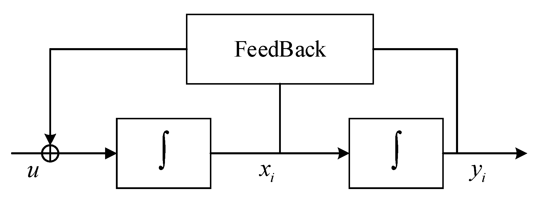
In the OSC, the state of inventory is measured by change rate, change quantity, and total amount. Integral relationships exist between change rate and change quantity, and between change quantity and total amount. Hence, the block diagram of the combined feedback device was designed (Figure 2).
The combined feedback device, with both linear and nonlinear features, can effectively enhance the control accuracy. The device can be expressed as:
Γ ( x i , y i ) = K p x i + K d y i + K p y i ( e x i + e y i )
The linear part and nonlinear part of the device can be expressed as:
Γ ( x i , y i ) = Γ 1 ( x i , y i ) + Γ 2 ( x i , y i )
The linear part Γ 1 ( x 1 , x 2 ) can also be expressed as:
Γ 1 ( x i , y i ) = K p x i + K d y i
where Kp and Kd are positive definite matrices of i × i.
The nonlinear part Γ 2 ( x i , y i ) can also be expressed as:
Γ 2 ( x i , y i ) = K p y i ( e x i + e y i )
where Kp and Kd satisfy the following condition:
[ 0 I K d K p ] T P + P [ 0 I K d K p ] = Q
To simplify the calculation, Kp, Kd, and Q are given. Kp and Kd are i × i known positive definite matrices. At the same time, Kp and Kd are diagonal matrices. Q is a given positive definite matrix of 2i × 2i.
The combined feedback device must be stable before being used for subsequent analysis [23]. According to Equation (2), the state equations of the device can be derived as:
{ y ˙ i = x i x ˙ i = Γ ( x i , y i )
[ y ˙ i x ˙ i ] = [ 0 0 ] [ y i x i ] = [ 0 0 ]
The following equation can be derived from Equation (7):
[ y ˙ i x ˙ i ] = [ 0 I K p 1 K d 1 ] [ y i x i ] [ 0 0 K p 2 K d 2 ] [ x i ( e x i + e y i ) 0 ]
Then, the Lyapunov function can be defined as:
V ( x i , y i ) = [ x i y i ] T P [ x i y i ]
Since P must be a positive definite matrix, we have P 0 .
The derivation of Equation (9) can be expressed as:
d d t V ( x i , y i ) = [ y i x i ] T P [ y ˙ i x ˙ i ] + [ y ˙ i x ˙ i ] T P [ y i x i ] = [ y i x i ] T Q [ y i x i ] [ y i x i ] T Q [ x i ( e x i + e y i ) 0 ]
where [ y i x i ] = 0 d d t V ( x i , y i ) = 0 . Therefore, the point of [ y i x i ] = 0 is the equilibrium point. Since d d t V ( x i , y i ) 0 , the system is stable. Then, the situation of [ y i x i ] 0 d d t V ( x i , y i ) 0 is non-existent and the situation of [ y i x i ] V ( x i , y i ) is existent. The system is proven as progressively stable and large-scale progressively stable.

2.2. Optimal Control Solution

The next step is to solve the optimal control curve of the established combined feedback model. This curve can be solved by various approaches, such as the traditional variational method [24,25] and the popular strategies like direct methods and indirect methods. The direct methods include the shooting method and multiple shooting method [26,27], while the indirect methods include the discrete mechanics and optimal control (DMOC) method and Gauss pseudospectral method [28,29,30]. Here, the traditional method is adopted for its robustness and stability.

2.2.1. Solution of the Optimal Control Curve

The state variables can be defined as:
{ y ˙ i ( t ) = x i ( t ) x ˙ i ( t ) = Γ ( x i ( t ) , y i ( t ) ) + u ( t )
To solve the optimal control curve, two optimal objective functions were selected below:
The optimal time:
J 1 = t f
The optimal energy:
J 2 = 1 2 t 0 t f u T ( t ) u ( t ) d t
The above two objectives can be combined to form a comprehensive optimal objective:
J = J 1 + J 2
Thus, the comprehensive optimal objective function can be expressed as:
J = t f + 1 2 0 t f u T ( t ) u ( t ) d t
According to the optimal solution of the variational method, the Hamiltonian function can be constructed as:
H = 1 2 u ( t ) + λ 1 ( t ) x ˙ ( t ) + λ 2 ( t ) y ˙ ( t )
Then, the co-state equations and state equations can be established as:
H u i = 0
λ ˙ 1 i = H x i , λ ˙ 2 i = H y i

2.2.2. Solution of Endpoint Value

During transaction, the supply chain faces an allocation problem between the three sales channels. The nodes with more materials will automatically supplement those with fewer materials. This automatic adjustment bears resemblance to the siphonic effect [31], which is the result of height difference between liquid surfaces. Pascal’s law p = ρgh applies to the siphonic process, in which the effect of atmospheric pressure can be expressed as P-ρgh. Here, the automatic balancing of materials in the supply chain is analogized as a virtual siphon:
(1)
The atmospheric pressure, a driving force of siphonage, was compared to the emergency level in the OSC material balance. Considering the positive correlation between the pressure and flow rate, the emergency level was assumed to be positively proportional to the inventory coordination speed between multiple channels.
(2)
The gravitational acceleration, another driver of liquid flow in siphonage, was compared to the logistics speed in the OSC material balance. The speed was assumed to be fixed under the same conditions, as the gravitational acceleration is stabilized at 9.8.
(3)
The liquid density, a determinant of flow rate in siphonage, was compared to the material price in the OSC material balance. The price was assumed to be positively proportional to the level of care and negatively to logistics speed, in light of the relationship between liquid density and flow rate.
(4)
The height difference in siphonage, a source of liquid pressure, was compared to the difference in material state in the OSC material balance. The relationship between material state and balance was assumed according to the negative correlation between the height of liquid level and the flow rate.
In each sales channel, the inventory state is measured by change rate, change quantity, and total amount. From the start to the end of the siphonage, the relationship between these three variables can be expressed as:
{ x ˙ i ( t 0 ) = 0 , x ˙ i ( t f ) = 0 x i ( t 0 ) = 0 , x i ( t f ) = 0 y i ( t 0 ) = A i , x i ( t f ) = a v e r a g e ( A i )

2.3. Saving as Images

For data compression, the logistics information of the OSC was saved as images under the following assumptions: There are three sales channels, namely, offline, online, and mobile; each channel has multiple nodes, which represent players like manufacturer, distributor, and customer; the information of each node varies with time. A total of five steps were needed to save the OSC logistics information in the form of images:
Step 1: The offline, online, and mobile channels were analogized as the R, G, and B light beams in an image. The logistics value of each node was normalized to the interval [ 0 255 ] .
Step 2: The points on the x-axis of the saved image were uniformly distributed, continuous time points, each of which represents a unit of time.
Step 3: The points on the y-axis of the saved image were corresponding to the nodes in the OSC.
Step 4: The information of the OSC was divided into a series of continuous images by date.
Step 5: The images were saved in a .jpg format or .bmp format.
The key to the CBR lies in the retrieval of cases from the case library, in which the information is saved as a multiframe image. Here, case retrieval is completed through the following steps:
Step 1: The features were extracted from the original and new cases in the case library, both of which were saved as images.
Step 2: The features of new cases were compared with those of the original ones in the library. The similarity was measured via the Euclidean distance method. Case matching was performed by experts.
Step 3: The matched cases were retrieved from the library and applied in actual work.
Step 4: New cases were added to the library after case retrieval. With the elapse of time, the library will be constantly updated.
The first two steps are explained in detail in the next section.

3. Case Description and Matching in CBR of the OSC

The features of the saved images were extracted via the hybrid method called SURF-GoogLeNet, and then case matching was conducted via the grey-cloud method.

3.1. Feature Extraction

The features of an image fall into five main categories: color features, texture features, shape features, intrinsic features, and spatial features. It is widely agreed that image properties can only be determined accurately based on more than one type of features. Hence, both intrinsic features and texture features were extracted in this paper. This idea came from the hybrid processing of image shooting and drawing in additive manufacturing (AM) [32,33,34,35]. The intrinsic features were extracted via the deep learning method GoogleLeNet, while the texture features were extracted via the SURF method.

3.1.1. Extraction of Intrinsic Features

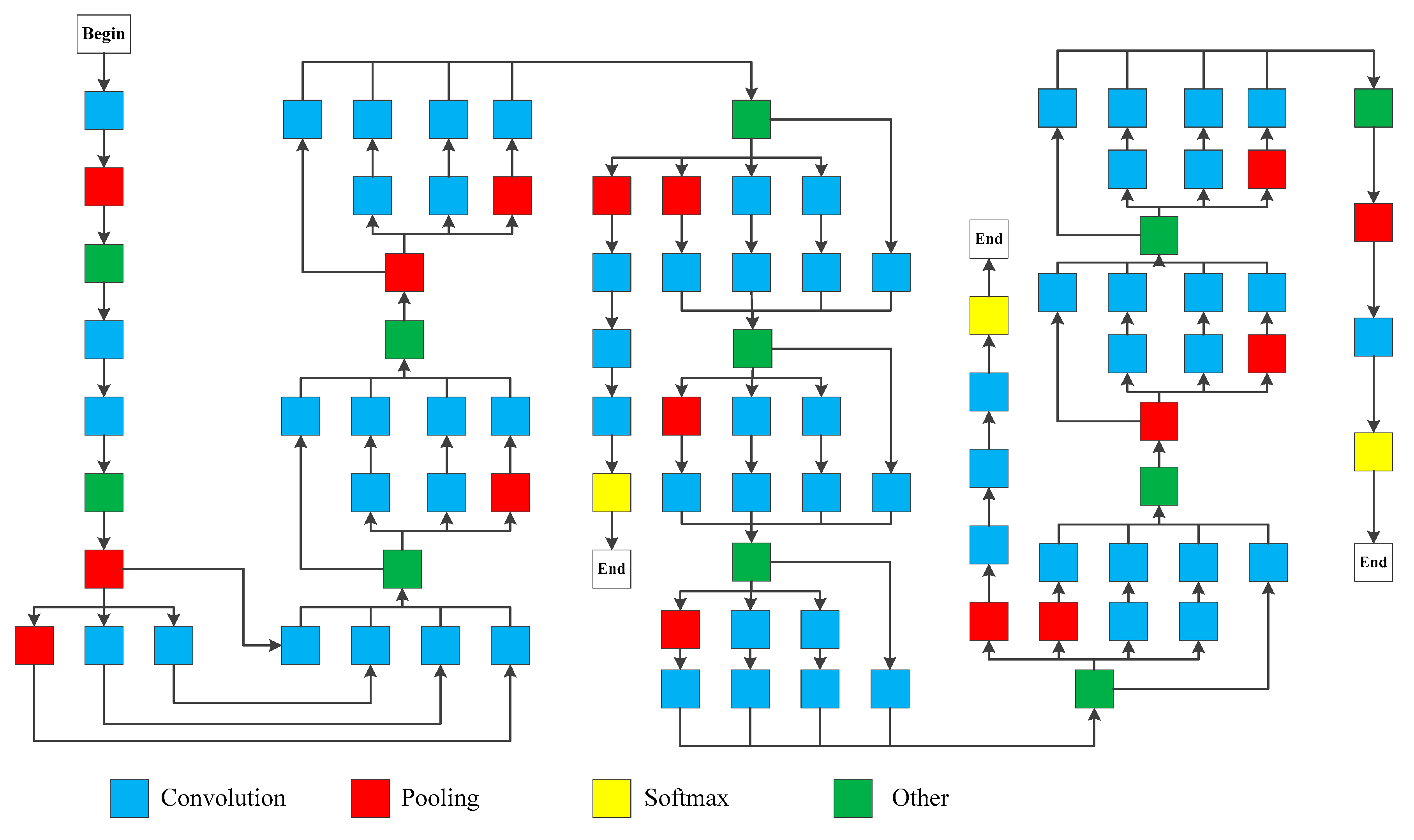
GoogLeNet is a deep convolutional neural network (CNN) model designed by Google [36,37]. As shown in Figure 3, the network consists of 22 layers.
Through sparse learning, the network scale is enlarged by adjusting the parameters of a sparse network. GoogLeNet can automatically extract the intrinsic features from images, thanks to the following attributes:
(1)
It is easy to add and modify images through the modular structure of GoogLeNet.
(2)
The fully-connected layer is replaced with average pooling, pushing up the accuracy by 0.6%.
(3)
Despite the removal of the fully-connected layer, the concept of dropout is retained in the network.
(4)
Two additional modules are added to prevent gradient disappearance.
Here, GoogLeNet is employed to extract the intrinsic features from the saved images. The extracted features were combined with the contour features of the target images before receiving the confidence test.

3.1.2. Extraction of Texture Features

Compared with the scale-invariant feature transform (SIFT), the SURF is a simple and fast algorithm to extract interest points and describe eigenvectors [38,39]. The SURF method contains five steps, namely, constructing a Hessian matrix, calculating eigenvalue, constructing a Gaussian pyramid, determining the principal direction of a feature point, locating feature points, and constructing feature descriptors.
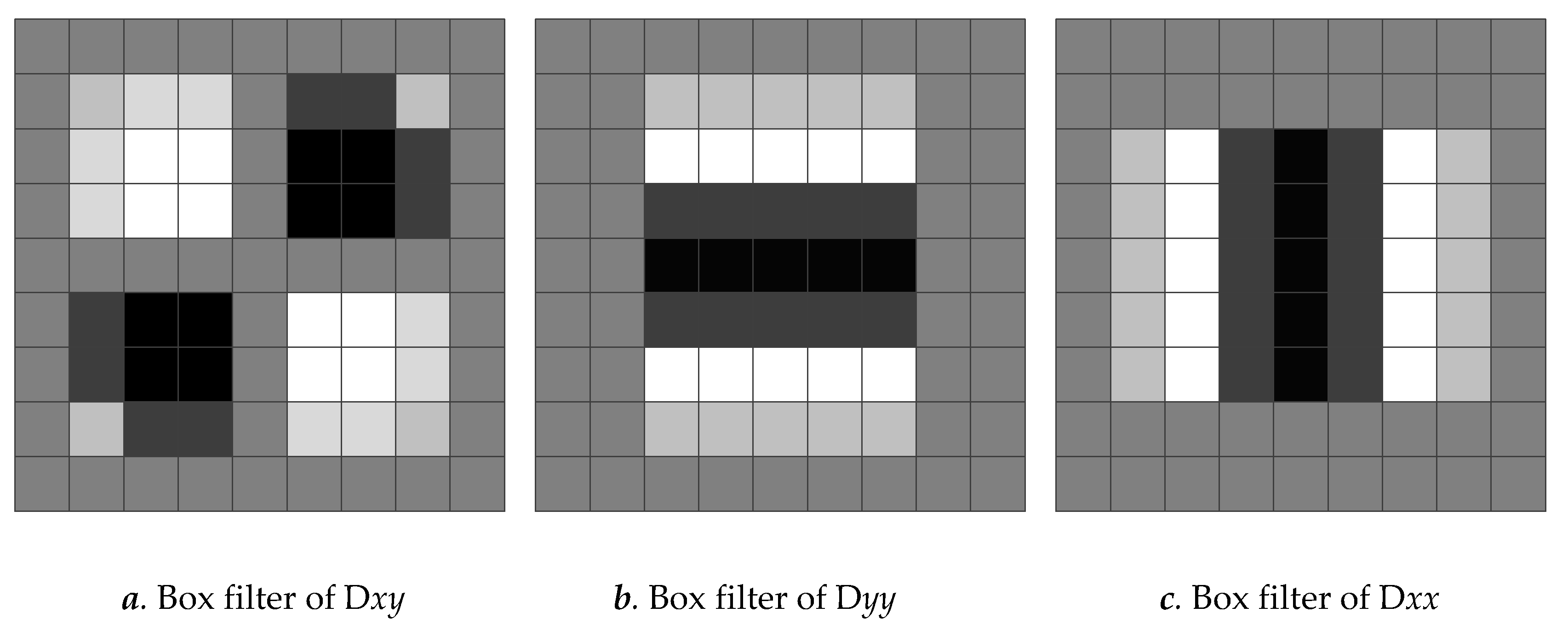
Via the classical SURF, the Hessian matrix is simplified and approximated by box filters and used to segment the second-order Gaussian template. Each filter has three values: 1 (white), 0 (grey), and −1 (black). The white area and black area of the filter are usually approximated by the white/light white regions and black/light black regions. In this way, the computing speed is accelerated at the cost of accuracy. The problem can be solved by the improved SURF, in which each box filter has five values: 1, 0.5, 0, −0.5, and −1. As shown in Figure 4 below, the proportion of regional areas in the improved filters is increased.
To extract the texture features from the target images, a new matrix was established whose size is the same as that of the original image. The positions of SURF feature points were colored black, while those of the other points were colored white in the matrix. The original image can be generated based on the new matrix. The weight of the greyscale matrix of the original image was 0.7, while that of the new matrix was 0.3. The two weights were added up to form the greyscale matrix of the updated image:
M ^ I m a g e = 0.7 M I m a g e + 0.3 M S u r f
where M ^ I m a g e and M I m a g e are the greyscale matrices of the updated and original images, respectively; M S u r f is the black–white matrix of SURF feature points.

3.2. Feature Matching

In this paper, the cloud model method is modified by grey correlation degree for case matching.

3.2.1. Cloud Model Method

The cloud model can depict fuzzy and random samples with expectation Ex, entropy En, and super entropy He. Let η i ( t ) be the multidimensional features extracted from each image, where i = 1, …, n. Then, the generation algorithm of a normal cloud model can be explained as follows.
The expectation, entropy, and super entropy of a sample can be expressed as:
E x [ η i ( t ) ] = 1 i η i ( t )
E n ( η i ( t ) ) = 1 i { η i ( t ) E x [ η i ( t ) ] } 2
H e [ η i ( t ) ] = 0.1
On this basis, normal random numbers η ^ i ( t ) can be generated taking E x [ η i ( t ) ] and E n [ η i ( t ) ] as expectation and standard deviation, respectively, and normal random numbers E n [ η i ( t ) ] can be generated taking E n [ η i ( t ) ] and H e [ η i ( t ) ] as expectation and standard deviation, respectively. Then, the certainty degree can be calculated as:
μ ( t ) = exp [ i [ ( η i ( t ) E x [ η i ( t ) ] 2 2 E n [ η i ( t ) ] 2 ] ]
The certainty degree of the next image frame can be obtained similarly through the above steps. Comparing the certainty degree μ ( t ) of each image frame, the η i ( t ) with the smallest certainty degree was determined as the coordinates of the target.

3.2.2. Modification of Cloud Model Method

The cloud model method was modified via grey correlation analysis through the following steps. Suppose the case library has m cases and n eigenvalues. Then, the impact degree matrix F can be established as:
F = [ f 11 f 12 f 1 n f 21 f 22 f 2 n f m 1 f m 2 f m n ] = f ( i j ) m × n ,     i = 1 , ...... , n ,     j = 1 , ...... , m
where fij is the impact degree from the i-th source case and the j-th index f i j ( 0 , 1 ) . Each row of matrix F stands for a source case, while each column represents an eigenvalue.
The correlation between each index can be measured by:
ξ i j = 1 - k | E x ( t ) j f i j | | E x ( t ) j f i j | + k | E x ( t ) j f i j |
where k is a resolution coefficient, k ( 0 , 1 ) . The value of k is usually set to 0.5. The judgement matrix of grey correlation degree F’ can be expressed as:
F = [ ξ 11 ξ 12 ξ 1 n ξ 21 ξ 22 ξ 1 n ξ m 1 ξ m 2 ξ m n ] = ξ ( i j ) m × n ,   ξ i j ( 0.66 , 1 )
Once a new case was found to match a source case, the eigenvalue of that case was modified. Since the grey correlation degree is constantly changing between two cases in matrix F’, the eigenvalue of the matched case keeps changing. The normalized form of matrix F’ can be described as:
w i j = ( ξ i j 0.66 ) / j = 1 6 ( ξ i j 0.66 )      i = ( 1 , 2 m )    ,          j = ( 1 , 2 , 3 , 4 , 5 , 6 )

4. Experiments

The data on cargo A of enterprise W over 15 months were selected for the experimental verification of the proposed approach. The data were counted separately in the three sales channels. The target supply chain involves 1734 manufacturers, suppliers, distributors, and retailers. One minute was taken as the minimum statistical unit, the data of a day were viewed as a case, the cases of a year were adopted as a training sample, and the cases of three months were considered as a test sample. The state of inventory is measured by change rate, change quantity, and total amount. The feedback information is change quantity and total amount. The objectives of the optimal control were minimal time and minimal energy, which correspond to minimal time and minimal cost in supply chain management.

4.1. Comparison between Different Feedback Devices

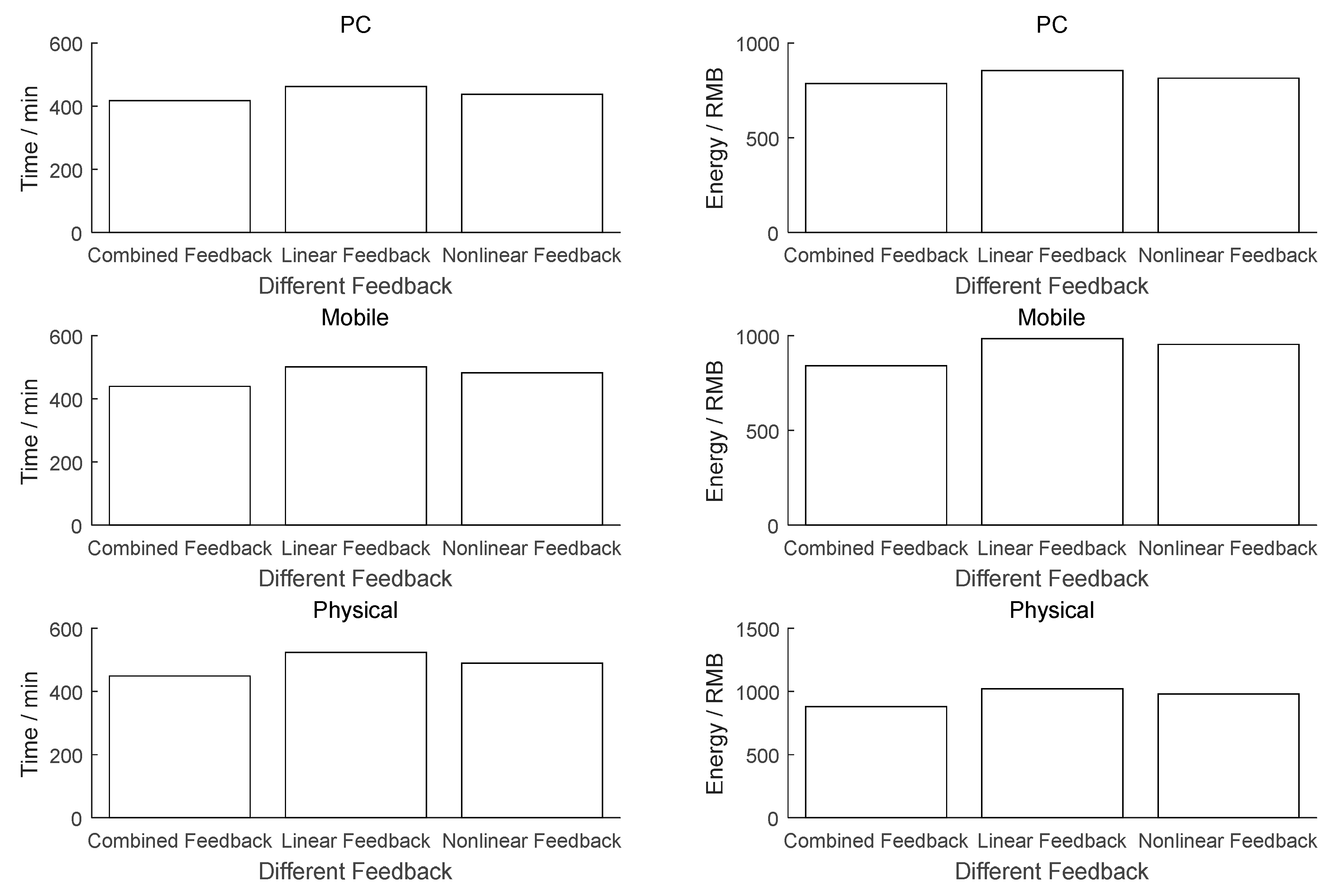
The effect of the combined feedback device, which includes both linear and nonlinear feedbacks, was contrasted with that of a linear feedback device and that of a nonlinear feedback device. The comparison results of one case are shown in Table 1.
As shown in Table 1, the combined feedback device achieved the minimal time and cost among the three devices: It consumed 8% less time than the linear feedback device and 8% less time than the nonlinear one; it cost 10% less money than the linear feedback device and 5% less money than the nonlinear one.
The three devices were further compared with the data of three months. The results of each month and the mean results of the three months are both illustrated in Figure 5 below. It can be seen that the combined feedback device outperformed the linear one by 12% and the nonlinear one by 8% in time consumption and outshined the linear one by 10% and the nonlinear one by 10% in cost. In other words, the combined feedback device achieved the best results among the three devices.
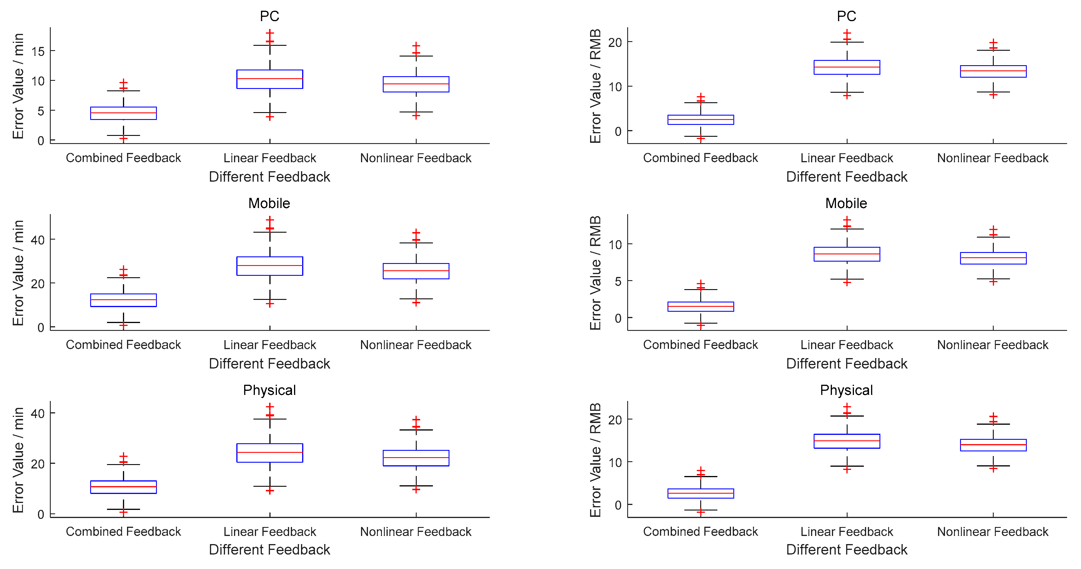
Figure 6 shows the gap between the actual results and the expected results of the test sample obtained by each device. It is clear that the combined feedback device generated a smaller error and median error than the other two devices.
The excellent performance of the combined feedback device is attributable to its comprehensive consideration of both linear and nonlinear factors, which are present in the state of each node in actual supply chains.

4.2. Comparison between Different Solutions to the Optimal Control Curve

The variational method was compared with the shooting method, multiple shooting method, DMOC method, and Gauss pseudospectral method through experiments on the solution of the optimal control curve. The optimal control results of a case are listed in Table 2 below.
As shown in Table 2, the variational method was less efficient than the contrastive methods, as evidenced by the 5-second lag. However, this method outperformed the other methods in accuracy.
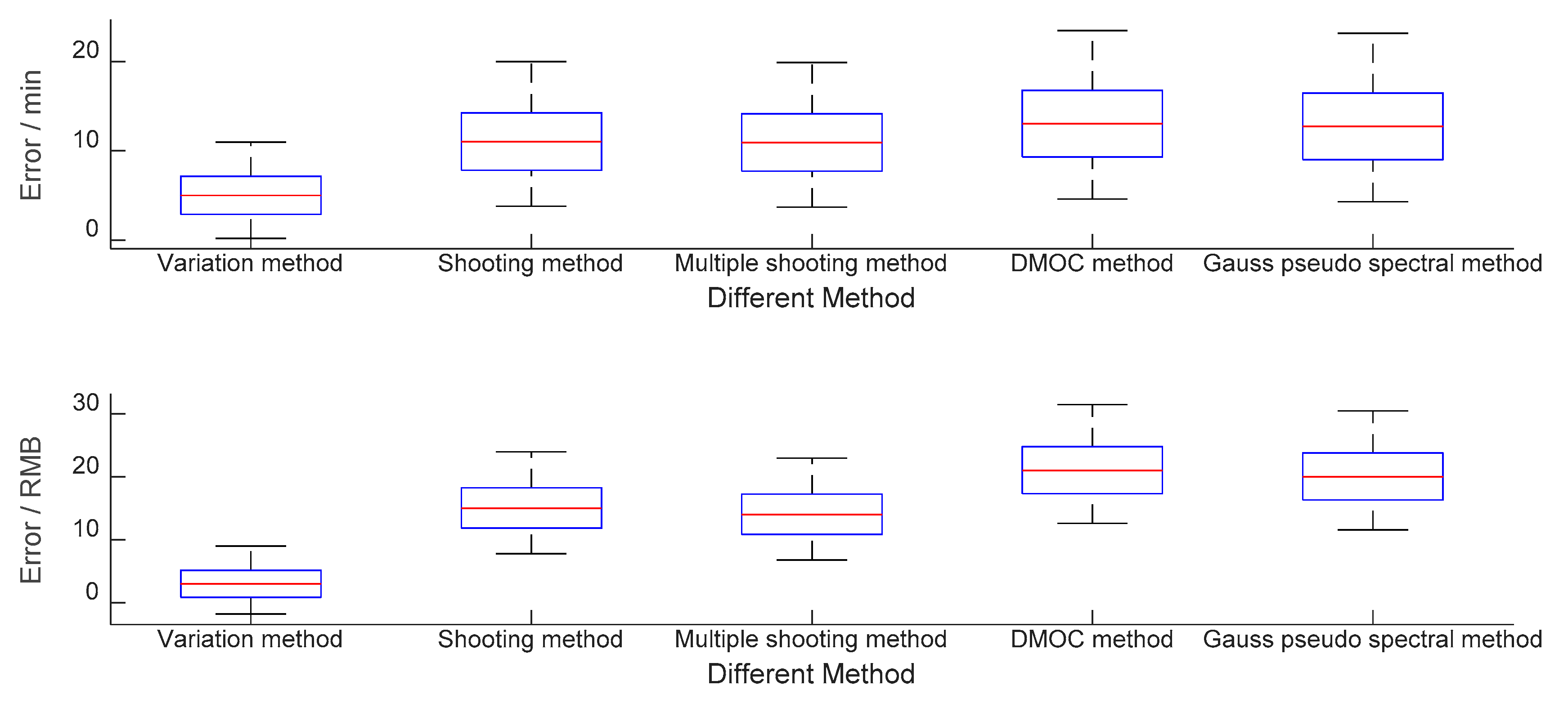
The error between the results and the expected values of each method was obtained and plotted in Figure 7. It is clear that the variational method generated a smaller error and median error than the other methods.
The good performance of the variation method results from its basis: the solution of continuous function. By contrast, the other methods, based on discrete functions, only obtain approximate solutions. The slight lag in efficiency is offset by the exceptionally good accuracy of the variational method.

4.3. Comparison between Different Image Formats

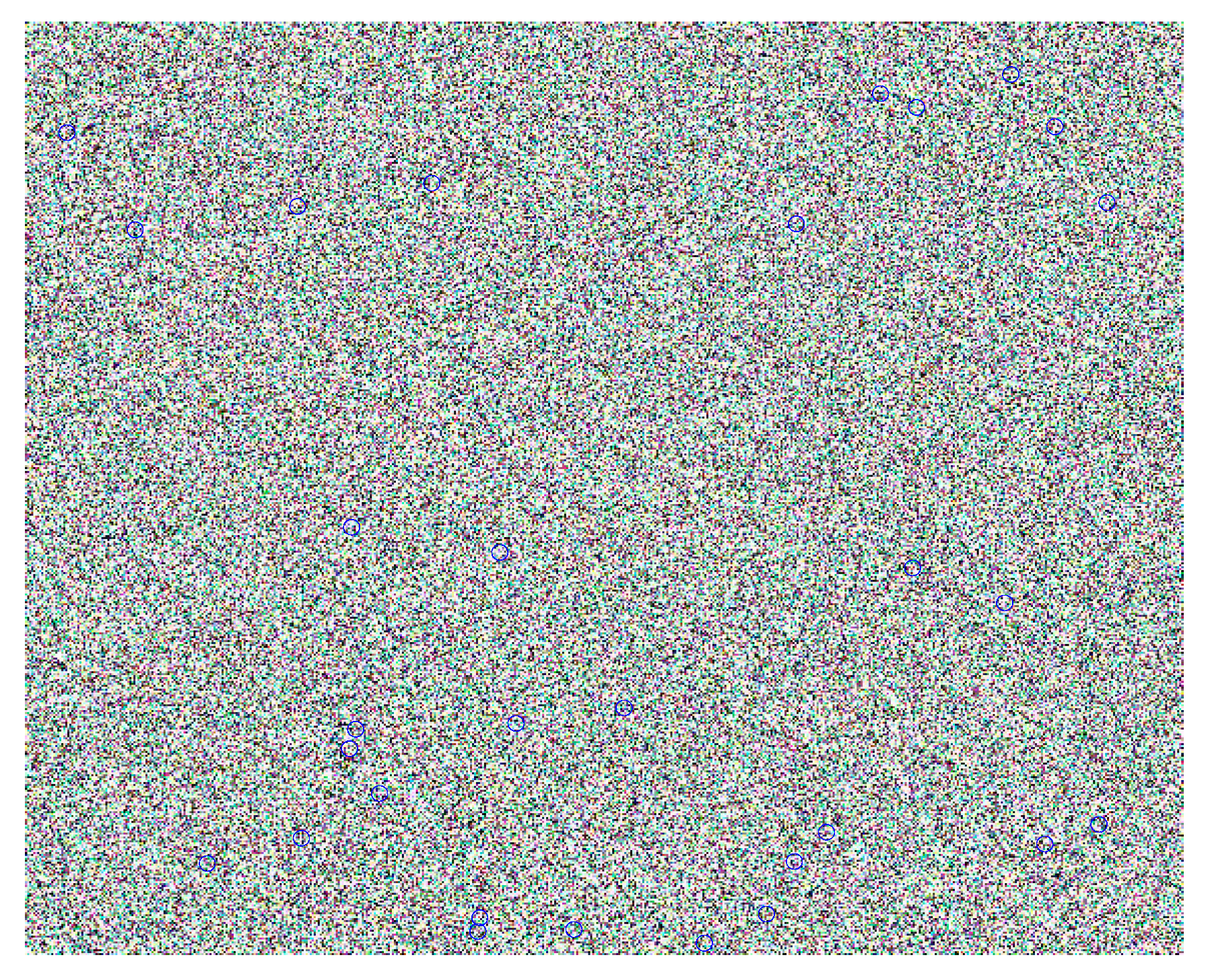
During the research, the information of the supply chain was saved as images. One of the images is shown in Figure 8. For comparison, the image modified according to SURF feature points is presented in Figure 9.
Obviously, Figure 9 is much clearer than Figure 8. The clearer the image, the more accurate the information is. Thus, SURF modification does contribute to the information retention.
The hard disk space of the proposed format was compared with .rar, a common format of compressed images. According to the results in Table 3, the proposed format only occupied 0.5% of the hard disk space, much smaller than that (50%) of the .rar format.
The good result of the proposed format can be explained as follows. To save hard disk space, each double precision floating-point number was transformed into an integer, a data unit into a point, and three data tables into a color image.

4.4. Comparison with Single Feature Extraction Methods

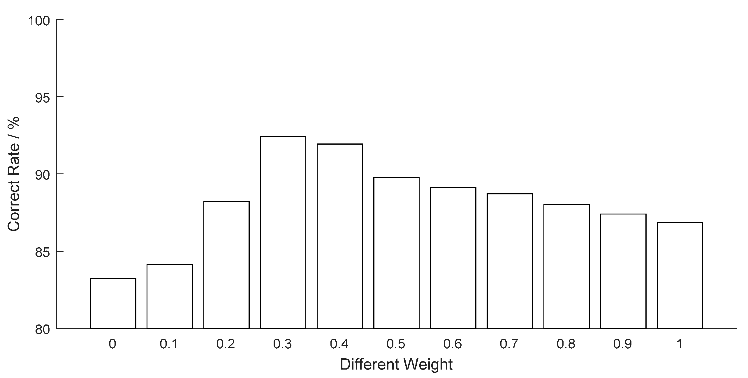
A total of 2160 test samples and different weights were adopted to compare the proposed SURF-GoogLeNet with SURF and GoogLeNet. The correctly matched cases of each method are shown in Table 4 below, and the relationship between correct rate and weight is illustrated in Figure 10.
From Table 4, it can be seen that the proposed method achieved an 8.8% higher correct rate than SURF and a 5.09% higher correct rate than GoogLeNet. Figure 10 shows that the correct rate peaked at the weight of 0.3, the same as that in Equation (20). Thus, 0.3 is the optimal weight for case matching.
The proposed SURF-GoogLeNet performed better than the other methods, because it combines the traditional image processing method and deep learning method. The former is good at extracting intrinsic features, while the latter does well in the extraction of texture features.

4.5. Comparison with Hybrid Feature Extraction Methods

SURF-GoogLeNet was further compared with several hybrid feature extraction methods, including detection free tracking (DFT), incremental visual tracking (IVT), compression tracking (CT) and deep learning tracking (DLT). The results on 2160 test samples are recorded in Table 5 below.
As shown in Table 5, the proposed method had an edge over the other hybrid feature extraction methods. On correct rate, SURF-GoogLeNet was 1.29% higher than the DLT method, 2.4% higher than the CT method, 3.47% higher than the IVT method, and 2.87% higher than the DFT method.

4.6. Comparison between Case Matching Methods

The grey-cloud method was compared with the grey method, the k-nearest neighbor (KNN) method, the BP method and the cloud method, all of which are well-received case matching strategies. The results on 2160 test samples are displayed in Table 6 below.
As can be seen from Table 6, the grey-cloud method realized a higher correct rate than any of the contrastive method: It is 1.71% more accurate than the KNN, 1.89% more accurate than the grey method, 1.15% more accurate than the cloud method, and 1.25% more accurate than the BP method.
The advantage of the grey-cloud method in case matching arises from the combination of the cloud model, whose uncertainty improves the matching robustness, and the grey correlation analysis, which can accurately identify the objective weight of each index.

5. Discussion and Conclusions

In pursuit of the optimal logistics control in the OSC, this paper designed the combined feedback device and adopted the variational method to control the logistics in a single node, saved the information of the supply chain as images to save hard disk space, combined the SURF and deep learning methods into a hybrid feature extraction approach, and selected the grey-cloud method for case matching. The effectiveness of the proposed methods was verified through experiments. The research findings shed new light on the management of supply chains.
There is some linear feedback information in logistics allocation. If the commodity is a daily consumable, the logistics feedback information basically meets the linear rule. There is also some nonlinear feedback information in logistics allocation. If the goods are production materials, the feedback information of logistics may meet the nonlinear rule. Therefore, this study has certain practical significance. However, there are still some limitations to this research. With the development of a supply chain, there might be more than three sales channels in the future, which cannot be analogized simply as the red, green and blue (RGB) in images. At the same time, if the omnichannel supply chain has more data dimensions, the variational method may have the result of no solution or infinite solution. Further, the proposed methods still consume a long time due to the adjustment of the case library. In future, parallel computation should be considered to speed up the operation.

Author Contributions

All authors contributed to the present paper with the same effort in finding available literature resources, as well as writing the paper.

Funding

This research is supported by Beijing Science and Technology Plan Project with No. Z191100001419001, Beijing Municipal Natural Science Foundation with No. 4192042, National Science Fund subsidized project with No. 61627816.

Acknowledgments

The authors would like to thank the anonymous reviewers for their constructive comments.

Conflicts of Interest

The authors declare no conflict of interest.

References

  1. Xue, H.; Lin, Y. The omni-channel consumer segmentation method based on consumption data stream mining. In Proceedings of the 2017 IEEE 2nd International Conference on Big Data Analysis (ICBDA), Beijing, China, 10–12 March 2017. [Google Scholar]
  2. Du, S.; Wang, L.; Hu, L. Omnichannel management with consumer disappointment aversion. Int. J. Prod. Econ. 2019, 215, 84–101. [Google Scholar] [CrossRef]
  3. Gupta, V.K.; Ting, Q.; Tiwari, M.K. Multi-period price optimization problem for omnichannel retailers accounting for customer heterogeneity. Int. J. Prod. Econ. 2019, 212, 155–167. [Google Scholar] [CrossRef]
  4. Xue, H.; Yuan, Y.; Lin, Y.; Cai, J. Early warning decision-making system based on cloud computing technology for retail supply chain unconventional emergency. In Proceedings of the 2017 IEEE 2nd International Conference on Cloud Computing and Big Data Analysis (ICCCBDA), Chengdu, China, 28–30 April 2017. [Google Scholar]
  5. Xue, H.; Cai, J.; Yuan, Y.; Lin, Y. The collaborative decision of profit distribution in retail supply chain under emergency. In Proceedings of the 2017 29th Chinese Control and Decision Conference (CCDC), Chongqing, China, 28–30 May 2017. [Google Scholar]
  6. Alfares, H.K.; Attia, A.M. A supply chain model with vendor-managed inventory, consignment, and quality inspection errors. Int. J. Prod. Res. 2017, 55, 5706–5727. [Google Scholar] [CrossRef]
  7. Sarkar, M.; Hur, S.; Sarkar, B. Effects of Variable Production Rate and Time-Dependent Holding Cost for Complementary Products in Supply Chain Model. Math. Probl. Eng. 2017, 2017, 1–13. [Google Scholar] [CrossRef]
  8. White, A.S.; Censlive, M. Control system analysis of labour supply flows in production systems. J. Manuf. Syst. 2015, 37, 316–327. [Google Scholar] [CrossRef]
  9. Chang, J.S.; Chang, C.; Shi, M. A market-based martingale valuation approach to optimum inventory control in a doubly stochastic jump-diffusion economy. J. Oper. Res. Soc. 2015, 66, 405–420. [Google Scholar] [CrossRef]
  10. Sadeghi, J.; Mousavi, S.M.; Niaki, S.T.A.; Sadeghi, S. Optimizing a bi-objective inventory model of a three-echelon supply chain using a tuned hybrid bat algorithm. Transp. Res. Part E: Logist. Transp. Rev. 2014, 70, 274–292. [Google Scholar] [CrossRef]
  11. Pedrosa, A.D.M.; Näslund, D.; Jasmand, C. Logistics case study based research: towards higher quality. Int. J. Phys. Distrib. Logist. Manag. 2012, 42, 275–295. [Google Scholar] [CrossRef]
  12. Zhao, K.; Yu, X. A case based reasoning approach on supplier selection in petroleum enterprises. Expert Syst. Appl. 2011, 38, 6839–6847. [Google Scholar] [CrossRef]
  13. Germani, M.; Mandolini, M.; Mengoni, M.; Peruzzini, M. Platform to support dynamic collaborative design processes in virtual enterprises. Int. J. Comput. Integr. Manuf. 2013, 26, 1003–1020. [Google Scholar] [CrossRef]
  14. Poon, T.; Choy, K.L.T.; Chow, H.K.; Lau, H.C.; Chan, F.T.; Ho, K. A RFID case-based logistics resource management system for managing order-picking operations in warehouses. Expert Syst. Appl. 2009, 36, 8277–8301. [Google Scholar] [CrossRef]
  15. Lao, S.; Choy, K.L.T.; Ho, G.; Tsim, Y.; Poon, T.; Cheng, C. A real-time food safety management system for receiving operations in distribution centers. Expert Syst. Appl. 2012, 39, 2532–2548. [Google Scholar] [CrossRef]
  16. Lam, H.; Choy, K.L.T.; Ho, G.; Kwong, C.; Lee, C. A real-time risk control and monitoring system for incident handling in wine storage. Expert Syst. Appl. 2013, 40, 3665–3678. [Google Scholar] [CrossRef]
  17. Choy, K.L.; Chow, K.H.; Moon, K.L.; Zeng, X.; Lau, H.C.; Chan, F.T.; Ho, G.T. A RFID-case-based sample management system for fashion product development. Eng. Appl. Artif. Intell. 2009, 22, 882–896. [Google Scholar] [CrossRef]
  18. Lim, S.F.W.; Srai, J.S. Examining the anatomy of last-mile distribution in e-commerce omnichannel retailing: A supply network configuration approach. Int. J. Oper. Prod. Manag. 2018, 38, 1735–1764. [Google Scholar] [CrossRef]
  19. Schank, R.C. Dynamic Memory: A Theory of Reminding and Learning in Computers and People; Cambridge University Press: New York, NY, USA, 1983. [Google Scholar]
  20. Martinez, A.J.P.; Stapleton, O.; Van Wassenhove, L.N. Field vehicle fleet management in humanitarian operations: A case-based approach. J. Oper. Manag. 2011, 29, 404–421. [Google Scholar] [CrossRef]
  21. Wang, X.F.; Zhu, W.D. Design and Stability Analysis of an Integral Time-Delay Feedback Control Combined with an Open-Loop Control for an Infinitely Variable Transmission System. J. Dyn. Syst. Meas. Control 2018, 140, 011007. [Google Scholar] [CrossRef]
  22. Sun, G.; Ma, P.; Ren, J.; Zhang, A.; Jia, X. A stability constrained adaptive alpha for gravitational search algorithm. Knowl.-Based Syst. 2018, 139, 200–213. [Google Scholar] [CrossRef]
  23. Ebadollahi, S.; Saki, S. Wind turbine torque oscillation reduction using soft switching multiple model predictive control based on the gap metric and kalman filter estimator. IEEE Trans. Ind. Electron. 2017, 65, 3890–3898. [Google Scholar] [CrossRef]
  24. Bitew, W.T.; Grabovsky, Y. Higher regularity of uniform local minimizers in Calculus of Variations. Proc. Am. Math. Soc. 2017, 145, 5215–5222. [Google Scholar] [CrossRef] [Green Version]
  25. March, R.; Riey, G. Analysis of a variational model for motion compensated inpainting. Inverse Probl. Imaging 2017, 11, 997–1025. [Google Scholar] [CrossRef]
  26. Bélaise, C.; Dal Maso, F.; Michaud, B.; Mombaur, K.; Begon, M. An EMG-marker tracking optimisation method for estimating muscle forces. Multibody Syst. Dyn. 2018, 42, 119–143. [Google Scholar] [CrossRef]
  27. Blonigan, P.J.; Wang, Q. Multiple shooting shadowing for sensitivity analysis of chaotic dynamical systems. J. Comput. Phys. 2018, 354, 447–475. [Google Scholar] [CrossRef] [Green Version]
  28. Moore, A.; Ober-Blöbaum, S.; Marsden, J.E. Trajectory Design Combining Invariant Manifolds with Discrete Mechanics and Optimal Control. J. Guid. Control. Dyn. 2012, 35, 1507–1525. [Google Scholar] [CrossRef] [Green Version]
  29. Shareef, Z.; Trächtler, A. Simultaneous path planning and trajectory optimization for robotic manipulators using discrete mechanics and optimal control. Robotica 2016, 34, 1322–1334. [Google Scholar] [CrossRef]
  30. Zaky, M.; Machado, J.T.; Zaky, M. On the formulation and numerical simulation of distributed-order fractional optimal control problems. Commun. Nonlinear Sci. Numer. Simul. 2017, 52, 177–189. [Google Scholar] [CrossRef]
  31. Williams, T.; Taroyan, Y. Formation of a Dense Flux Rope by a Siphon Flow. Astrophys. J. 2018, 852, 77. [Google Scholar] [CrossRef]
  32. Chen, R.; Imani, F.; Reutzel, E.; Yang, H. From Design Complexity to Build Quality in Additive Manufacturing—A Sensor-Based Perspective. IEEE Sens. Lett. 2018, 3, 1–4. [Google Scholar] [CrossRef]
  33. Kan, C.; Chen, R.; Yang, H. Image-guided Quality Control of Biomanufacturing Process. Procedia CIRP 2017, 65, 168–174. [Google Scholar] [CrossRef]
  34. Imani, F.; Cheng, C.; Chen, R.; Yang, H. Nested gaussian process modeling for high-dimensional data imputation in healthcare systems. In Proceedings of the 2018 Institute of Industrial and Systems Engineers Annual Conference and Expo, IISE, Orlando, FL, USA, 19–22 May 2018. [Google Scholar]
  35. Imani, F.; Chen, R.; Diewald, E.; Reutzel, E.; Yang, H. Image-guided Variant Shape Analysis of Layerwise Build Quality in Additive Manufacturing. In Proceedings of the International Manufacturing Science and Engineering Conference, ASME, Erie, PA, USA, 10–14 June 2019. [Google Scholar]
  36. Scott, G.J.; England, M.R.; Starms, W.A.; Marcum, R.A.; Davis, C.H. Training Deep Convolutional Neural Networks for Land-Cover Classification of High-Resolution Imagery. IEEE Geosci. Remote Sens. Lett. 2017, 14, 549–553. [Google Scholar] [CrossRef]
  37. Zhao, G.; Ahonen, T.; Matas, J.; Pietikainen, M. Rotation-Invariant Image and Video Description with Local Binary Pattern Features. IEEE Trans. Image Process. 2011, 21, 1465–1477. [Google Scholar] [CrossRef] [PubMed]
  38. Zhao, X.; Dawson, D.; Sarasua, W.A.; Birchfield, S.T. Automated traffic surveillance system with aerial camera arrays imagery: Macroscopic data collection with vehicle tracking. J. Comput. Civ. Eng. 2016, 31, 04016072. [Google Scholar] [CrossRef]
  39. Hu, Y.; Li, L. 3D reconstruction of end-effector in autonomous positioning process using depth imaging device. Math. Probl. Eng. 2016, 2016, 8972764. [Google Scholar] [CrossRef]
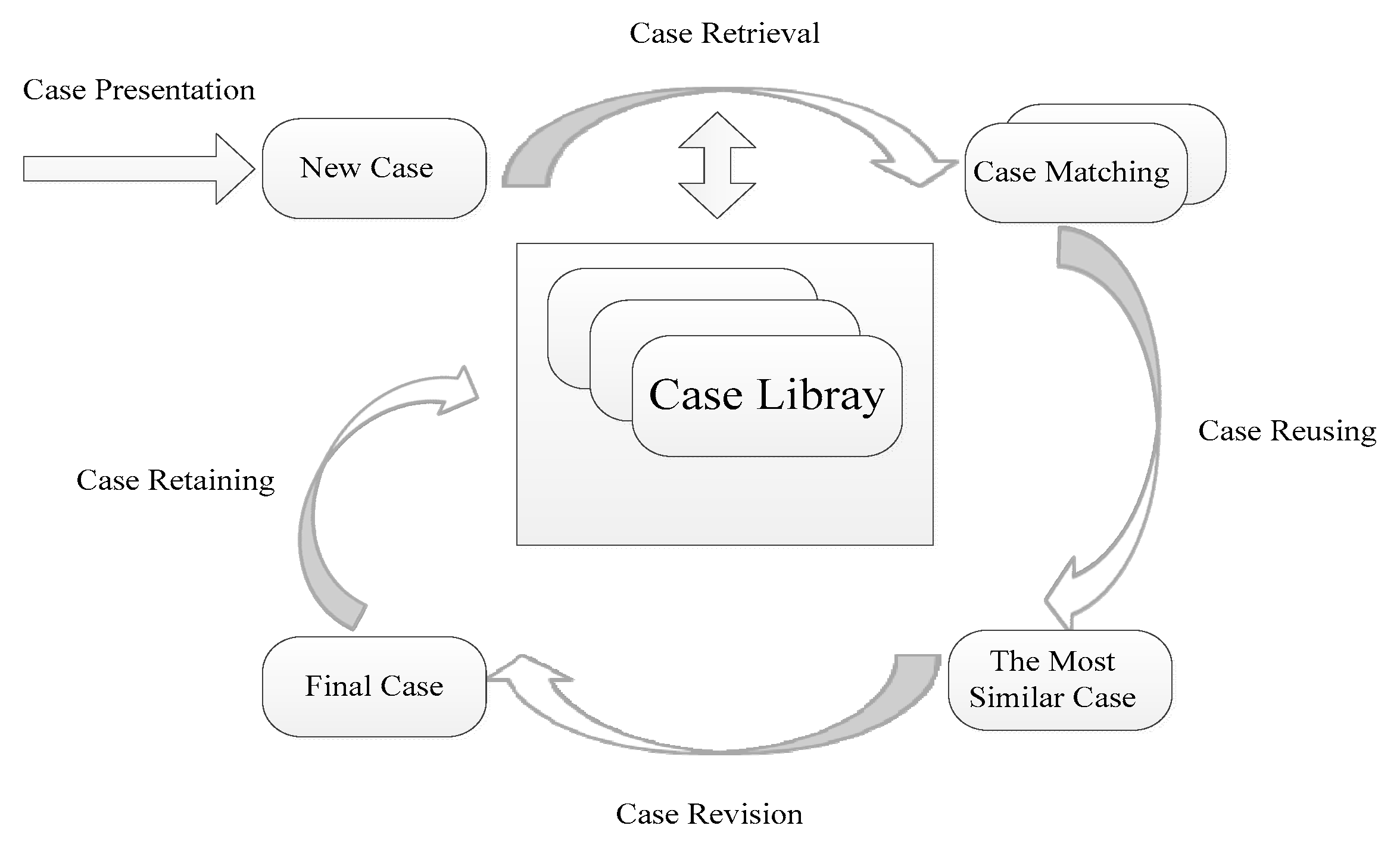
Figure 1. The flowchart of case-based reasoning (CBR).
Sustainability 11 06014 g001
Figure 2. The block diagram of the combined feedback device.
Sustainability 11 06014 g002
Figure 3. Structure of GoogLeNet.
Sustainability 11 06014 g003
Figure 4. Improved box filter.
Sustainability 11 06014 g004
Figure 5. Results on three-month data.
Sustainability 11 06014 g005
Figure 6. The errors of the three devices.
Sustainability 11 06014 g006
Figure 7. The errors of the five methods.
Sustainability 11 06014 g007
Figure 8. An original image.
Sustainability 11 06014 g008
Figure 9. SURF-modified image.
Sustainability 11 06014 g009
Figure 10. Relationship between correct rate and weight.
Sustainability 11 06014 g010
Table 1. Comparison of three feedback devices.
No.NamePCMobilePhysical
Time
(min)
Energy
(¥)
Time
(min)
Energy
(¥)
Time
(min)
Energy
(¥)
1Combined feedback417.6786.12439.4841.62449.1879.14
2Linear feedback462.5854.69501.2984.26523.71021.36
3Nonlinear feedback437.8814.97482.3953.67489.4979.41
Table 2. Comparison of optimal control results.
No.NameOperation Time (s)Time (min)Energy (¥)
1Variational method30.2423.6833.66
2Shooting method22.3429.6845.68
3Multiple shooting method23.5428.9844.72
4DMOC method24.6432.1851.17
5Gauss pseudo spectral method25.1431.9850.34
Table 3. Hard disk space of images in different formats.
No.Data FormatData DurationFile Size.Rar Compress
1.mat10s604MB312 MB
2.csv10s451MB229 MB
3.xlsx10s367MB190 MB
4.jpg10s16.6KB8.9 KB
Table 4. Correct rates of the three methods.
No.NameSurfGoogLeNetSurf–GoogLeNet
1correct number179818761986
2correct rate83.24%86.85%91.94%
Table 5. Results of different hybrid feature extraction methods.
No.NameDFTIVTCTDLTSurf–GoogLeNet
1correct number19241911193419581986
2correct rate89.07%88.47%89.54%90.6591.94%
Table 6. Results of different case matching methods.
No.NameGray-CloudKNNGrayCloudBP
1correct number19861949194519611959
2correct rate91.94%90.23%90.05%90.79%90.69%