Abstract
Catchment runoff is significantly affected by climate condition changes. Predicting the runoff and analyzing its variations under future climates play a vital role in water security, water resource management, and the sustainable development of the catchment. In traditional hydrological modeling, fixed model parameters are usually used to transfer the global climate models (GCMs) to runoff, while the hydrologic model parameters may be time-varying. It is more appropriate to use the time-variant parameter for runoff modeling. This is achieved by incorporating the time-variant parameter approach into a two-parameter water balance model (TWBM) through the construction of time-variant parameter functions based on the identified catchment climate indicators. Using the Ganjiang Basin with an outlet of the Dongbei Hydrological Station as the study area, we developed time-variant parameter scenarios of the TWBM model and selected the best-performed parameter functions to predict future runoff and analyze its variations under the climate model projection of the BCC-CSM1.1(m). To synthetically assess the model performance improvements using the time-variant parameter approach, an index Δ was developed by combining the Nash–Sutcliffe efficiency, the volume error, the Box–Cox transformed root-mean-square error, and the Kling–Gupta efficiency with equivalent weight. The results show that the TWBM model with time-variant C (evapotranspiration parameter) and SC (water storage capacity of catchment), where growing and non-growing seasons are considered for C, outperformed the model with constant parameters with a Δ value of approximately 5% and 10% for the calibration and validation periods, respectively. The mean annual values of runoff predictions under the four representative concentration pathways (RCPs) exhibited a decreasing trend over the future three decades (2021–2050) when compared to the runoff simulations in the baseline period (1982–2011), where the values were about −9.9%, −19.5%, −16.6%, and −11.4% for the RCP2.6, RCP4.5, RCP6.0, and RCP8.5, respectively. The decreasing trend of future precipitation exerts impacts on runoff decline. Generally, the mean monthly changes of runoff predictions showed a decreasing trend from January to August for almost all of the RCPs, while an increasing trend existed from September to November, along with fluctuations among different RCPs. This study can provide beneficial references to comprehensively understand the impacts of climate change on runoff prediction and thus improve the regional strategy for future water resource management.
1. Introduction
Climate changes like global warming are presently occurring due to continued emissions of greenhouse gases. The changes in the climate system will significantly affect climate variables such as precipitation and temperature. According to the Fifth Assessment Report (AR5) of the Intergovernmental Panel on Climate Change (IPCC) [1], the projected precipitation and temperature show great changes and exhibit heterogeneity in different regions. For example, increases of precipitation and temperature occur in high-latitude regions of the Northern Hemisphere; global surface temperature change for the end of 21st century is expected to exceed 1.5 °C for most of the representative concentration pathways (RCPs) [2]. The changes and variability of climate conditions can significantly affect catchment hydrological cycles, leading to changes in regional water resources [3]. Therefore, it is of great importance to evaluate catchment runoff variations under the future climate projections.
To obtain future climate datasets, global climate models (GCMs) forced with various projected greenhouse gas and aerosol emissions have been developed to generate information about historical and future climate conditions. The GCMs are based on mathematical representations of ocean, sea-ice, land, and atmospheric processes that play crucial roles in Earth’s climate system [2]. As one of the GCMs, the BCC-CSM1.1(m) was developed based on the BCC-CSM1.1 by the Beijing Climate Center (BCC), China Meteorological Administration (CMA). The major difference between the two versions is the model resolution in the atmospheric component. The two versions of the GCM from the BCC have been widely applied in China due to its favorable feasibility and good performance [4,5,6,7,8,9]. For instance, Ding et al. [10] used the BCC-CSM1.1(m) to produce the model inputs for the simulation of future irrigation water requirements. Sridhar et al. [11] employed the BCC-CSM1.1 to reproduce precipitation for trend analysis.
The prediction of catchment runoff is usually conducted based on hydrological models, where the forcing inputs and model parameters are required and play significant roles in runoff modeling. The BCC-CSM1.1(m) described above can provide the model input data under different climate scenarios in the future period, while for model parameters, the traditional way is to use the calibrated parameter values to predict runoff by assuming the model parameters to be stationary. These are regarded as constants in hydrological modeling. However, it is no longer appropriate to use constant parameters, especially for hydrological modeling under the changing environment. A temporal variability of the model parameters exists due to the influence of catchment condition changes including climate condition and catchment characteristics (e.g., land use and land cover) [12,13,14,15,16]. For example, Wang and Tang [17] found that rainfall and vegetation were the dominant controlling factors on the parameter of a Budyko equation, which is derived for mean annual water balance and is independent of temporal scale. Wallner and Haberlandt [18] found that the storage coefficient of the HBV-IWW model, which is a modified version of the HBV model and was developed by the Swedish Meteorological and Hydrological Institute (SMHI) [19], has a close relationship with potential evaporation. Zhang et al. [20] quantified the impact of vegetation change on the landscape parameter of a Budyko equation, and found that the parameter was sensitive to changes in catchment vegetation conditions.
Three optional approaches are mainly applicable to obtain the time-variant model parameters. The first is to calibrate parameters in consecutive subsets of the historical data and attempts to obtain their values separately in each period using optimization algorithms [20,21]. The second method is to estimate model parameters via data assimilation techniques based on the available observations [12,15]. Another method of estimating time-variant parameters is to establish the parameter functions as dependent on covariates that can reflect the variability of catchment conditions [22]. To our knowledge, this approach is the most suitable way to model with time-variant parameters. Fortunately, studies have been described regarding the time-variant parameter method. Westra et al. [16] defined the maximum capacity of the production store (one parameter of a lumped rainfall–runoff model GR4J) as a combined function of covariates including an annual sinusoid of time step t, the previous 365 day rainfall and potential evapotranspiration, and a linear function of time step t. Recently, Deng et al. [23] proposed a time-variant parameter approach for monthly hydrological models. In this method, indicators of catchment properties are identified and then used as independent variables of model parameter functions. Brief descriptions about the procedures are introduced in Section 2.3. The advantage of this method is that the time-variant parameter can be estimated directly based on the established parameter functions, where the covariates are available in future climate projections.
A limited number of studies have focused on runoff prediction under future climates by considering the time-variant parameter in monthly hydrological models. Constant model parameters calibrated based on the historical data have limited extrapolative ability and may weaken the model credibility in runoff estimations. The constructed parameter functions are dependent on catchment indicators, which can directly incorporate the variations of catchment conditions into the estimation of model parameters. Thus, considering the time-variant parameter is essential for more reliable and accurate runoff prediction under climate changing scenarios.
The objective of this study was to predict the catchment runoff under future climate change scenarios using the time-variant parameter approach for a monthly hydrological model, and to analyze the variation trend and amplitude of the water resources in the study area. The rest of this paper is structured as follows. Section 2 describes the study area and datasets, along with the approaches used to construct the time-variant parameter function and predict the runoff. The results and discussions are presented in Section 3, followed by a summary in Section 4.
2. Materials and Methods
2.1. Study Area and Data Sources
2.1.1. Study Area
With a controlling area of about 80,948 km2, the Ganjiang Basin is the seventh largest tributary of the Yangtze River. It is located in the middle and lower reaches of the Yangtze River and mainly lies in Jiangxi Province, China. The land use and land cover in the Ganjiang Basin has been affected significantly by the tree and grass plantations and reservoir construction. For example, the total storage capacity of the large reservoir, which has a total storage of greater than 1.0 × 10⁸ m3, was approximately 3.0 × 10⁹ m3 during the period of 1980–2006 [24]. These implements led to an increase in the water holding capacity of the catchment, which potentially results in the temporal variation of hydrological model parameter(s) related to the catchment storage capacity. The land use types of the Ganjiang Basin include woodland, cropland, grassland, water body, and built-up land, while the woodland is the main type.
The basin outlet of the study area is the Dongbei Hydrological Station, and the drainage area is about 40,231 km2. For simplicity, the basin selected for study is referred to as GJDB, as shown in Figure 1. The GJDB lies in the subtropical region with a humid climate and sufficient rainfall characterized by a climate aridity index (i.e., ratio of mean annual potential evapotranspiration to mean annual precipitation) of about 0.74. Due to the influence of typhoons and monsoon, precipitation across the GJDB is mainly concentrated in March to June (rainy season), which accounts for about 54% of annual precipitation. The mean annual precipitation of the GJDB from 1982 to 2011 was approximately 1700 mm. The mean annual potential evapotranspiration is about 1251 mm, and the multi-year runoff coefficient is 0.49.
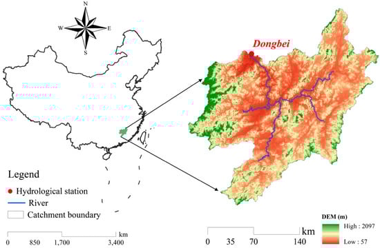
Figure 1.
A brief description of the study area.
2.1.2. Observed Datasets
Daily meteorological data including precipitation (P), potential evapotranspiration (PET), temperature (Tm), and monthly runoff (Q) for the period of 1980–2011 were used in this study. The potential evapotranspiration was estimated using the temperature-based Hargreaves method (HM) [25,26] based on meteorological data from the China Meteorological Data Sharing Service System. The runoff records of Dongbei Station were obtained from the local Hydrological Bureau. Monthly P and PET were calculated as the sum of the corresponding daily data. Mean areal P and PET were calculated by averaging the monthly P and PET from the available meteorological stations in and around the GJDB. The datasets from 1980 to 2006 were used for the exploratory analysis including parameter estimation and the construction of time-variant parameter functions. Note that the first two years (1980–1981) were reserved for model warm-up. The period 2007–2011 was used for validation (i.e., time-variant parameter scenario selection and model evaluation). After the construction of the time-variant parameter functions and model performance evaluation, datasets over the three decades (1982–2011) were used as the baseline to compare to the corresponding results from the future climate projection. The data from the global climate model are introduced in the next section.
2.1.3. Data from the Global Climate Model (GCM)
The future climate datasets were obtained from the BCC-CSM1.1(m), participating in the CMIP5 experiment [27]. The BCC-CSM1.1(m) was developed based on the Beijing Climate Center Climate System Model version 1.1 with an approximate atmospheric resolution of 1.125°. This model was selected since it can fully meet the data requirement to force the monthly hydrological model used in this study. Moreover, it has been widely applied for climate impact studies with favorable feasibility in China [10,28]. Monthly precipitation and maximum and minimum temperatures under four emissions scenarios over the 2021–2050 period were processed to generate the model inputs. Emissions scenarios includes four representative concentration pathways (RCPs): RCP2.6, RCP4.5, RCP6.0, and RCP8.5. Among the four RCPs, RCP2.6 represents a low radiative forcing emission (2.6 W/m2 by 2100), RCP4.5 and RCP6.0 are two intermediate scenarios (4.5 W/m2 and 6.0 W/m2 by 2100, respectively), while RCP8.5 exhibits the highest level of radiative forcing (8.5 W/m2 by 2100). The monthly potential evapotranspiration PET was estimated by using the Hargreaves method (HM) [25,26], since less data are required and it outperforms the Penman–Monteith (PM) method under a certain degree of inaccuracy in meteorological observations [29]. The daily maximum and minimum temperatures were used to calculate the PET via the HM method, then the daily PET was transformed into monthly values. To avoid the systematic bias brought by the coarse spatial resolution and the GCM model, a downscaling method named quantile mapping [30,31] was employed to adjust the GCM output and transfer them from a coarse grid to a points scale using a transfer function between the model outputs and observations. The details on this approach can be found in Wang et al. [32].
The downscaled monthly precipitation and processed monthly potential evapotranspiration were used as model inputs for future runoff predicting. The forcing inputs and runoff predictions over the future three decades were then analyzed and compared to those in the baseline period.
2.2. Hydrological Model
A two-parameter monthly water balance model (TWBM) [33] was used for runoff simulation in this study. The TWBM model has been widely used in hydrological simulation and prediction since it performs very well and is easy to use [12,34,35]. Two major modules are contained in this model including the actual evapotranspiration and runoff. The TWBM model has only two parameters (i.e., the evapotranspiration parameter C and water storage capacity SC), and one state variable (i.e., the soil moisture content S). First, the monthly actual evapotranspiration is computed by:
where Pt, Et, and PETt are the monthly precipitation, monthly actual evapotranspiration, and monthly potential evapotranspiration, respectively. C is the first parameter related to evapotranspiration. The runoff at current month Qt is dependent on the soil water content and is calculated based on the equation . The available water for runoff at the beginning of given month is calculated by , after loss through actual evapotranspiration Et, with St−1 being the soil water moisture at the end of the previous month and at the beginning of current month. Then, Qt is computed by the following equation:
where SC is the second parameter that represents the water storage capacity of catchment. Finally, the soil water content at the end of given month St is updated according to the water conservation law:
2.3. Time-Variant Parameter Method
A recently proposed time-variant parameter approach [23] was applied for runoff simulation under a changing environment (e.g., catchment climatic conditions). The key steps of this method are: (1) model parameters are estimated by the ensemble Kalman filter (EnKF) based on the datasets of calibration period; (2) time-variant covariates are identified and selected to build the functional forms of model parameters; and (3) a model with constructed parameter functions is used for runoff simulation in different climate change scenarios. It should be noted that the time-variant covariates used for parameter function construction usually include catchment climatic indicators and catchment properties (e.g., land use and land cover). The catchment climate indicators and the leaf area index are incorporated into the parameter functions since they are available in the future climate projections, thereby the time-variant parameter forecasts can be calculated directly. Here, we only provide a brief description of this approach, and details could be found in Deng et al. [23].
2.3.1. Estimation of Model Parameter Series
The EnKF is used to simultaneously estimate the state variable and parameters of the TWBM model in the calibration period. The assimilation procedure is given in Appendix A. The data assimilation setup plays an important role in the estimation of time-variant parameters. Its impacts on the data assimilation results have been explored in many studies [36,37,38,39]. In this study, the ensemble size and error terms in input and output were set following the previous [12,23,40,41]. The number of ensemble members was set to 1000 for the study case. The standard deviations of the error terms including model state variable, parameters, and runoff observation were determined with the most accurate runoff simulation as the criterion [12]. These were proportional to the magnitude of the corresponding values. The proportional factors were 1% for model parameters (i.e., C and SC); 5% for the state variable (i.e., S); and 10% for monthly runoff, Q.
2.3.2. Construction of Parameter Functional Forms
The two parameters were allowed to vary temporally and were assumed to be a function of the identified catchment indicators. The evapotranspiration parameter C directly affects the calculation of the actual evapotranspiration. The precipitation P and temperature Tm have correlations with this procedure, the functional form of C was thus assumed to be a linear function with independent variables of P and Tm. Furthermore, a proxy for vegetation (i.e., the leaf area index (LAI)) was selected to construct the time-variant functions of C since vegetation conditions have been reported to be strongly related to evapotranspiration [20,42]. The changes of catchment water storage capacity SC are usually a long-term process (e.g., several years or decades) that have a close relationship to the catchment properties. Thus, the antecedent monthly precipitation and potential evapotranspiration were used as potential independent variables of its functions. The time-lag between the climatic indicators and temporal variation of parameter C was considered since the evaporation process at the current time might be related to the climate conditions at a previous time. Therefore, catchment indicators including LAI, P(t), P(t−1), Tm(t), and Tm(t−1) were used for correlation analysis with the estimates of parameter C; while 1-, 3-, 6-month antecedent monthly precipitation and potential evapotranspiration (P1, P3, P6, PET1, PET3, PET6) were for parameter SC [23,43].
The Spearman rank correlation coefficient (rs) was employed to evaluate the relationship between the parameter estimates and catchment indicators, since their correlations are not necessarily linear [21]. It ranges from −1 to 1, and a value of −1 represents a completely negative correlation; while 1 represents a completely positive correlation, and zero means no correlation for pairwise data series. It should be noted that the mean monthly values of the catchment indicators and parameter estimates were calculated for correlation analysis, aiming to eliminate the impact of the slight fluctuations in parameter estimates on the correlation analysis.
Linear and quadratic functional forms were applied for the construction of the model parameter function based on the previous literature by Deng et al. [23]. Specifically, two types of functional forms including the univariate quadratic function with an independent variable of LAI and multivariate linear function with independent variable of P and Tm were implemented to build the functions of parameter C. Furthermore, the growing season (May to October) and non-growing season (November to April) were considered to precisely reflect the seasonal variability of the catchment vegetation conditions. For parameter SC, the multivariate linear functional form was used to construct its time-variant functions. The general functional forms are as follows:
where a, b, and d are the parameters of the time-variant parameter functions; P and Tm are the identified precipitation and temperature with time-step being considered for parameter C; AP and AEP are the identified antecedent monthly precipitation and potential evapotranspiration for parameter SC.
The function parameters a, b, and d were estimated using the nonlinear and multiple linear regression method based on the series of identified catchment factor and assimilated parameter estimates. Furthermore, results from the model with constant parameters were used for a comparison with those from the time-variant parameter cases. The shuffled complex evolution (SCE-UA) algorithm proposed by Duan et al. [44] was applied for the calibration of constant parameters.
2.4. Model Performance Evaluation
Four hydrologically oriented model diagnostics (i.e., the Nash–Sutcliffe efficiency (NSE) [45], the volume error (VE), the Box–Cox transformed root-mean-square error (TRMSE) [46], and the Kling–Gupta efficiency (KGE) [47]) were used to assess the model performance in monthly runoff estimation. Note that the TRMSE and KGE were focused primarily in low and high flows, respectively.
where Qsim,t and Qobs,t are the simulated and observed monthly runoff for the tth month, respectively; is the mean values of the runoff observations; and are the transformed runoff simulations and observations for the tth month; represents the Box–Cox transformation of Q, γ = 0.3, as recommended by Misirli et al. [48]; r is the Pearson’s linear correlation coefficient; α and β are the ratios of standard deviations and means between simulated and observed runoff, respectively; and n denotes the total number of months.
The NSE ranges from to 1 and has been widely applied for the assessment of goodness-of-fit for hydrological simulations to observations. A NSE value of 1 represents a perfect match of runoff simulations to observations, and a value of 0 indicates that the model simulations are equivalent to the mean value of the observations. The VE is a measure of the total volume bias between the simulated and observed runoff. For example, the water balance requirement is fully satisfied when VE equals zero. The positive and negative values indicate the model underestimation and overestimation, respectively. The smaller the value of TRMSE, the better the runoff performance in low flows. The KGE ranges from to 1, and a KGE value of 1 means a perfect fit in high flows.
To synthesize the evaluation in different aspects of runoff performances, an index combined the four performance criteria with equivalent weight was proposed to assess the improvements of model performance using the time-variant parameter approach. A positive Δ value indicates that the constructed time-variant parameter functions could yield improvement in model performance; while the model with constant parameters outperformed the model with time-variant parameters if the Δ value is negative.
where Δ denotes the improvements achieved by the model with time-variant parameters; and subscript tv and tc represent the model with time-variant parameters and constant parameters, respectively.
3. Results and Discussions
3.1. Functions of Time-Variant Parameters
The independent variables used for establishing the functional forms of two model parameters were selected based on the results of the Spearman rank correlation coefficient rs. Specifically, the indicator with the biggest |rs| value in precipitation P indicators and temperature indicators Tm was used as the independent variable for parameter C; while the indicator with the biggest |rs| value in antecedent precipitation and antecedent potential evapotranspiration indicators was used as the independent variable for parameter SC. Table 1 presents the identified catchment indicators and time-variant parameter scenarios for parameters C and SC. As shown in Table 1, the functional forms with identified catchment factors for parameter C were the quadratic function of LAI and linear function of P(t) and Tm(t). For parameter SC, the function case was the linear function of P6 and PET3. Scenarios of both time-variant C and SC were conducted by combining the single time-variant parameter case. In total, nine time-variant parameter scenarios were implemented in monthly runoff modeling including four scenarios for parameter C, one scenario for parameter SC, and four scenarios for their combinations. Note that the other parameter value was set as the calibrated constant value when a single parameter is time-variant.

Table 1.
Description of the parameter scenarios and their functional forms with identified catchment indicators for parameters C and SC in the GJDB.
The model performance improvement index was computed and presented in Figure 2 for the calibration and validation periods. The results show that scenario C3 + SC1 (the red rectangular line in Figure 2) gave the highest Δ values among all of the parameter scenarios, suggesting that runoff performance improvement can be achieved when parameters C and SC are treated as time-variant, especially when parameter C is built using the multivariate linear function with the growing and non-growing seasons being considered. As shown in Figure 3, the errors of the runoff simulations and observations were compared between the scenarios of C3 + SC1 and the constant parameters. At the yearly scale, the mean absolute relative errors of the runoff simulations were 7.69% and 7.74% for the time-variant and constant scenarios in the calibration period, respectively; while they were 8.39% and 8.66% in the validation period, respectively. The results in Figure 3a demonstrate that the simulated annual runoff from the time-variant parameter model was generally closer to the observed runoff, even though the errors in part of the years were larger than those from the constant parameter model. For the mean monthly runoff in the entire period of 1982–2011 (Figure 3b), results from the parameter scenario of C3 + SC1 showed smaller relative errors than those from the constant parameter case for almost each month, except for January and November, where the former case had slightly bigger or the same relative errors when compared with the latter. The best-performed parameter functions are listed below:
where Cg(t) and Cng(t) are parameter C in the growing season and non-growing season, respectively; P(t) and Tm(t) are the monthly precipitation and monthly mean temperature at the tth month; P6(t) and PET3(t) are the 6-month antecedent monthly precipitation and 3-month antecedent monthly potential evapotranspiration at the tth month, respectively; and symbol ‘e’ in the empirical equations represents the power of ten in scientific notation.
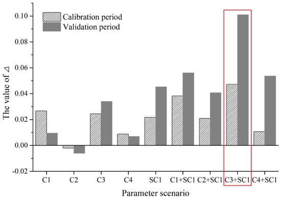
Figure 2.
Model performance improvement index Δ in different time-variant parameter scenarios during the calibration period (1982–2006) and validation period (2007–2011).
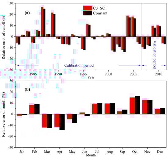
Figure 3.
Relative errors between the simulated runoff from the TWBM model with the best-performed time-variant parameters and constant parameters and runoff observation. (a) Annual values during the calibration period (1982–2006) and validation period (2007–2011). (b) Mean monthly values in the period of 1982–2011.
The time-variant parameter instead of constant parameters offers a possibility for hydrological models to adapt to potential changes of catchment conditions, although the traditional statistical tests did not seem to be very much improved. The constructed time-variant parameter functions in Equation (12) were applied for predicting runoff of the GJDB under the different RCPs in future climate projection (i.e., the BCC-CSM1.1(m)). Thus, the changes of runoff volume under the future climate projection could be analyzed based on the runoff predictions estimated by the model with the time-variant parameters. The corresponding results are presented in the following section.
3.2. Runoff Predictions under Future Climate Scenarios
According to the time-variant parameter functions built above, the model parameters of the TWBM model were calculated using the climatic data obtained from the four different RCPs in the BCC-CSM1.1(m). The monthly runoff in the future period of 2021–2050 was then estimated and the results are shown in Table 2 and Figure 4. Table 2 first presents the mean annual statistics of precipitation, potential evapotranspiration, and runoff for the historical and future periods, respectively. The mean annual precipitation for all four RCPs showed a decreasing trend when compared to the historical records of 1982–2011, with different degrees from −8.9% to −13.5%. The mean annual potential evapotranspiration showed an increased trend for RCP4.5, RCP 6.0, and RCP8.5 with relative differences from 3.5% to 6.2%, while it decreased to 1.9% for RCP2.6 when compared to the in the historical period. The mean annual runoff in the future period was smaller than that in the historical period for all four RCPs. It should be noted that the value for the historical period was computed based on the monthly estimations from the TWBM model under the best-performed parameter scenario (C3 + SC1); the value computed based on the observations is also provided in the bracket, which was very close to the model estimates. Therefore, the from the model simulations was used for consistency in both the historical and future periods. The climate conditions of the GJDB behaved more arid under the future climate projection, with a larger aridity index, but still belonged to the humid climate. The decreasing runoff could generally be explained by the decreasing precipitation and increasing potential evapotranspiration, according to the water balance law at the mean annual scale.
Table 2.
Comparison of hydrological characteristics in the historical and future periods. The mean annual precipitation and potential evapotranspiration were calculated directly based on the historical records and future climatic data from the four different RCPs in the BCC-CSM1.1(m) projection. The mean annual runoff was calculated based on the runoff estimates from the TWBM model with the best-performed time-variant parameters. The numbers in the brackets of the historical data row are the observations or value computed based on the observations.
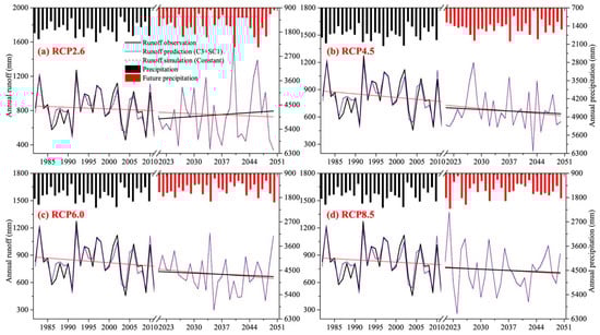
Figure 4.
Comparison of yearly runoff simulations (1982–2011) and predictions (2021–2050) estimated by the best-performed time-variant parameter (C3 + SC1) model and constant parameter model under the four RCPs of the BCC-CSM1.1(m): (a) RCP2.6, (b) RCP4.5, (c) RCP6.0, (d) RCP8.5. The runoff observations in the historical period are also presented in these plots. The precipitation observations (black solid bars) and predictions (red solid bars) are also present. Note that the red and black straight lines are the linear trend of the simulated runoff of the entire historical and future periods, and runoff prediction in the future period, respectively.
Figure 4 shows the observed runoff and runoff predictions estimated by the TWBM model under the C3 + SC1 parameter scenario at the yearly time scale, along with the runoff simulations from the constant parameter scenario. The yearly simulated runoff matched the runoff observations very well in the historical period. The linear trends for the runoff series were also analyzed with the trend lines being presented in the subplots. The simulated runoff series in both the periods of 1982–2011 and 2021–2050 were combined first for trend analysis, and the results showed that they had a decreased trend with different slopes. The results demonstrate that the runoff volumes in the GJDB will decrease under the four RCPs in the future climate projection. The precipitation decline exerts a dominant influence upon runoff decline in the GJDB. The runoff predictions in the period of 2021–2050 also behaved as a decreasing trend under the scenarios of RCP4.5, RCP6.0, and RCP 8.5, whilst under the scenario of RCP2.6, they had an increasing trend. Table 3 gives the linear trend lines of the observed runoff and simulated runoff for different periods under each RCP scenario. The rank of the linear trend slopes for the four RCPs was RCP4.5 < RCP6.0 < RCP8.5 < RCP2.6, sorted in the increasing order over the entire historical and future periods for the runoff predictions, which matched the ranks of ΔP and ΔQ (shown in Table 2) very well. Generally, the runoff volumes under the four RCPs will decrease in the future climate projection along with precipitation decline.
Table 3.
Linear trend lines of the simulated and observed runoff in the historical period, simulated runoff for both historical and future periods, and runoff prediction under the future climate projection. The simulated runoff was estimated by the TWBM model under the best-performed time-variant parameter scenario (C3 + SC1).
Figure 5 presents the predicted monthly runoff series from the time-variant and constant parameter scenarios in the future period (2021–2050), respectively. Results show that the main difference in the runoff predictions for the time-variant and constant parameter scenarios was the values in high and low flows. Generally, runoff predictions from the time-variant parameter scenario have bigger values in high flows than those from the constant parameter scenario; while in low flows, runoff predictions from the former scenario usually have restively smaller values than those from the later scenario. At the yearly scale, the annual runoff predictions between the two parameter scenarios (Figure 4) showed no significant differences. This might partially be explained by the equalization of runoff values from a monthly time scale to an annual scale. Furthermore, the relatively small improvement achieved by the time-variant parameter model will also produce relatively close runoff results to the constant parameter model. However, it is still meaningful to consider the temporal variability of the model parameter that may occur, caused by the significant changes of catchment conditions [23].
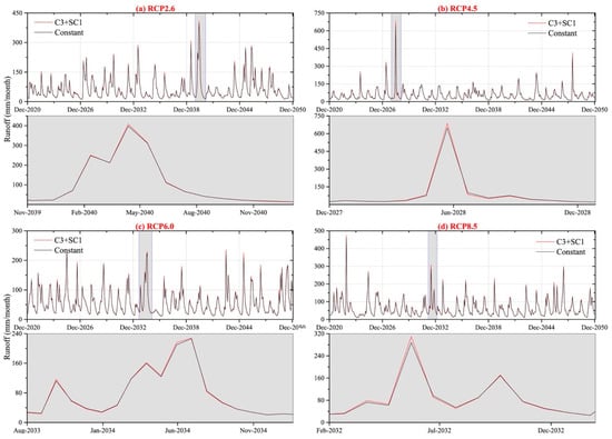
Figure 5.
Comparison of monthly runoff predictions obtained from the best-performed time-variant parameter (C3 + SC1) model and constant parameter model under the four RCPs of the BCC-CSM1.1(m): (a) RCP2.6, (b) RCP4.5, (c) RCP6.0, (d) RCP8.5. The subplots with colored shadow are the zoomed lines of the runoff series from the entire future period (2021–2050).
Figure 6 presents the relative changes of precipitation and runoff predictions between the future period and the baseline period at the mean monthly scale. The mean monthly changes of runoff predictions and precipitation are presented in Figure 7 for all four RCPs. Generally, the results in both figures show that the mean monthly precipitation increased monotonically from January to June, and decreased monotonically from June to December in the period of 1982–2011. Results show that the mean monthly precipitations under the different RCPs still had the same seasonal pattern to the mean monthly precipitation in the historical period, except that the values in RCP2.6 showed a second peak in September, besides June. The mean monthly runoff prediction varied along with the mean monthly precipitation in each RCP scenario. In the future climate, the mean monthly values of predicted runoff will mostly be smaller than those of runoff simulations in the current climate, while bigger values will exist for a few months in part of the RCP scenarios. For example, mean monthly runoff values from September to November in RCP2.6 and RCP8.5 and from October to November in RCP6.0 had a significantly larger value than those in the historical period. The results demonstrate that the precipitation decline exerts a dominant impact upon runoff decline in the GJDB under future climate conditions.
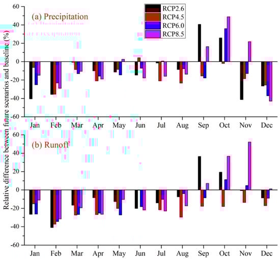
Figure 6.
Relative differences of mean monthly precipitation and runoff between the four RCPs under the future climate scenario (2021–2050) and baseline period (1982–2011). The runoff predictions in the future period and runoff simulations in the baseline period were obtained from the TWBM model with the best-performed time-variant parameter (C3 + SC1).

Figure 7.
Mean monthly runoff simulations during the historical period (1982–2011) and mean monthly runoff predictions under the four RCPs of the BCC-CSM1.1(m) estimated by the best-performed time-variant parameter (C3 + SC1) model, along with the corresponding precipitation observation and predictions from the RCPs.
For the GJDB, the runoff predicted by the TWBM model with constructed time-variant parameter functions will decrease in mean annual values under the four RCPs from the future climate projection of the BCC-CSM1.1(m). The seasonal patterns of precipitation and runoff predictions had no significant changes compared to those in the baseline period (1982–2011), while changes in volumes and fluctuations occur for the two hydrological variables. According to the predicted results above, the decreasing of water volume in GJDB may increase the pressure from the water supply (e.g., December to May of the next year) in the future to a certain extent. Measurements such as reservoir operation, water conservation, and sustainable utilization of water resources might provide potential ways to relieve the contradiction between the water supply and demand.
4. Summary
This study focused on the runoff prediction and its change analysis in the GJDB for the future periods of 2021–2050. To predict the runoff under a climate projection of the BCC-CSM1.1(m), the time-variant parameter approach was incorporated into a two-parameter monthly water balance model (TWBM) by constructing the time-variant parameter functions, where the model parameters can be calculated based on the future climate indicators, thereby predicting the future monthly runoff under the climate model projection. The runoff predictions under the four representative concentration pathways (RCPs) were then analyzed and compared to the simulated runoff in the historical period (1982–2011). Conclusions can be drawn as follows:
(1) The time-variant parameter method for the TWBM model improved the runoff performance in the catchment hydrograph, water volume bias, and low and high flows. Compared to the traditional constant parameter method, the synthetical improvement index Δ under the best-performed parameter scenario reached 5% and 10% for the calibration and validation periods, respectively. For the GJDB, parameter C of the TWBM model can be made dependent on the climate factors of P(t) and Tm(t) using a linear function with the growing and non-growing seasons being considered, while parameter SC can be represented as a multivariate linear function of P6 and PET3.
(2) Under the four RCP scenarios in the BCC-CSM1.1(m) projection, the mean annual changes of runoff in the GJDB will be about −9.9%, −19.5%, −16.6%, and −11.4% for the RCP2.6, RCP4.5, RCP6.0, and RCP8.5, respectively. The runoff decline can mainly be explained by the decreasing precipitation. The mean monthly runoff will decrease from January to August for the four RCPs (except for RCP4.5 in June), while significant increases exist from September to November, especially for RCP2.6 and RCP8.5. Both the precipitation and runoff patterns in the future period are generally consistent with the historical period.
When using the forcing data obtained from the climate projection for runoff prediction for a future climate, uncertainty from the global climate models might affect the model parameter calculation and model inputs, thereby leading to uncertainty in the runoff modeling results. In this study, future climatic datasets from only one climate projection were applied for runoff prediction in the GJDB. In the next work, future climatic data should be based on an ensemble of different global climate models (GCMs) to consider the uncertainty of the GCMs. Furthermore, exploring the influence of the parameter function uncertainty would be a meaningful topic for runoff modeling.
Author Contributions
Conceptualization, C.D. and W.W.; Methodology, C.D.; Software, C.D.; Validation, C.D. and W.W.; Formal analysis, W.W.; Investigation, C.D.; Resources, C.D.; Data curation, C.D.; Writing—original draft preparation, C.D.; Writing—review and editing, C.D. and W.W.; Visualization, W.W.; Supervision, W.W.; Project administration, C.D. and W.W.; Funding acquisition, C.D. and W.W.
Funding
This study was supported by the National Natural Science Foundation of China (51809071, 51779073), the Distinguished Young Fund Project of Jiangsu Natural Science Foundation (BK20180021), the Fundamental Research Funds for the Central Universities (2018B55314) and the China Postdoctoral Science Foundation (2017M621613).
Acknowledgments
We thank the China Meteorological Data Sharing Service System for providing part of the data used in this study (http://data.cma.cn/). The authors would like to thank the editor and the anonymous reviewers for their comments that helped improve the quality of this paper.
Conflicts of Interest
The authors declare no conflict of interest.
Appendix A. Ensemble Kalman Filter
The state equation in the EnKF is described by:
where xt+1 is the state vector at time t + 1; θ is the system parameter vector; f represents the forecasting model operator (e.g., monthly hydrological model); ut+1 represents the inputs for the hydrological model (e.g., precipitation and potential evapotranspiration); and εt represents the model error term, which follows a Gaussian distribution with zero mean and specified covariance Vt.
The observation equation is:
where yt+1 is the observation vector at time t + 1; h is the observation operator that represents the relationship between the observations and states; and ξt+1 is the measurement error, which follows a Gaussian distribution with zero mean and specified covariance Wt+1.
The EnKF assimilation process can then be expressed on the basis of the available state and observation equations:
where is the kth ensemble member forecast at time t + 1; is the kth updated ensemble member at time t; is the kth observation ensemble member generated by adding the error term to the runoff observation; and is the Kalman gain matrix, which represents the weight between the forecasts and observations and can be calculated by:
where is the cross covariance of the forecasted states and forecasted output; is the error covariance of the forecasted output; , where is the ensemble mean of the forecasted members; and N is the ensemble size. The superscript T denotes the matrix transpose.
References
- IPCC. Intergovernmental Panel on Climate Change, 5th Assessment Report: Climate Change 2014; Synthesis Report; World Meteorological Organization: Geneva, Switzerland, 2014. [Google Scholar]
- IPCC. Climate Change 2014: Impacts Adaptation and Vulnerability and Climate Change 2014: Mitigation of Climate Change; Contribution of working group II and working group III to the fifth assessment report of the IPCC; Cambridge University Press: New York, NY, USA, 2014. [Google Scholar]
- Hasan, M.M.; Wyseure, G. Impact of climate change on hydropower generation in Rio Jubones Basin, Ecuador. Water Sci. Eng. 2018, 11, 157–166. [Google Scholar] [CrossRef]
- Sangchul, L.; In-Young, Y.; Sadeghi, A.M.; Mccarty, G.W.; Hively, W.D.; Lang, M.W.; Amir, S. Comparative analyses of hydrological responses of two adjacent watersheds to climate variability and change using the SWAT model. Hydrol. Earth Syst. Sci. 2018, 22, 689–708. [Google Scholar] [CrossRef]
- Xin, X.G.; Wu, T.-W.; Li, J.-L.; Wang, Z.Z.; Li, W.-P.; Wu, F.-H. How well does BCC_CSM1.1 reproduce the 20th century climate change over China? Atmos. Ocean. Sci. Lett. 2013, 6, 21–26. [Google Scholar]
- Zheng, J.; Wang, W.; Cao, X.; Feng, X.; Xing, W.; Ding, Y.; Dong, Q.; Shao, Q. Responses of phosphorus use efficiency to human interference and climate change in the middle and lower reaches of the Yangtze River: Historical simulation and future projections. J. Clean. Prod. 2018, 201, 403–415. [Google Scholar] [CrossRef]
- Chen, L.; Frauenfeld, O.W. Surface air temperature changes over the twentieth and twenty-first centuries in China simulated by 20 CMIP5 models. J. Clim. 2014, 27, 3920–3937. [Google Scholar] [CrossRef]
- Najafi, M.R.; Zwiers, F.W.; Gillett, N.P. Attribution of Observed Streamflow Changes in Key British Columbia Drainage Basins. Geophys. Res. Lett. 2017, 44, 11012–11020. [Google Scholar] [CrossRef]
- Yin, J.; Guo, S.; He, S.; Guo, J.; Hong, X.; Liu, Z. A copula-based analysis of projected climate changes to bivariate flood quantiles. J. Hydrol. 2018, 566, 23–42. [Google Scholar] [CrossRef]
- Ding, Y.; Wang, W.; Song, R.; Shao, Q.; Jiao, X.; Xing, W. Modeling spatial and temporal variability of the impact of climate change on rice irrigation water requirements in the middle and lower reaches of the Yangtze River, China. Agric. Water Manag. 2017, 193, 89–101. [Google Scholar] [CrossRef]
- Sridhar, V.; Modi, P.; Billah, M.M.; Valayamkunnath, P.; Goodall, J.L. Precipitation extremes and flood frequency in a changing climate in southeastern Virginia. J. Am. Water Resour. Assoc. 2019, 55, 780–799. [Google Scholar] [CrossRef]
- Xiong, M.; Liu, P.; Liu, Y.; Cheng, L.; Deng, C.; Gui, Z.; Zhang, X. Identifying time-varying hydrological model parameters to improve simulation efficiency by the ensemble Kalman filter: A joint assimilation of streamflow and actual evapotranspiration. J. Hydrol. 2019, 568, 758–768. [Google Scholar] [CrossRef]
- Pathiraja, S.; Anghileri, D.; Burlando, P.; Sharma, A.; Marshall, L.; Moradkhani, H. Time-varying parameter models for catchments with land use change: The importance of model structure. Hydrol. Earth Syst. Sci. 2018, 22, 2903–2919. [Google Scholar] [CrossRef]
- Deng, C.; Liu, P.; Wang, D.; Wang, W. Temporal variation and scaling of parameters for a monthly hydrologic model. J. Hydrol. 2018, 558, 290–300. [Google Scholar] [CrossRef]
- Meng, S.; Xie, X.; Yu, X. Tracing temporal changes of model parameters in rainfall-runoff modeling via a real-time data assimilation. Water 2016, 8, 19. [Google Scholar] [CrossRef]
- Westra, S.; Thyer, M.; Leonard, M.; Kavetski, D.; Lambert, M. A strategy for diagnosing and interpreting hydrological model nonstationarity. Water Resour. Res. 2014, 50, 5090–5113. [Google Scholar] [CrossRef]
- Wang, D.; Tang, Y. A one-parameter Budyko model for water balance captures emergent behavior in darwinian hydrologic models. Geophys. Res. Lett. 2014, 41, 4569–4577. [Google Scholar] [CrossRef]
- Wallner, M.; Haberlandt, U. Non-stationary hydrological model parameters: A framework based on SOM-B. Hydrol. Process. 2015, 29, 3145–3161. [Google Scholar] [CrossRef]
- SMHI. Integrated Hydrological Modelling System-Manual Version 6.0; Swedish Meteorological and Hydrological Institute: Norrköping, Swden, 2008.
- Zhang, S.; Yang, H.; Yang, D.; Jayawardena, A.W. Quantifying the effect of vegetation change on the regional water balance within the Budyko framework. Geophys. Res. Lett. 2016, 43, 1140–1148. [Google Scholar] [CrossRef]
- Merz, R.; Parajka, J.; Blöschl, G. Time stability of catchment model parameters: Implications for climate impact analyses. Water Resour. Res. 2011, 47, W02531. [Google Scholar] [CrossRef]
- Shao, Q.X.; Traylen, A.; Zhang, L. Nonparametric method for estimating the effects of climatic and catchment characteristics on mean annual evapotranspiration. Water Resour. Res. 2012, 48. [Google Scholar] [CrossRef]
- Deng, C.; Liu, P.; Wang, W.; Shao, Q.; Wang, D. Modelling time-variant parameters of a two-parameter monthly water balance model. J. Hydrol. 2019, 573, 918–936. [Google Scholar] [CrossRef]
- Zhu, J. Study on Runoff Responses to Land Use/Cover Change in Ganjiang Watershed. Master’s Thesis, Jiangxi Normal University, Nanchang, China, 2016. [Google Scholar]
- Hargreaves, G.H. Defining and using reference evapotranspiration. J. Irrig. Drainage Eng. 1994, 120, 1132–1139. [Google Scholar] [CrossRef]
- Droogers, P.; Allen, R.G. Estimating reference evapotranspiration under inaccurate data conditions. Irrig. Drain. Syst. 2002, 16, 33–45. [Google Scholar] [CrossRef]
- Taylor, K.E.; Stouffer, R.J.; Meehl, G.A. An overview of CMIP5 and the experiment design. Bull. Am. Meteorol. Soc. 2012, 93, 485–498. [Google Scholar] [CrossRef]
- Wang, W.; Ding, Y.; Shao, Q.; Xu, J.; Jiao, X.; Luo, Y.; Yu, Z. Bayesian multi-model projection of irrigation requirement and water use efficiency in three typical rice plantation region of China based on CMIP5. Agric. For. Meteorol. 2017, 232, 89–105. [Google Scholar] [CrossRef]
- Wang, W.; Xing, W.; Shao, Q. How large are uncertainties in future projection of reference evapotranspiration through different approaches? J. Hydrol. 2015, 524, 696–700. [Google Scholar] [CrossRef]
- Li, H.B.; Sheffield, J.; Wood, E.F. Bias correction of monthly precipitation and temperature fields from Intergovernmental Panel on Climate Change AR4 models using equidistant quantile matching. J. Geophys. Res. Atmos. 2010, 115. [Google Scholar] [CrossRef]
- Wang, L.; Chen, W. Equiratio cumulative distribution function matching as an improvement to the equidistant approach in bias correction of precipitation. Atmos. Sci. Lett. 2014, 15, 1–6. [Google Scholar] [CrossRef]
- Wang, W.G.; Shao, Q.X.; Yang, T.; Peng, S.Z.; Yu, Z.B.; Taylor, J.; Xing, W.Q.; Zhao, C.P.; Sun, F.C. Changes in daily temperature and precipitation extremes in the Yellow River Basin, China. Stoch. Environ. Res. Risk Assess. 2013, 27, 401–421. [Google Scholar] [CrossRef]
- Xiong, L.; Guo, S.L. A two-parameter monthly water balance model and its application. J. Hydrol. 1999, 216, 111–123. [Google Scholar] [CrossRef]
- Bai, P.; Liu, X.; Liang, K.; Liu, C. Comparison of performance of twelve monthly water balance models in different climatic catchments of China. J. Hydrol. 2015, 529, 1030–1040. [Google Scholar] [CrossRef]
- Wang, W.; Shao, Q.; Yang, T.; Peng, S.; Xing, W.; Sun, F.; Luo, Y. Quantitative assessment of the impact of climate variability and human activities on runoff changes: A case study in four catchments of the Haihe River basin, China. Hydrol. Process. 2013, 27, 1158–1174. [Google Scholar] [CrossRef]
- Wang, D.; Chen, Y.; Cai, X. State and parameter estimation of hydrologic models using the constrained ensemble Kalman filter. Water Resour. Res. 2009, 45, W11416. [Google Scholar] [CrossRef]
- Xie, X.; Zhang, D. A partitioned update scheme for state-parameter estimation of distributed hydrologic models based on the ensemble Kalman filter. Water Resour. Res. 2013, 49, 7350–7365. [Google Scholar] [CrossRef]
- Samuel, J.; Coulibaly, P.; Dumedah, G.; Moradkhani, H. Assessing model state and forecasts variation in hydrologic data assimilation. J. Hydrol. 2014, 513, 127–141. [Google Scholar] [CrossRef]
- Fu, X.L.; Yu, Z.B.; Ding, Y.J.; Tang, Y.; Lü, H.S.; Jiang, X.L.; Ju, Q. Analysis of influence of observation operator on sequential data assimilation through soil temperature simulation with common land model. Water Sci. Eng. 2018, 11, 196–204. [Google Scholar] [CrossRef]
- Deng, C.; Liu, P.; Guo, S.L.; Li, Z.J.; Wang, D.B. Identification of hydrological model parameter variation using ensemble Kalman filter. Hydrol. Earth Syst. Sci. 2016, 20, 4949–4961. [Google Scholar] [CrossRef]
- Xie, X.; Meng, S.; Liang, S.; Yao, Y. Improving streamflow predictions at ungauged locations with real-time updating: Application of an EnKF-based state-parameter estimation strategy. Hydrol. Earth Syst. Sci. 2014, 18, 3923–3936. [Google Scholar] [CrossRef]
- Ye, S.; Li, H.Y.; Li, S.; Leung, L.R.; Demissie, Y.; Ran, Q.H.; Bloschl, G. Vegetation regulation on streamflow intra-annual variability through adaption to climate variations. Geophys. Res. Lett. 2015, 42, 10307–10315. [Google Scholar] [CrossRef]
- Xiong, M.; Liu, P.; Deng, C. Identifying functional form of time-varying hydrological model parameters under changing environment. J. Water Resour. Res. 2018, 7, 351–359. [Google Scholar] [CrossRef]
- Duan, Q.; Gupta, V.K.; Sorooshian, S. Shuffled complex evolution approach for effective and efficient global minimization. J. Optimiz. Theory Appl. 1993, 76, 501–521. [Google Scholar] [CrossRef]
- Nash, J.E.; Sutcliffe, J.V. River flow forecasting through conceptual models part I: A discussion of principles. J. Hydrol. 1970, 10, 282–290. [Google Scholar] [CrossRef]
- Wang, S.; Huang, G.H.; Baetz, B.W.; Cai, X.M.; Ancell, B.C.; Fan, Y.R. Examining dynamic interactions among experimental factors influencing hydrologic data assimilation with the ensemble Kalman filter. J. Hydrol. 2017, 554, 743–757. [Google Scholar] [CrossRef]
- Gupta, H.V.; Kling, H.; Yilmaz, K.K.; Martinez, G.F. Decomposition of the mean squared error and NSE performance criteria: Implications for improving hydrological modelling. J. Hydrol. 2009, 377, 80–91. [Google Scholar] [CrossRef]
- Misirli, F.; Gupta, H.V.; Sorooshian, S.; Thiemann, M. Bayesian recursive estimation of parameter and output uncertainty for watershed models. In Calibration of Watershed Models; American Geophysical Union: Washington, DC, USA, 2013; pp. 113–124. [Google Scholar]


© 2019 by the authors. Licensee MDPI, Basel, Switzerland. This article is an open access article distributed under the terms and conditions of the Creative Commons Attribution (CC BY) license (http://creativecommons.org/licenses/by/4.0/).