Intra-Urban Spatial Disparities in User Satisfaction with Public Transport Services

Abstract

Knowing public transport service’s user satisfaction is essential to maintaining and increasing its quality and demand. Several studies have analysed the factors influencing users’ satisfaction, considering their perceptions of specific attributes of the service. However, other aspects, such as the spatial distribution of users, i.e., their origin neighbourhoods, could significantly affect their satisfaction with the service, showing social inequity patterns. This paper proposes a new methodology to evaluate whether these spatial differences in satisfaction exist. Using the city of Santander (Spain) as an example, ordered probit models have been estimated, linking the bus users’ overall satisfaction with variables that include their perceptions of the service and socio-demographic characteristics, and with dummy variables which classify each trip according to its neighbourhood origin. Our results confirm the existence of variations in satisfaction depending on the area of the city under study. In addition, user characterization variables, such as age, which were not significant when considering the city as a whole, proved to be influential in some areas. The estimated model, considering spatial differences, had a higher goodness of fit than that of models not taking zoning into account, and reproduced the overall satisfaction pattern presented in the study area with less error. The consideration of spatial differences in the modelling process enabled the detection of priority areas in which to implement measures to improve service quality and equity, thus increasing the use of public transport and supporting the promotion of a more sustainable mobility.

1. Introduction

Promoting public transport quality and demand is one of the key goals of mobility policies aimed at achieving sustainable cities [1,2]. Public transport attains a more efficient use of road networks and provides a more socially equitable and clean mobility than private and motorized alternatives. However, the comfort, flexibility and speed of private mobility modes [3] have contributed to diminish public transport’s relevance and presence in the modal share of many urban areas. This is the case of the United States, where the modal share of public transport has been historically low (<2%) and has even decreased slightly from 1980 to nowadays. Although public transport has had a traditionally higher modal share in Europe than in the US, it has also decreased in certain countries, such as France, Denmark and The Netherlands [4]. Knowing and understanding the causes for this poor performance are crucial to increasing public transport’s competitiveness.

Public transport’s performance has been traditionally centred on the priorities of the transport operator and assessed through cost-effective indicators. Instead, it is now generally accepted that the focus should be on the users. Public transport contractors, such as local administrations, encourage an improvement of service performance by giving incentives to transport operators based on indicators that allow measuring the perceived quality and satisfaction stated by the users [5]. As a consequence, investigating which the key factors influencing these users’ perceptions are, is increasingly important to all transport managers, operators and users [6].

Customer satisfaction can be defined as the fulfilment of customer expectations by a good or service [7]. Users’ overall satisfaction with public services has been analysed in the transport field considering different variables, which include not only technical, design, infrastructural or offered service aspects, but also the socio-demographic characteristics of the users themselves or their perception regarding staff’s kindness and attitude [8,9,10,11]. However, differences in users’ levels of satisfaction considering their zone of origin have rarely been analysed. Understanding these differences could be very useful to identify places where service improvements should be a priority to increase users’ satisfaction and social equity.

The present paper studies these spatial differences and their influence in users’ overall satisfaction by distinguishing several neighbourhoods in the study area. Data were modelled by applying ordered probit models, which allow linking the dependent variable, overall satisfaction (truncated and discrete), with users’ socio-demographic characteristics and perceptions of specific attributes of the service. The main contribution of this research is to differentiate spatially, the results of the evaluation by using dummy variables which allow classifying each trip according to its origin, and thus the quality perceived at the various neighbourhoods included in the study area.

These models were estimated using data from the city of Santander (Cantabria, Spain), where a survey among bus passengers was carried out as part of the Sustainable Urban Mobility Plan (SUMP). The survey was conducted on more than 800 users and it enabled quantifying their degree of satisfaction with the service, as well as with several of its characteristics.

The following section reviews previous research on the users’ perception regarding the quality of public transport service. Section 3 details the proposed methodology, based on the use of ordered probit models. Section 4 presents the case study, its zoning and the diverse explanatory models employed to estimate users’ satisfaction. Finally, Section 5 explains the main conclusions of the study.

2. State of the Art

2.1. Concept and Components of Perceived Service Quality

Over the past decades, service quality studies have been focused on two paradigms [12]: the North American point of view, based on the theoretical and methodological framework developed by Parasuraman et al. [13], and their later modifications, which highlight the relevance of functional quality; and the European perspective, depicted by Grönroos [14], which adds technical quality to the functional value.

Functional quality is usually considered more relevant [12], since it refers to intangible aspects of the transport service, such as users’ perceptions. However, some authors, such as Tyrinopoulos and Aifadopoulou [15] and de Oña et al. [16], include quantitative information related to the technical aspects of the service within their evaluations, so as to eliminate the subjectivity of considering transport service quality solely from the users’ perspective.

Perceived service quality must be viewed, as stated by Parasuraman et al. [13], as “the degree and direction of discrepancy between consumers’ perceptions and expectations.” Accordingly, in public transport terms, perceived service quality could be defined as the opinion formed by users after their actual experience on public transport in contrast with their expectations. In this understanding, perceived quality is related with passenger satisfaction [17,18], since it corresponds to the satisfaction/dissatisfaction degree of users regarding the public transport services offered, denoting future users’ behaviour.

In order to obtain a better fit between the actual quality offered and users’ needs and expectations, both the key components of service quality and the relevance assigned by users to each of them should be identified. The various studies reviewed in the literature show a considerable number and diversity of variables that could be grouped into three main categories or dimensions. The first category refers to service design quality or technical aspects, such as reliability, punctuality, frequency, connectivity, trip time, fare and others [15,19]. The second group corresponds to the quality of the vehicles and shelters, and other required physical facilities associated with service performance, such as comfort, cleanness and maintenance [17,20,21,22,23]. Finally, a third group is associated with the characteristics and behaviour of transport workers, such as driver’s experience and skills or kindness [11,24,25]. In general, most studies conclude that the aspects more closely related with overall satisfaction are those included in the first dimension, as well as the quality of the information offered [26,27].

Considering that many of these evaluation parameters refer to users’ perceptions, several authors have studied how the socio-demographic characteristics of users influence how they perceive quality. This is the case of Iseki and Smart [10], who, in addition to aspects related with stations and stops (security, accessibility and amenities), or the trip (purpose, frequency of use and time), evaluated the race, gender and income of respondents, finding security as the most relevant factor for all types of users. In contrast, dell’Olio et al. [8] found reliability of the service, waiting time and driver kindness to be the most unconsciously relevant variables for all users. The authors also found that the second “conscious” evaluation of the overall satisfaction led to changes of the importance of the variables with some differences between types of users. Men, people under 25 and those with lower incomes were the user’s categories which showed the greatest changes of the variables’ weights. In a similar vein, the study by Guirao et al. [28] pointed out that punctuality and frequency attributes were more relevant for workers, while dell’Olio et al. [29] found comfort to be the key variable for users over 65.

However, the socio-demographic characteristics of respondents may not be enough to understand perceived quality and the significance of some attributes may vary in regard to other aspects, such as time or the geographical area under study. According to Abenoza et al. [7], the trip’s origin could play a key role. This study showed diverse preferences between users located at different spots within the study area, with less populated regions in Sweden declaring a higher satisfaction with transport service. In another study, Ji and Gao [30] analysed the perceived quality of public transport in several sub-districts in Beijing and its relationship with accessibility to the service. Their results highlight that people living in the outskirts of the city were more satisfied with the service than those located in central areas, whereas those districts with low economic activity were less satisfied. This point of view has been poorly considered in the literature and very few studies other than those of Abenoza et al. [7] and Ji and Gao [30] have analysed the significance of service attribute variations with respect to location diversity.

2.2. Methods to Measure Factors Influencing Perceived Service Quality

In the public transport field, the intangible variable of perceived quality is normally measured by interviewing transit users. This measure is based on qualitative-based scales, either numerical or Likert-based [10,31,32,33]. As a consequence, most statistical methods used in the subsequent data analysis to model user satisfaction are: (1) those methods which relate an ordinal scale to a continuous variable, including regression analysis [15,34], structural equation systems [35,36,37] and factorial analysis [38,39]; and (2) methods dealing with satisfaction or perception as a discrete variable, such as logit models [40,41] and ordered logit and probit models [8,19,42,43].

Among them, structural equation systems have been criticised due to the complexity implicit in specifying the model correctly [41]. Indeed, logit models, especially multinomial ones, are more appropriate when the dependent variable is a discrete choice but not an ordered one, as is common in quality studies [40].

On the other hand, both ordered logit and probit models have the advantage over conventional models, such as linear regression, of not considering that variations in valuations are constant. Therefore, for an ordered model, the distance between a valuation of 0 to 1 is not necessarily the same as that between a valuation of 9 to 10. This property is fitted to the empirical evidence that users do not perceive differences in valuations in a linear way, despite choosing among a group of discrete options set out by the survey [12]. Moreover, ordered models are probabilistic and assume that there is a random component within users’ evaluations that could be perceived both as a consequence of measurement errors and due to the randomness of the phenomenon itself.

3. Methodology

This study proposes a three-step method to determine whether user satisfaction with the service varies according to diverse spatial locations, based on a survey of users’ perceived quality, regarding both general and specific characteristics of the service; the association of users’ answers to a set of homogeneous zones within the city; and the estimation of an ordered probit model which determines the contribution of each variable of service quality to overall satisfaction, detecting and quantifying the existence of spatial differences.

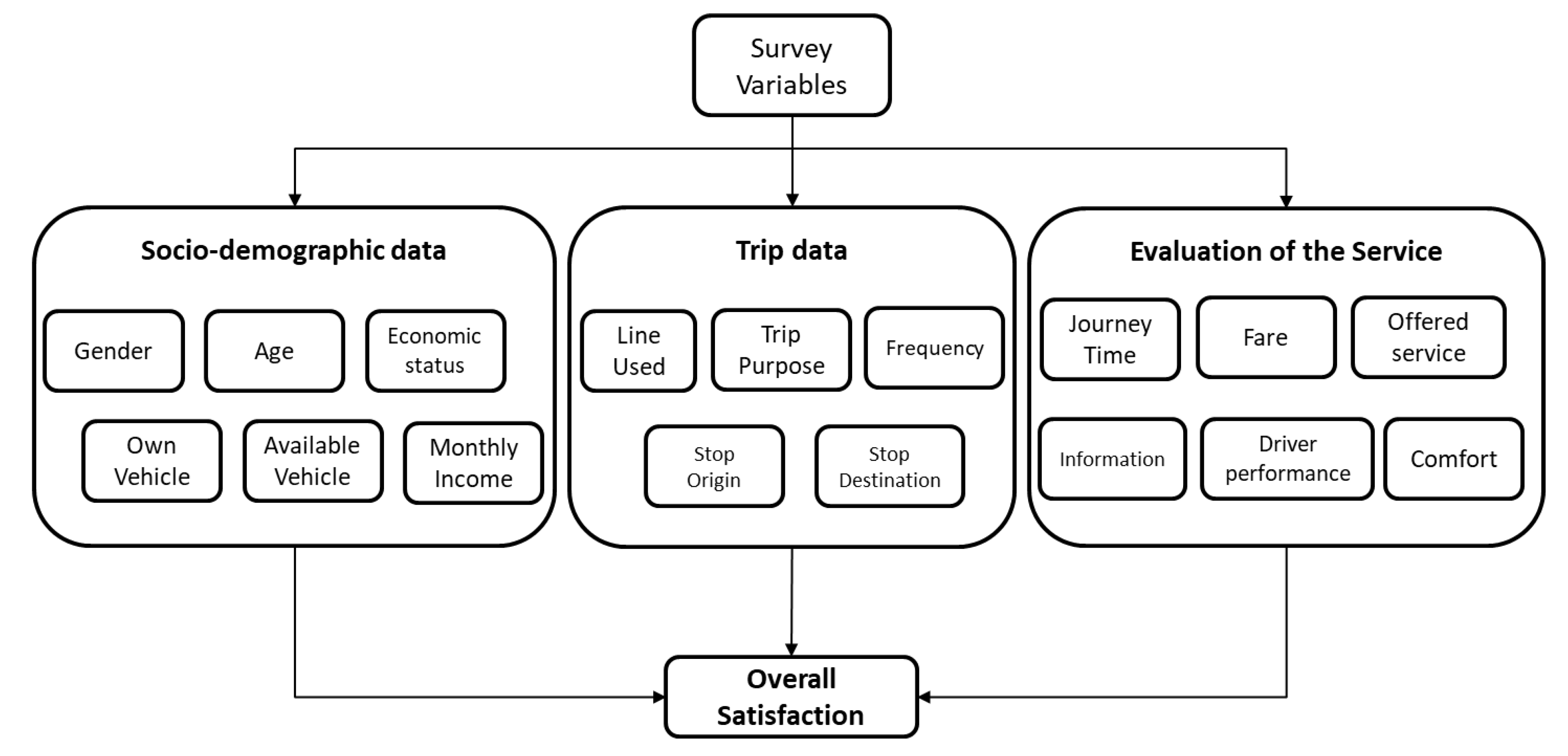
3.1. Perceived Quality (PQ) Survey

The PQ survey had three main goals: (1) to identify the socio-demographic characteristics of respondents, (2) to analyse trip characteristics and (3) to determine user-perceived quality and overall satisfaction with the public transport service. Accordingly, the questionnaire was split into three different sections (see also Figure 1 and

Table 1. Survey administered to public transport users.

Socio-Demographic Data		Trip Data
Gender	Female	Line Used		Line 1
Age	24 or younger			Line 2
	25 to 34 years old			Line 3
	35 to 44 years old			Line 13
	45 to 54 years old	End Trip Purpose		Home
	55 to 64 years old			Work
	65 or older			Study
Economic Status	Worker			Health
	Unemployed			Shopping
	Student			Leisure
	Retired			Other
Own Vehicle	Yes/No	Number of trips per week		<5
Available Vehicle	Yes/No			5–15
Monthly household income	≤900 €			15–30
	900–1500 €			>30
	1500–2500 €	Stop of Origin		Code
	>2500 €	Destination Stop		Code
	DK/NA *
Overall Satisfaction and perceived quality of service
Access time to the stop (AT)			Very Poor (0) Poor (1) Regular (2) Good (3) Very Good (4)
Waiting Time (WT)
Travel Time (TT)
Time from the stop to the destination (DT)
Ticket fare (PR)
Transfer easiness (TR)
Offered service (SE)
Reliability (punctuality) (SR)
Line Coverage (LC)
Information on stops (IS)
App Information (IM)
Web Information (IW)
On board Information (IB)
Occupancy level (OC)
Air conditioning/calefaction (CA)
Space for Persons with Reduced Mobility (RM)
Seats comfort (CM)
Cleanliness (CL)
Driving Style (DS)
Driver kindness (DK)
Use of Hybrid Technology (HY)
Quality of stops (ST)
Route map design (MD)
Noise (NO)
Overall satisfaction

* Don’t Know/No Answer.

). The first section was comprised of 6 questions regarding the socio-demographic backgrounds of the users. The second section contained questions regarding the usual trips performed by users and common aspects of the use of the public transport service. Finally, the third section involved users’ overall satisfaction with the service as well as their perceived quality concerning specific aspects, such as access time, travel time, fare, reliability and others. These responses were collected by using a five-point Likert scale: very poor (0), poor (1), regular (2), good (3) and very good (4).

The number of required respondents per bus line can be estimated as follows:

$$n\ge \frac{N\times z^2\times {\sigma }^2}{e^2(N-1)+z^2\times {\sigma }^2}$$

(1)

where, n is the minimum number of required responses per bus line, e is the maximum acceptable error, z is the desired level of confidence, N refers to the total number of travellers for the considered bus line and σ² is the variance in the population of the variable of interest.

3.2. Zoning

Once data are collected, the next step consists of delimiting homogenous zones or neighbourhoods and associating them with the answers obtained in the surveys.

This zoning of the study area was designed so that areas with homogenous socioeconomic, urban morphology and functional characteristics could be defined. The procedure involved firstly, the evaluation of the administrative divisions, i.e., district and census sections, which enables the evaluation of socioeconomic statistical data, such as population density, ageing or quality of life indexes. Later, these administrative boundaries were modified with attention paid to the analysis of urban patterns of development, including the geographical distribution of building typologies and their age, built-up density, green surface, free and leisure spaces, the existence and typology of facilities (schools, medical centres, etc.) and main land uses (residential, commercial, industrial or public services).

After that, the stops of origin of the surveyed users, and thus, their valuations, are related to the zonal division in order to study spatial disparities in user satisfaction.

3.3. The Ordered Probit Model

An ordered probit model is proposed to estimate users’ overall satisfaction, given that users’ perceptions have been measured by ordinal variables involving values between 0 and 4. The model’s formulation is as follows:

$$q_i^{*}={\mathsf{\beta }}^{\prime }{v}_i+{\epsilon }_i,i=1,\dots ,n,$$

(2)

where, i refers to each individual user, q_i* is the individual’s estimated utility, v_i is the vector of the independent or explanatory variables, β′ is the vector of parameters to be estimated and ε_i is the error, which is assumed to be normally distributed, with mean 0 and variance 1, when all individuals i are considered. The measurement of the continuous utility q_i* was discretely observed through the following censorship mechanism:

$$\begin{array}{l}{q}_i=0\mathrm{if}{\mu }_{-1}<q_i^{*}\le {\mu }_{0,}\hfill \\ q_i=1\mathrm{if}{\mu }_0<q_i^{*}\le {\mu }_{1,}\hfill \\ q_i=2\mathrm{if}{\mu }_1<q_i^{*}\le {\mu }_{2,}\hfill \\ q_i=\dots \hfill \\ q_i=J\mathrm{if}{\mu }_{J-1}<q_i^{*}\le {\mu }_{J.}\hfill \end{array}$$

(3)

where μ_j represents the threshold parameters to be estimated. This model has to be normalized in order to allow for the identifiability of the other parameters [44]. In the first place, to ensure positive probabilities, it is required that μ_j > μ_j−1. In the second place, given that utility is going to be measured in the real line, μ_j−1 = −∞ and μ_j = +∞. Thirdly, it is assumed that Var(ε_i|v_i) = 1, given that Var(ε_i) is unidentifiable. This normalization does not imply a loss of generality in the model, given that to scale μ_j and the parameter β, the same positive value preserves the results obtained. Finally, assuming that v_i contains a constant, then μ₀ = 0.

Taking into account these conditions, the probabilities of the model are given by the following expression:

$$Prob(q_i)=Prob\left({\mu }_{j-1}<q_i^{*}<{\mu }_j\right)=\Phi ({\mu }_j-{\mathsf{\beta }}^{\prime }{v}_i)-\Phi ({\mu }_{j-1}-{\mathsf{\beta }}^{\prime }{v}_i),j=0,1,\dots ,J$$

(4)

where Φ is the normal accumulated distribution, and β′ can be estimated by maximum likelihood, maximizing the following log-likelihood function:

$$\log L={\displaystyle \sum _i\ln (Prob(q_i))=}{\displaystyle \sum _i\ln (\Phi ({\mu }_j-{\mathsf{\beta }}^{\prime }{v}_i)-\Phi ({\mu }_{j-1}-{\mathsf{\beta }}^{\prime }{v}_i))}$$

(5)

The estimated β parameters allow obtaining the influence of the different variables on the satisfaction declared by the user. However, neither the sign nor the magnitude of the coefficients is directly informative of the partial effect of each independent variable in the dependent one. To calculate this effect, the specific partial effect of each variable must be estimated for each response level q_i.

4. Application of the Model to Santander

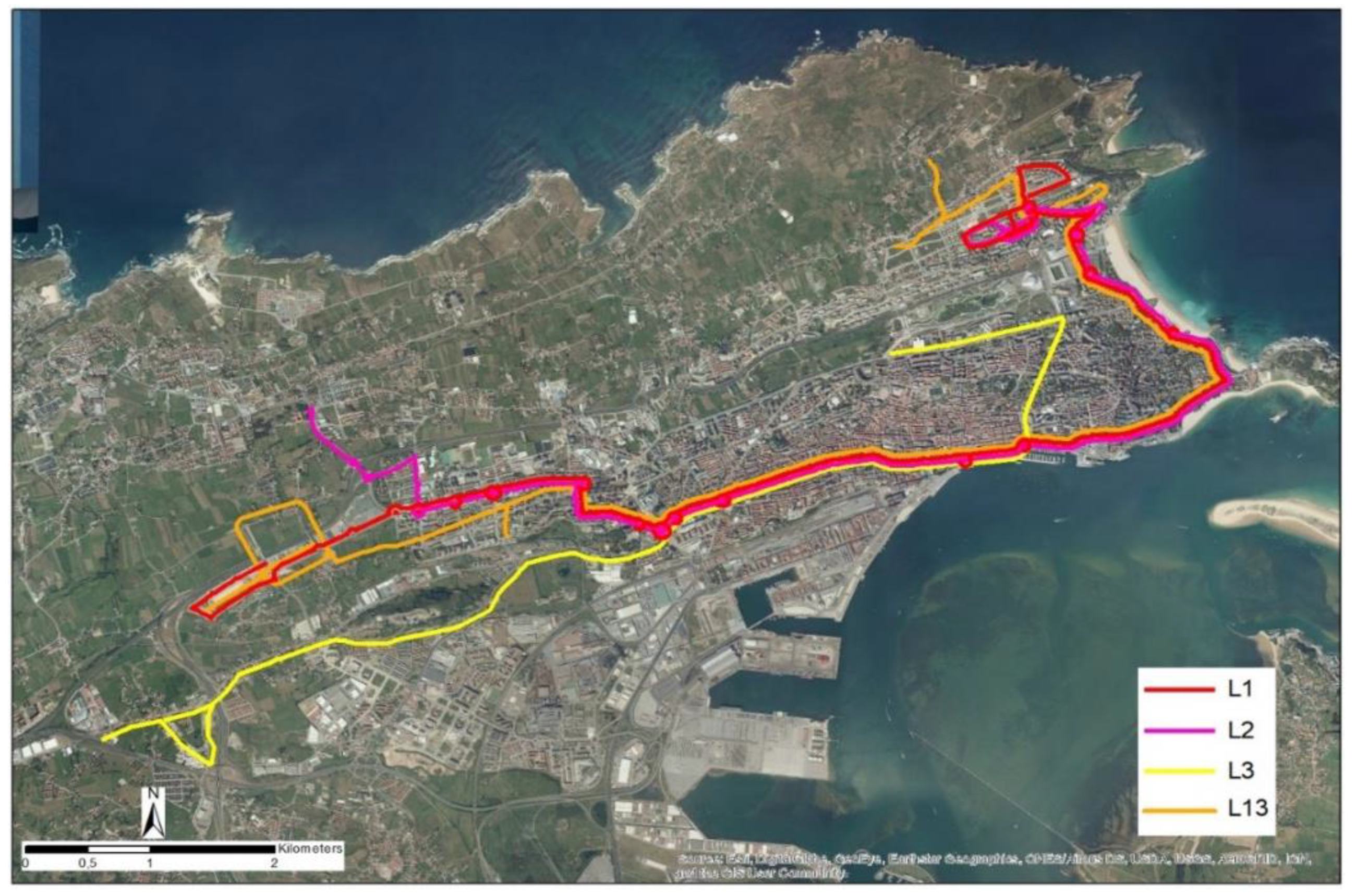
4.1. Case Study

The case study area for this investigation is the medium-sized city of Santander, the capital of the Cantabria region, situated in northern Spain. The Santander municipality has an expanse of around 35 km² and a population of 171,951 inhabitants as of 2017 [45]. Its urban public transport system consists of 20 bus lines, of which the four main ones: numbers 1, 2, 3 and 13, respectively (see Figure 2), connect the municipality from east to west, comprising 40% of the total users of this municipal service. These lines were selected since they have a quality certification (regulated by European Standard EN 13816) and data regarding users’ perception and satisfaction of the service was available for them.

4.2. Characterization of the Sample and Evaluation of Service Quality

The survey on users’ satisfaction with Santander’s transport system was conducted between 25 October and 23 November 2017. The questionnaire was administered to a total of 804 users, taking into account the minimum number of surveys estimated using (1), for a value of σ² of 0.4, an error level of 10% and a confidence level of 95% (

Table 2. Minimum number of required surveys and those eventually carried out.

Line	Minimum Surveys Required	Surveys Carried Out
1	150	217
2	149	226
3	146	193
13	144	168
Total	589	804

).

Sixty-seven percent of the individuals surveyed were women, a similar figure to that presented in previous studies, due to their higher use of public transport [46]. As for age range, younger users (under 24 years-old), were the largest stratum, while those over 65 were the ones who used public transport least. However, grouping the results into adult age ranges, 52% of users were between 25 and 64 (

Table 3. Summary of survey responses.

Socio-Demographic Data	Gender	Female	67%
	Age	24 or younger	25%
		25 to 34 years old	13%
		35 to 44 years old	16%
		45 to 54 years old	17%
		55 to 64 years old	16%
		65 or older	13%
	Work Status	Worker	51%
		Unemployed	85%
		Student	24%
		Retired	17%
	Own Vehicle	Yes	36%
	Available Vehicle	Yes	53%
	Monthly household income	≤900 €	7%
		900–1500 €	20%
		1500–2500 €	17%
		>2500 €	14%
		DK/NA *	42%
Trip Data	Line Used	Line 1	27%
		Line 2	28%
		Line 3	24%
		Line 13	21%
	End Trip Purpose	Home	29%
		Work	25%
		Study	12%
		Health	5%
		Shopping	7%
		Leisure	13%
		Other	9%
	Number of trips per week	<5	26%
		5–15	54%
		15–30	18%
		>30	2%
Overall Satisfaction and Perceived Quality of Service	Evaluation of the Service	Very Poor (0)	2%
		Poor (1)	5%
		Regular (2)	26%
		Good (3)	56%
		Very Good (4)	11%

* Don’t Know/No Answer.

). This percentage explains the values obtained for the question regarding work status, for which 51% of the respondents were active workers and 24% students. Considering the possession of a private vehicle, 36% of the respondents answered positively, while 53% indicated that they had a vehicle available, either as car drivers, companions or motorcycle users. Finally, considering the level of income, more than a third of the people surveyed belonged to a household with incomes between 900 and 2500 euros, although 42% of the users did not know or declined to answer this question.

Regarding trip type, more than 50% of the people surveyed used bus transport between five and 15 times per week, those making more than 30 trips per week being marginal. Of the total number of respondents, 72% were travelling to or from home. In addition, 29% of the trips had their origin at home, while 37% were for mandatory purposes (work and/or study).

Among the different attributes of evaluation of the perceived quality (

Table 4. Quality evaluation of different variables.

Name	Average Evaluation
Seats comfort (CM)	2.50
Reliability (SR)	2.31
Travel Time (TT)	2.30
Time from the stop to the destination (DT)	2.29
Space for Persons with Reduced Mobility (RM)	2.29
Access time to the stop (AT)	2.26
Information on stops (IS)	2.26
Driver kindness (DK)	2.22
Offered service (SE)	2.21
Route map design (MD)	2.18
Waiting Time (WT)	2.16
Cleanliness (CL)	2.16
Quality of stops (ST)	2.15
Line Coverage (LC)	2.14
Use of Hybrid Technology (HY)	2.13
Ticket fare (PR)	2.10
On board Information (IB)	2.07
Noise (NO)	2.06
Driving Style (DS)	2.05
Occupancy level (OC)	2.04
Transfer easiness (TR)	2.03
Air conditioning/calefaction (CA)	1.98
App Information (IM)	1.81
Web Information (IW)	1.70
Overall satisfaction	2.69

), the one with the highest average score was seat comfort (CM) with a rating of 2.5. On the opposite side was the information provided through the web (IW) or the mobile phone application (IM) that presented the lowest scores among users, with ratings between 1 (poor) and 2 (regular). The average overall satisfaction with the service was 2.7; that is, between regular and good.

4.3. Zoning and Differences in Overall Satisfaction by Area

The zoning of Santander resulted in the classification of 10 homogeneous areas (Figure 3). The first one, named 1—Centre, corresponds to the location of the first settlement of the city, mainly represented by traditional neighbourhoods showing some physical, social and economic deterioration. This zone also contains the expansion district of the 19th century, a high-class residential and shopping area. Thus, zone 1—Centre is the one with the highest density of housing and population and the highest concentration of services in the city. This area has its continuity towards the west, in the so-called zone 2—Centre entrance, a mainly residential area comprised by apartment blocks built between the 60 s and mid-70 s [47].

To the east, we find the area 3—Sardinero. Established as a leisure space since the 19th century [48], it is linked to touristic resources including urban beaches and green areas, and to the presence of detached dwellings arranged as a garden city which were traditionally meant as seasonal residences. This area, along with the residential zone 4—Valdenoja-Cueto, presents the highest welfare index [49], taking into account the state of the housing and environmental living conditions (natural light, environmental situation, security, etc.). Valdenoja, developed as of the mid-60s, and especially during the 80s, involved the expansion of the Sardinero area, incorporating and absorbing part of the traditional rural core of Cueto [47], through open block houses intended for medium–high income classes.

Area 5—Valdecilla-Cazoña—was also developed around the 1950s and the 70s. It is a residential area associated with the largest regional hospital. The building typology includes single-family homes in the so-called Garden City and open buildings for middle-class citizens that sought to get away from the high densities of the city centre and find sunnier homes in Cazoña [47].

Continuous to these developments, to the west, are two mixed areas which represent the expansion of the city. On the one hand, to the south, zone 6—Peñacastillo, comprised of a residential area located where the former village integrates with monofunctional land blocks of industrial and logistics areas linked to the N-611 Santander-Madrid road and new residential developments. This area presents the lowest wealth index in the city [49], due to housing and environmental problems, such as lack of natural light, noise, pollution and crime. On the other hand, is zone 7—El Alisal, where high-rise residential buildings coexist with commercial uses, large facilities, workshops and storage areas.

Farther north, Zone 8—Corbán exemplifies the recent expansion of the municipality towards the periphery. It is an area of traditional rural character in which urbanization based on single family or semi-detached houses developed mainly from 1991 and until the real estate crisis of 2008, configuring a low density, dispersed residential area, with few facilities.

Finally, we defined two activity areas, Zone 9—Castros, which corresponds to the main university campus of the region, and Zone 10—PCTCAN-Adarzo, which is the area of greatest economic activity. The latter area comprises the PCTCAN, a Scientific-Technological Park and a large commercial area. It is a sparsely populated area, where there are still many unbuilt plots and buildings associated to the rural settlement of Adarzo.

Once this delimitation into zones was concluded, the stops of origin of the surveyed users were related to each zone, and the average and standard deviation of satisfaction per zone was calculated (

Table 5. Average satisfaction with public transport lines per zone.

Zone	Average Satisfaction	Standard Deviation Satisfaction
1—Centre	2.73	0.75
2—Centre entrance	2.66	0.79
3—Sardinero	2.70	0.76
4—Valdenoja-Cueto	2.77	0.80
5—Valdecilla-Cazoña-Albericia	2.59	0.83
6—Peñacastillo	2.69	0.89
7-Alisal	2.70	0.74
8—Corbán	2.95	0.78
9—Castros	2.60	0.91
10—PCTCAN-Adarzo	2.48	0.88

). The satisfaction histogram was fairly similar among zones with a single modal value (evaluation—good). The spatial distribution of satisfaction shows how, although the average scores were in a range between 2.48 and 2.95, there was some spatial variability.

In order to visualize this spatial pattern, a service area was estimated for each stop using the pedestrian network, and specifying a walking time of 5 minutes and a walking speed of 3.6 km/h (Figure 4). The area with the worst-rating was 10—PCTCAN-Adarzo, while the one with the best valuations was the neighbouring 8—Corbán, to the northwest of the study area. This contrasting result can be related to both the diverse line coverage and characteristics of the service and the typology of the two neighbour zones; i.e. on the one hand, an economic area which attracts numerous workers and shoppers from all over the city and beyond, and on the other, a residential zone where rural settlements are combined with new residences that need access mainly to the city centre and only at certain departure and arrival times. The other areas, where user satisfaction was higher-than-the-average, were the very well connected 1—Centre and 4—Valdenoja-Cueto, a mainly residential zone.

Contrasting satisfaction with the service in neighbouring areas was also tested by the estimation of Moran’s I statistic, considering two, three and four nearest neighbours. In all cases, a negative value was obtained, clearly significant in the cases of two (−0.54) and three (−0.48) neighbours, suggesting a heterogeneous satisfaction among neighbouring areas. The reasons behind these discrepancies are investigated in detail next.

4.4. Results of the Ordered Probit Model

Once the results from the survey were discretized by zone, the next step of the methodology was the estimation of ordered probit models to check which spatial differences existed regarding customers’ preferences. The estimation of parameters was performed using maximum likelihood.

Table 6. Estimated parameters and t-tests (in brackets) of the ordered probit models.

Variable	Model 1	Model 2	Model 3	Model 4
Constant	−0.557 (−3.62)	−0.816 (−5.51)	−0.589 (−3.93)	−0.528 (−3.54)
Socio-demographic and trip data variables
Gender (Female)	−0.144 (−1.94)	−0.158 (−2.10)	−0.129 (−1.61)	−0.150 (1.72)
Income > 2500 €	0.352 (4.57)	0.370 (4.42)	0.342 (4.72)	0.358 (4.30)
Own Vehicle	−0.207 (−3.27)	−0.199 (−3.13)	−0.220 (−3.50)	−0.239 (3.90)
Available Vehicle	−0.339 (−2.50)	−0.330 (−2.38)	−0.350 (−2.41)	−0.335 (2.22)
Spatial variation socio-demographic and trip data variables
Income < 1500 € Z1	-	-	−0.147 (−2.65)	−0.330 (10.75)
Income < 1500 € Z4	-	-	−0.183 (−2.86)	−0.163 (4.43)
Income < 1500 € Z6	-	-	−0.532 (−9.53)	−0.676 (13.62)
Income < 1500 € Z7	-	-	0.219 (2.72)	-
Age > 65 years Z1	-	-	0.186 (3.96)	-
Age > 65 years Z2	-	-	−0.404 (−4.51)	−0.427 (−7.97)
Age > 65 years Z3	-	-	0.696 (8.90)	0.867 (21.53)
Age > 65 years Z5	-	-	0.190 (7.73)	0.257 (6.21)
Age > 65 years Z6	-	-	−0.513 (−7.99)	−0.647 (−10.58)
Age > 65 years Z7	-	-	−0.736 (−11.00)	−0.952 (−11.69)
Age > 65 years Z8	-	-	0.947 (7.82)	0.860 (14.04)
Age > 65 years Z9	-	-	−0.946 (−6.67)	-
Age > 65 years Z10	-	-	−0.694 (−6.65)	−0.705 (−8.40)
Trips ≥ 5 Z5	-	-	−0.276 (−5.97)	−0.121 (−1.68)
Trips ≥ 5 Z6	-	-	0.386 (6.10)	0.150 (3.33)
Zones
Z1	-	0.416 (22.46)	-	-
Z2	-	0.210 (12.41)	-	-
Z3	-	0.211 (12.19)	-	-
Z4	-	0.258 (8.55)	-	-
Z5	-	0.055 (1.74)	-	-
Z6		0.327 (11.13)
Z7	-	0.348 (10.32	-	-
Z8	-	0.512 (19.98)	-	-
Z9	-	0.169 (4.11)	-	-
Perceived quality of service
Access time to the stop (AT)	0.134 (4.99)	0.141 (5.06)	0.143 (4.80)	0.144 (4.98)
Travel Time (TT)	0.145 (4.87)	0.152 (5.00)	0.150 (5.82)	0.156 (5.56)
Transfer easiness (TR)	0.062 (2.50)	0.062 (2.48)	0.067 (2.87)	0.068 (3.12)
Offered service (SE)	0.109 (6.68)	0.111 (5.74)	0.109 (6.10)	-
Reliability (SR)	0.151 (3.90)	0.154 (3.91)	0.155 (3.97)	0.156 (4.02)
Line coverage (LC)	0.151 (4.38)	0.148 (4.11)	0.157 (4.74)	-
Information on stops (IS)	0.070 (5.97)	0.070 (5.90)	0.071 (6.14)	0.079 (7.06)
On board Information (IB)	0.101 (2.83)	0.099 (2.70)	0.110 (2.97)	0.110 (2.87)
Occupancy level (OC)	0.135 (9.07)	0.139 (8.10)	0.137 (8.02)	0.143 (7.41)
Space for Persons with Reduced Mobility (RM)	0.068 (2.50)	0.067 (2.53)	0.065 (2.49)	0.064 (2.54)
Driving Style (DS)	0.066 (2.76)	0.066 (2.55)	0.068 (2.95)	0.074 (3.34)
Use of Hybrid Technology (HY)	0.059 (2.05)	0.063 (2.04)	0.070 (2.25)	0.068 (2.08)
Noise (NO)	0.066 (2.86)	0.059 (2.14)	0.064 (2.49)	0.064 (2.20)
Quality of stops (ST)	0.053 (2.12)	0.060 (2.30)	0.050 (1.84)	0.059 (2.00)
Route map design (MD)	0.074 (3.53)	0.068 (2.97)	0.070 (3.18)	0.067 (2.62)
Spatial variation perceived quality of service
SE Z1	-	-	-	0.192 (6.94)
SE Z2	-	-	-	0.089 (3.78)
SE Z3	-	-	-	0.061 (2.85)
SE Z4	-	-	-	0.106 (4.25)
SE Z6	-	-	-	0.118 (4.97)
SE Z7	-	-	-	0.109 (3.92)
SE Z8	-	-	-	0.132 (4.16)
LC Z1	-	-	-	0.137 (6.45)
LC Z2	-	-	-	0.142 (5.08)
LC Z3	-	-	-	0.095 (3.40)
LC Z4	-	-	-	0.116 (4.47)
LC Z5	-	-	-	0.154 (7.39)
LC Z6	-	-	-	0.248 (10.55)
LC Z7	-	-	-	0.221 (8.26)
LC Z8	-	-	-	0.125 (5.89)
LC Z10	-	-	-	0.191 (4.48)
Threshold parameters
Mu (01)	0.704 (12.12)	0.715 (12.55)	0.716 (12.25)	0.725 (12.56)
Mu (02)	1.922 (37.89)	1.944 (38.30)	1.960 (40.09)	1.979 (39.06)
Mu (03)	3.851 (43.91)	3.891 (44.19)	3.933 (44.65)	3.971 (43.66)
Goodness of fit indicators
Log likelihood value	−820.03	−813.92	−806.16	−800.64
Restricted log likelihood	−917.28	−917.28	−917.28	−917.28
Chi squared	194.51	206.72	222.23	233.27
McFadden Pseudo R2	0.11	0.11	0.12	0.13
Likelihood Ratio Test versus basic model (p-value)	-	12 (0.21)	28 (0.02)	74 (0.00)
N	804	804	804	804

shows the estimated parameters along with their t-tests (in brackets). Models were all calculated using a robust covariance matrix, accounting for the likely correlations between observations within the same zone of origin.

All the available variables were first introduced within the models. In a second step, the parameters with low t-test values were interpreted as non-significant and removed from the model. The simplest model (Model 1) only considered explanatory variables related to the socio-demographic characteristics of the users, trip characteristics and perceptions on several attributes of the service (Table 6). Amongst the socio-demographic variables, owning or being able to use a private vehicle and being a female (two thirds of respondents), had a considerable negative influence on the overall satisfaction with the service, as in previous gender-related research [50]. Conversely, in those cases in which the user belonged to a high-income household (over 2500 €), there was a higher likelihood to declare a good level of satisfaction, in line with the results of the income model by Iseki and Smart [10] and in contrast with those obtained by Ji and Gao [30]. The other socio-demographic and trip variables, such as age, work status, line used and trip frequency were clearly not significant, and thus were removed from the utility function of the model.

Amongst the variables associated with perceived quality of the diverse attributes of the service, reliability (SR), line coverage (LC) and travel time (TT) had significant parameters and were the most relevant when accounting for overall satisfaction (Table 6). The three threshold parameters were clearly significant, and the goodness of fit of the model was 0.11, compared to the null model, according to McFadden’s pseudo R².

Model 2 was constructed by adding to Model 1, nine dummy variables referring to the locations of stops of origin according to the proposed zoning. Zone 10, PCTCAN-Adarzo, was chosen as the base level for dummy variables, since it was the zone with the lowest level of satisfaction. The parameters of the dummy variables were, therefore, positive in all cases. Higher parameters were obtained for Zone 1—Centre and Zone 8—Corbán, two areas with a high level of average satisfaction (Table 6). The remaining socio-demographic, trip and perceived quality variables obtained a similar magnitude and significance as those in Model 1 and reliability, travel time and coverage were also the variables with the highest relevance. The goodness of fit of Model 2 was somewhat superior to Model 1. Additionally, a likelihood ratio test (LR) was performed to check whether Model 2’s fitting was significantly better than that of Model 1, considering that nine additional variables were included. The value of the LR test was 12, rejecting the null hypothesis, at a confidence level of 95% according to the χ² distribution. Therefore, although dummy variables improved the goodness of fit of the model to the observed differences in users’ satisfaction in the various neighbourhoods, they did not provide a large explanatory component.

In Model 3, in addition to the socio-demographic and trip variables, their possible differential effect on space was included through their interaction with the dummy variables specified in Model 2. After testing different specifications, in order to select only significant interactions, it became apparent that people with incomes lower than 1500 €, older people (65 years old or older) and frequent users (five or more trips per week) showed differences in their satisfaction with the service according to the area of origin. Thus, lower income users from zones 1—Centre, 6—Peñacastillo and 4—Valdenoja-Cueto had a higher probability of being less satisfied with the service, ceteris paribus, and this was especially the case of users with their origin in zone 6 (Table 6), which is indeed the area with the lowest wealth index. In the case of people aged 65 or above, in zones 2—Centre entrance, 6—Peñacastillo, 7—Alisal, 9—Castros and 10—PCTCAN-Adarzo, their satisfaction was most likely lower than that of the other users. On the other hand, in zones 1—Centre, 3—Sardinero, 5—Valdecilla-Cazoña-Albericia and 8—Corbán, the probability that this type of user was more satisfied was higher. Finally, among people who used public transport more frequently, those located in zone 5-Valdecilla were more likely to be less satisfied with the service, while users from area 6—Peñacastillo were more likely to be pleased with it.

The consideration of this spatial variability in the satisfaction with the service of users with different socio-demographic characteristics and the use of public transport, allowed us to significantly improve the goodness of fit of the model. Thus, the LR test, performed with respect to Model 1, presented a value of 28 (clearly significant), at a confidence level of 95% according to the χ² distribution.

Finally, in Model 4, in addition to introducing the possible spatial variation of satisfaction according to socio-demographic and trip characteristics, the differential effects per zone were also considered when rating the importance of the different variables of the service. In two of the most relevant quality variables, offered service (SE) and line coverage (LC), a significant spatial variability was detected through its interaction with the zonal dummy variables (see the ‘Spatial variation in perceived quality of service’ section in Table 6). In the case of SE, its importance for overall satisfaction was especially high in zones 1—Centre and 8—Corbán. As for LC, it was more relevant for overall satisfaction in zones 6—Peñacastillo, 7—Alisal and 10—PCTCAN-Adarzo, the three of them are located in the western part of the city and involve economic areas, such as shopping centres and a research and technology centre. It is important to point out that in model 4, dummy variables for the lowest income people in zone 7—Alisal and for the elderly in zones 1—Centre and 9—Castros ceased to be significant. Therefore, the influence of having an income lower than 1500 € on overall satisfaction with the service was always negative in all areas where it was significant (zones 1, 4 and 6).

The goodness of fit of Model 4 was higher than that of the other models (log-likelihood: −800). However, the goodness of fit of this model cannot be compared with that of Model 1 through an LR test because Model 1 contains variables which were not present in Model 4 (SE and LC in Model 4 were considered different by area of origin instead of being included in their overall perceived quality). Even so, Model 4 was compared using an LR test with its restricted version without considering spatial variation in the socio-demographic and trip variables, or in the quality of service variables. In this case, the test presented a value of 74, clearly above the critical level, for a confidence level of 99% according to the χ² distribution.

In order to evaluate the relevance of the different variables analysed, their marginal effects on the probability of choosing between the different levels of overall satisfaction were calculated. For the highest level of satisfaction (very good—4), and considering the mean value of each variable (

Table 7. Estimated partial effects for the ordered probit model at the highest level of satisfaction (very good—4).

Variable	Model 1	Model 2	Model 3	Model 4
Socio-demographic variables and trip data variables
Gender (Female)	−0.022 (−2.04)	−0.023 (−2.17)	−0.018 (−1.66)	−0.021 (−1.61)
Income > 2500 €	0.061 (3.59)	0.063 (3.83)	0.056 (3.73)	0.058 (2.36)
Own Vehicle	−0.029 (−2.82)	−0.027 (−3.05)	−0.029 (−3.04)	−0.031 (−2.51)
Available Vehicle	−0.041 (−2.78)	−0.039 (−2.81)	−0.040 (−2.57)	−0.037 (−3.11)
Spatial variation socio-demographic and trip data variables
Income < 1500 € Z1	-	-	−0.018 (−2.48)	−0.036 (−1.88)
Income < 1500 € Z4	-	-	−0.022 (−2.66)	−0.020 (−0.77)
Income < 1500 € Z6	-	-	−0.050 (−6.21)	−0.056 (−4.50)
Income < 1500 € Z7	-	-	0.035 (2.54)	-
Age > 65 years Z1	-	-	0.029 (3.42)	-
Age > 65 years Z2	-	-	−0.042 (−4.22)	−0.042 (−1.81)
Age > 65 years Z3	-	-	0.149 (7.18)	0.199 (2.29)
Age > 65 years Z5	-	-	0.030 (6.97)	0.041 (0.62)
Age > 65 years Z6	-	-	-0.049 (−6.62)	−0.054 (−2.22)
Age > 65 years Z7	-	-	-0.059 (−8.03)	−0.063 (−4.77)
Age > 65 years Z8	-	-	0.231 (6.80)	0.198 (1.26)
Age > 65 years Z9	-	-	−0.065 (−6.61)	-
Age > 65 years Z10	-	-	−0.057 (−6.07)	−0.056 (−4.26)
Trips ≥ 5 Z5	-	-	−0.032 (−4.60)	−0.015 (−0.59)
Trips ≥ 5 Z6	-	-	0.068 (5.08)	0.022 (0.59)
Areas
Z1	-	0.071 (10.69)	-	-
Z2	-	0.033 (8.32)	-	-
Z3	-	0.033 (11.80)	-	-
Z4	-	0.042 (7.16)	-	-
Z5	-	0.008 (1.77)	-	-
Z6		0.056 (6.96)
Z7	-	0.061 (7.92)	-	-
Z8	-	0.099 (10.63)	-	-
Z9	-	0.027 (3.55)	-	-
Perceived quality of service
Access time to the stop (AT)	0.019 (6.20)	0.020 (4.99)	0.020 (5.73)	0.019 (4.18)
Travel Time (TT)	0.021 (4.16)	0.021 (4.44)	0.021 (5.19)	0.021 (4.26)
Transfer easiness (TR)	0.009 (2.76)	0.009 (2.65)	0.009 (3.23)	0.009 (2.09)
Offered service (SE)	0.016 (4.93)	0.016 (4.66)	0.015 (4.81)	-
Reliability (SR)	0.022 (3.08)	0.022 (3.16)	0.021 (3.18)	0.021 (4.24)
Line coverage (LC)	0.022 (4.47)	0.021 (3.82)	0.022 (5.01)	-
Information on stops (IS)	0.010 (6.81)	0.010 (5.89)	0.010 (6.44)	0.011 (2.29)
On board Information (IB)	0.015 (2.86)	0.014 (2.72)	0.015 (2.87)	0.015 (3.05)
Occupancy level (OC)	0.020 (5.35)	0.020 (6.45)	0.019 (5.12)	0.019 (3.70)
Space for Persons with Reduced Mobility (RM)	0.010 (2.22)	0.010 (2.45)	0.009 (2.22)	0.009 (1.92)
Driving Style (DS)	0.010 (2.40)	0.009 (2.33)	0.009 (2.53)	0.010 (2.17)
Use of Hybrid Technology (HY)	0.008 (2.00)	0.009 (2.01)	0.010 (2.22)	0.009 (2.19)
Noise (NO)	0.009 (2.87)	0.008 (2.20)	0.009 (2.56)	0.009 (1.71)
Quality of stops (ST)	0.008 (2.16)	0.008 (2.48)	0.007 (1.92)	0.008 (1.77)
Route map design (MD)	0.011 (3.26)	0.010 (2.84)	0.010 (2.90)	0.009 (1.86)
Spatial variation perceived quality of service
SE Z1	-	-	-	0.026 (2.96)
SE Z2	-	-	-	0.012 (1.03)
SE Z3	-	-	-	0.008 (0.82)
SE Z4	-	-	-	0.014 (1.40)
SE Z6	-	-	-	0.016 (1.14)
SE Z7	-	-	-	0.015 (1.11)
SE Z8	-	-	-	0.018 (1.08)
LC Z1	-	-	-	0.019 (2.16)
LC Z2	-	-	-	0.019 (2.25)
LC Z3	-	-	-	0.013 (1.26)
LC Z4	-	-	-	0.016 (1.59)
LC Z5	-	-	-	0.021 (1.92)
LC Z6	-	-	-	0.034 (2.37)
LC Z7	-	-	-	0.030 (1.61)
LC Z8	-	-	-	0.017 (1.08)
LC Z10	-	-	-	0.026 (2.46)

), the attributes of perceived quality reliability (SR), travel time (TT) and line coverage (LC) presented higher marginal effects on the probability of attaining the highest level of satisfaction. The effect of incomes higher than 2500 € (0.061) was also important, and it is notable that no variable had a marginal effect greater than 0.1. The attributes with a lower marginal effect were those corresponding to perceived quality, such as transfer easiness (TR), the presence of hybrid technology (HY) and stop quality (ST).

The marginal effects estimated in Model 2 were very similar to those calculated in Model 1, although in this case, users from zones 1—Centre, 7—Alisal and 8—Corbán, were more likely to be very satisfied with public transport (Table 7). This greater satisfaction was especially notable in the case of zone 8, whose parameter had an effect on the probability of being very satisfied close to 0.1.

In Model 3, the spatial variability in the socio-demographic and trip variables showed how individuals with the lowest incomes in zones 4—Valdenoja-Cueto and 6—Peñacastillo presented a negative marginal effect on the probability of having a high satisfaction (Table 7). On the contrary, the older users in the 3—Sardinero and 8—Corbán areas had a high positive marginal effect on probability, as a consequence of their high satisfaction with the service. This finding is in line with the results of Mouwen [51], in which users over 65 showed a higher overall satisfaction with public transport. The users with the highest frequency of bus use in zone 6 also had a high marginal effect (0.068) on the probability of being very satisfied with the service.

In Model 4, the spatial variation in the perceived quality of the service showed important differences in the marginal effects of different zones, and therefore, in the importance given to this variable. Thus, the marginal effects in zone 1—Centre for the offered service (SE) and in zone 6—Peñacastillo for LC were highest, while those in zone 3—Sardinero, both for SE and LC, were lowest (Table 7).

The information provided by Models 3 and 4 regarding service quality, can be synthesized graphically following the quadrant analysis method proposed by Foote and Stuart [52] and Rojo et al. [46]. In Figure 5, the relevance of the different variables is represented in the x-axis according to the estimation of the marginal effect of Models 3 (in red) and 4 (in blue) for the highest level of satisfaction, while the average evaluation given by the users in the survey is represented on the y-axis. The average of both variables allows gathering them into four groups or quadrants.

-

Quadrant 1: variables which must be improved with the highest priority given that they present a higher relevance and lower valuation than the average.

-

Quadrant 2: variables that have a relevance and quality perception above the average, so it is convenient to keep them in that quadrant, (i.e., quality level).

-

Quadrant 3: variables with relevance and average valuations lower than the average. Therefore, they are characteristics of the service that can be improved, although with a lower priority than those present in zone 1.

-

Quadrant 4: variables with a relevance below the average and a higher than average valuation. Therefore, they are characteristics of the transport system with the lowest priority of action.

The quadrant analysis carried out presents the novelty, compared to previous studies, of allowing one to detect not only characteristics of the service that should be improved but also those spatial areas were action should be a priority. In this way, in Model 3, the variable LC (line coverage) presents a high priority, while SE (offered service) has one of the lowest priorities. However, Model 4 has distinguished the evaluation and relevance of the LC and SE variables by area, so it is possible to determine that the highest priorities for action on the coverage of the lines correspond to the zones 6—Peñacastillo and 10—PCTCAN-Adarzo, located in the western part of the study area. The coverage of lines in zone 7—Alisal, also located in the western area of the city, although with a slightly higher rating than the average, could also benefit from improvement. On the other hand, the improvement of SE, although not a priority in most areas, was rated well below the average in zone 2—Centre entrance, and especially in zone 1—Centre, and thus calls for action in these areas. A similar conclusion regarding the increase in efforts to improve services in central areas of the city, where satisfaction was lower than in peripheral ones, was reached by Ji and Gao [30].

4.5. Model Fitting According to Differences in Satisfaction per Zone

In order to verify the ability of the four estimated models to reproduce zonal differences in satisfaction with the service, their mean squared and absolute errors with respect to the answers given by the users were calculated.

Table 8. Goodness of fit of the estimated models to average satisfaction by zone.

Zone	Overall Satisfaction	Model 1	Model 2	Model 3	Model 4
1	2.73	2.83	2.89	2.83	2.90
2	2.66	2.84	2.81	2.84	2.85
3	2.70	2.91	2.91	2.93	2.90
4	2.77	2.96	2.96	2.92	2.91
5	2.59	2.88	2.80	2.85	2.79
6	2.69	2.85	2.90	2.88	2.87
7	2.70	2.89	2.92	2.89	2.89
8	2.95	2.95	2.98	3.00	3.00
9	2.60	2.89	2.80	2.86	2.69
10	2.48	2.84	2.74	2.81	2.77
Variance	0.015	0.002	0.006	0.003	0.008
Mean Squared Error	-	0.047	0.037	0.043	0.033
Mean Absolute Error	-	0.196	0.183	0.192	0.169

shows how Model 4 presents the lowest squared mean and absolute error of the four estimated models; that is, it is the one that best reproduces the average overall satisfaction of the users in the different zones. The basic model, without considering any type of spatial variability, presented a very low zonal variance in satisfaction with the service, clearly lower than that calculated from the data. This indicates that this model fails to capture spatial differences in satisfaction of the users. On the other hand, the models specified with dummy variables managed to capture the spatial variability of satisfaction better, Model 4 having a higher variance, closer to that calculated from the data.

5. Conclusions

Little attention has been given to the spatial variations in user satisfaction regarding public transport services. Although recent literature has confirmed that levels of satisfaction and their determining factors differ between regions [7], cities [53,54] or geographical areas, depending on their size and diverse attributes, the study of this diversity within cities, has hardly been addressed (with exceptions such as Ji and Gao [30]).

The present work studied which factors explain the spatial differences in overall satisfaction with public transport services in an urban area. To do so, data obtained from a perceived quality survey carried out in Santander were related to a neighbourhood zoning of the study area based on socio-demographic and urban quality aspects, by the estimation of ordered probit models. The models obtained have taken into account the existence of spatial divergences when estimating the influence of both the socio-demographic and trip variables of the users and each user’s individual perception of the importance of each variable in overall satisfaction.

In general, data showed that women and people owning or with access to a private vehicle are more likely to be less satisfied with the service. In contrast, wealthier people are more likely to show a high satisfaction with the public transport system. However, results also allowed us to confirm that there were significant differences in overall satisfaction between the delimitated neighbourhoods and that some socio-demographic and trip variables were only relevant for certain areas.

The use of dummy variables to capture spatial differences in perceived satisfaction allowed us to improve the goodness of fit of the models in both the overall evaluation and the valuations considering the different neighbourhoods. The interaction between dummy variables representing different zoning delimitations with socio-demographic, trip and perceived quality of service variables also enabled to identify factors explaining the variability in satisfaction levels. In this way, people with lower incomes, showed a lower likelihood of being satisfied with the service, in some specific areas, while in contrast, elderly people (over 65) were more likely to be satisfied in two specific neighbourhoods. This methodology also allowed us to detect that the significance given to certain variables is different in regard to the type of neighbourhood. This was the case for offered service (SE), which was especially relevant and poorly evaluated by users from the central urban area, while for users from western peripheral neighbourhoods, it was the line coverage (LC) that was poorly rated. These results indicate that users coming from peripheries, especially those with a high economic activity, want a service that grants them access to more destinations, mainly due to the fact that the current system favours the periphery-centre connection excessively, while users from the city-centre, who are, in general, well connected with all neighbourhoods, valued most, a higher frequency of services.

The modelling performed considering differences in satisfaction between different neighbourhoods, according both to the different types of users and to variations in the relevance given to the various attributes of the service, turned out to be a useful approach to identify those places where improving transport systems is more critical. Therefore, it is advisory to take into account the existence of spatial disparities when estimating users’ overall satisfaction, in order to identify neighbourhoods with differing perceptions with respect to the city’s average satisfaction with the system. Detecting unsatisfied neighbourhoods could help to take notice of deficiencies on certain perceived aspects of the service that, if corrected, could improve user satisfaction, and consequently, increase the demand of public transport. Since the use of public transport systems is seen as a key component of sustainable cities, understanding spatial differences in satisfaction will help planners and decision-makers to prioritise their investments and adapt their policies to specifically disadvantaged users and urban areas, thus achieving a more equitable, efficient and less polluting mobility.

References

1. Tao, S.; Corcoran, J.; Mateo-Babiano, I.; Rohde, D. Exploring Bus Rapid Transit passenger travel behaviour using big data. Appl. Geogr. 2014, 53, 90–104. [Google Scholar] [CrossRef]
2. Holmgren, J. Meta-analysis of public transport demand. Transp. Res. Part A Policy Pract. 2007, 41, 1021–1035. [Google Scholar] [CrossRef] [Green Version]
3. Redman, L.; Friman, M.; Gärling, T.; Hartig, T. Quality attributes of public transport that attract car users: A research review. Transp. Policy 2013, 25, 119–127. [Google Scholar] [CrossRef]
4. Buehler, R.; Pucher, J. Demand for public transport in Germany and the USA: An analysis of rider characteristics. Transp. Rev. 2012, 32, 541–567. [Google Scholar] [CrossRef]
5. Marcucci, E.; Gatta, V. Quality and public transport service contracts. Eur. Transp. 2007, 36, 92–106. [Google Scholar]
6. Chowdhury, S.; Hadas, Y.; Gonzalez, V.A.; Schot, B. Public transport users’ and policy makers’ perceptions of integrated public transport systems. Transp. Policy 2018, 61, 75–83. [Google Scholar] [CrossRef]
7. Abenoza, R.F.; Cats, O.; Susilo, Y.O. Travel satisfaction with public transport: Determinants, user classes, regional disparities and their evolution. Transp. Res. Part A Policy Pract. 2017, 95, 64–84. [Google Scholar] [CrossRef] [Green Version]
8. Dell’olio, L.; Ibeas, A.; Cecín, P. Modelling user perception of bus transit quality. Transp. Policy 2010, 17, 388–398. [Google Scholar] [CrossRef]
9. De Oña, J.; de Oña, R.; Calvo, F.J. A classification tree approach to identify key factors of transit service quality. Expert Syst. Appl. 2012, 39, 11164–11171. [Google Scholar] [CrossRef]
10. Iseki, H.; Smart, M. How do people perceive service attributes at transit facilities? Examination of perceptions of transit service by transit user demographics and trip characteristics. Transp. Res. Record 2012, 2274, 164–174. [Google Scholar] [CrossRef]
11. Morton, C.; Caulfield, B.; Anable, J. Customer perceptions of quality of service in public transport: Evidence for bus transit in Scotland. Case Stud. Transp. Policy 2016, 4, 199–207. [Google Scholar] [CrossRef]
12. Dell’olio, L.; Ibeas, A.; de Oña, J.; de Oña, R. Public Transportation Quality of Service: Factors, Models, and Applications; Elsevier: Cambridge, MA, USA, 2017; p. 242. [Google Scholar]
13. Parasuraman, A.; Zeithaml, V.A.; Berry, L.L. Servqual: A multiple-item scale for measuring consumer perc. J. Retail. 1988, 64, 12. [Google Scholar]
14. Grönroos, C. A service quality model and its marketing implications. Eur. J. Mark. 1984, 18, 36–44. [Google Scholar] [CrossRef]
15. Tyrinopoulos, Y.; Aifadopoulou, G. A complete methodology for the quality control of passenger services in the public transport business. Eur. Transp. 2008, 38, 1–16. [Google Scholar]
16. De Oña, J.; de Oña, R.; Diez-Mesa, F.; Eboli, L.; Mazzulla, G. A composite index for evaluating transit service quality across different user profiles. J. Public Transp. 2016, 19, 128–153. [Google Scholar] [CrossRef]
17. Filipović, S.; Tica, S.; Živanović, P.; Milovanović, B. Comparative analysis of the basic features of the expected and perceived quality of mass passenger public transport service in Belgrade. Transport 2009, 24, 265–273. [Google Scholar] [CrossRef]
18. Lai, W.-T.; Chen, C.-F. Behavioral intentions of public transit passengers—The roles of service quality, perceived value, satisfaction and involvement. Transp. Policy 2011, 18, 318–325. [Google Scholar] [CrossRef]
19. Tyrinopoulos, Y.; Antoniou, C. Public transit user satisfaction: Variability and policy implications. Transp. Policy 2008, 15, 260–272. [Google Scholar] [CrossRef]
20. Jomnonkwao, S.; Ratanavaraha, V. Measurement modelling of the perceived service quality of a sightseeing bus service: An application of hierarchical confirmatory factor analysis. Transp. Policy 2016, 45, 240–252. [Google Scholar] [CrossRef]
21. Rojo, M.; dell’Olio, L.; Gonzalo-Orden, H.; Ibeas, Á. Interurban bus service quality from the users’ viewpoint. Transp. Plan. Technol. 2013, 36, 599–616. [Google Scholar] [CrossRef]
22. Vetrivel Sezhian, M.; Muralidharan, C.; Nambirajan, T.; Deshmukh, S. Attribute-based perceptual mapping using discriminant analysis in a public sector passenger bus transport company: A case study. J. Adv. Transp. 2014, 48, 32–47. [Google Scholar] [CrossRef]
23. Conies, E.; Novales, M.; Orro, A.; Anta, J. Buses with High Level of Service in Nantes, France: Characteristics and Results of the BusWay Compared with Light Rail Transit. Transp. Res. Rec. 2014, 2418, 66–73. [Google Scholar] [CrossRef]
24. Chung, Y.-S.; Wong, J.-T. Developing effective professional bus driver health programs: An investigation of self-rated health. Accid. Anal. Prev. 2011, 43, 2093–2103. [Google Scholar] [CrossRef]
25. Ratanavaraha, V.; Jomnonkwao, S. Model of users’ expectations of drivers of sightseeing buses: Confirmatory factor analysis. Transp. Policy 2014, 36, 253–262. [Google Scholar] [CrossRef]
26. Del Castillo, J.; Benitez, F.G. A methodology for modeling and identifying users satisfaction issues in public transport systems based on users surveys. Procedia Soc. Behav. Sci. 2012, 54, 1104–1114. [Google Scholar] [CrossRef]
27. Sañudo, R.; Echaniz, E.; Alonso, B.; Cordera, R. Addressing the Importance of Service Attributes in Railways. Sustainability 2019, 11, 3411. [Google Scholar] [CrossRef]
28. Guirao, B.; García-Pastor, A.; López-Lambas, M.E. The importance of service quality attributes in public transportation: Narrowing the gap between scientific research and practitioners’ needs. Transp. Policy 2016, 49, 68–77. [Google Scholar] [CrossRef]
29. Dell’olio, L.; Ibeas, A.; Cecin, P. The quality of service desired by public transport users. Transp. Policy 2011, 18, 217–227. [Google Scholar] [CrossRef]
30. Ji, J.; Gao, X. Analysis of people’s satisfaction with public transportation in Beijing. Habitat Int. 2010, 34, 464–470. [Google Scholar] [CrossRef]
31. Kuo, C.W.; Tang, M.L. Relationships among service quality, corporate image, customer satisfaction, and behavioral intention for the elderly in high speed rail services. J. Adv. Transp. 2013, 47, 512–525. [Google Scholar] [CrossRef]
32. De Oña, J.; de Oña, R.; Eboli, L.; Mazzulla, G. Perceived service quality in bus transit service: A structural equation approach. Transp. Policy 2013, 29, 219–226. [Google Scholar] [CrossRef]
33. Bordagaray, M.; dell’Olio, L.; Ibeas, A.; Cecín, P. Modelling user perception of bus transit quality considering user and service heterogeneity. Transp. A Transp. Sci. 2014, 10, 705–721. [Google Scholar] [CrossRef]
34. Kim, Y.K.; Lee, H.R. Customer satisfaction using low cost carriers. Tour. Manag. 2011, 32, 235–243. [Google Scholar] [CrossRef]
35. Eboli, L.; Mazzulla, G. Service quality attributes affecting customer satisfaction for bus transit. J. Public Transp. 2007, 10, 21–34. [Google Scholar] [CrossRef]
36. De Oña, J.; de Oña, R. Quality of service in public transport based on customer satisfaction surveys: A review and assessment of methodological approaches. Transp. Sci. 2014, 49, 605–622. [Google Scholar] [CrossRef]
37. Allen, J.; Eboli, L.; Forciniti, C.; Mazzulla, G.; Ortúzar, J.D.D. The role of critical incidents and involvement in transit satisfaction and loyalty. Transp. Policy 2019, 75, 57–69. [Google Scholar] [CrossRef]
38. Paquette, J.; Bellavance, F.; Cordeau, J.-F.; Laporte, G. Measuring quality of service in dial-a-ride operations: The case of a Canadian city. Transportation 2012, 39, 539–564. [Google Scholar] [CrossRef]
39. Yaya, L.H.P.; Fortià, M.F.; Canals, C.S.; Marimon, F. Service quality assessment of public transport and the implication role of demographic characteristics. Public Transp. 2015, 7, 409–428. [Google Scholar] [CrossRef]
40. Hensher, D.A. The relationship between bus contract costs, user perceived service quality and performance assessment. Int. J. Sustain. Transp. 2014, 8, 5–27. [Google Scholar] [CrossRef]
41. Verbich, D.; El-Geneidy, A. The pursuit of satisfaction: Variation in satisfaction with bus transit service among riders with encumbrances and riders with disabilities using a large-scale survey from London, UK. Transp. Policy 2016, 47, 64–71. [Google Scholar] [CrossRef]
42. Cardamone, A.S.; Eboli, L.; Forciniti, C.; Mazzulla, G. Willingness to use mobile application for smartphone for improving road safety. Int. J. Inj. Control Saf. Promot. 2016, 23, 155–169. [Google Scholar] [CrossRef] [PubMed]
43. Stephen Cardamone, A.; Eboli, L.; Forciniti, C.; Mazzulla, G. How usual behaviour can affect perceived drivers’ psychological state while driving. Transport 2017, 32, 13–22. [Google Scholar] [CrossRef]
44. Greene, W.H.; Hensher, D.A. Modeling Ordered Choices: A Primer; Cambridge University Press: Cambridge, UK, 2010. [Google Scholar]
45. ICANE. Padrón Municipal de Habitantes; Instituto Cántabro de Estadística (ICANE): Santander, Spain, 2018. [Google Scholar]
46. Rojo, M.; Gonzalo-Orden, H.; Dell’Olio, L.; Ibeas, A. Modelling gender perception of quality in interurban bus services. Proc. Inst. Civ. Eng. Transp. 2011, 164, 43–53. [Google Scholar] [CrossRef]
47. Medina, A. Promoción Inmobiliaria y Crecimiento Espacial: Santander 1955–1974; Universidad de Cantabria: Santander, Spain, 2004. [Google Scholar]
48. Pozueta, J. El Proceso de Urbanización Turística. La Producción Del Sardinero. Ph.D. Thesis, Universidad de Cantabria, Santander, Spain, 1980. [Google Scholar]
49. Inguanzo, A.; Barreda, M.R.; Cordera, R.; Canales, C.; Reques, P. Las desigualdades socio-espaciales en la ciudad de Santander en relación a la población, bienestar y dotación de equipamientos sociales. In Despoblación, Envejecimiento y Territorio: Un Análisis sobre la Población Española; López, L., Abellán, A., Godenau, D., Eds.; Servicio de Publicaciones: León, Spain, 2009; pp. 719–730. (In Spanish) [Google Scholar]
50. Beirão, G.; Cabral, J.S. Market segmentation analysis using attitudes toward transportation: Exploring the differences between men and women. Transp. Res. Rec. 2008, 2067, 56–64. [Google Scholar] [CrossRef]
51. Mouwen, A. Drivers of customer satisfaction with public transport services. Transp. Res. Part A Policy Pract. 2015, 78, 1–20. [Google Scholar] [CrossRef]
52. Foote, P.; Stuart, D. Customer satisfaction contrasts: Express versus local bus service in Chicago’s North Corridor. Transp. Res. Rec. 1998, 1618, 143–152. [Google Scholar] [CrossRef]
53. Diana, M. Measuring the satisfaction of multimodal travelers for local transit services in different urban contexts. Transp. Res. Part A Policy Pract. 2012, 46, 1–11. [Google Scholar] [CrossRef] [Green Version]
54. Friman, M.; Fellesson, M. Service supply and customer satisfaction in public transportation: The quality paradox. J. Public Transp. 2009, 12, 57–69. [Google Scholar] [CrossRef]
Figure 1. Types of variables considered.
Sustainability 11 05829 g001
Figure 2. Bus lines studied.
Sustainability 11 05829 g002
Figure 3. Population density, zones and bus stops in the Santander area. Source: Population Census, 2011.
Sustainability 11 05829 g003
Figure 4. Average satisfaction per zone.
Sustainability 11 05829 g004
Figure 5. Relevance–valuation relationship for quality service variables in Models 3 (red) and 4 (blue).
Sustainability 11 05829 g005