Abstract
Cap-and-trade regulation is an effective mechanism to control carbon emissions. The optimization problem for a two-stage supply chain consisting of a manufacturer and a retailer under cap-and-trade regulation was investigated in this paper. Consumers’ low-carbon awareness level was considered in the decision models. Optimal decision policies, corresponding emissions, and profits were calculated for decentralized and centralized decision-making modes. Under a decentralized mode, the two-stage supply-chain optimization problem was formulated as a Stackelberg game model, where the manufacturer and retailer were the leader and follower, respectively. The manufacturer decides the emission-reduction levels per product unit and the retailer decides the retail price per unit product. The optimal decisions are derived using the reverse-solution method. By contrast, the two-stage supply-chain optimization problem under a decentralized mode was formulated as a single-level optimization model. The nonlinear model is handled by KKT optimality conditions. The influence of the regulation parameters (caps and carbon prices) and consumers’ low-carbon awareness on the optimal decision policies, the corresponding emissions, and profits is discussed in detail. A comparison between the two modes implies that the decentralized mode is dominated by the centralized mode in terms of profit and emissions. In order to provoke the decision makers under decentralized modes to make the decisions under the decentralized mode, a profit-sharing contract was designed. This study shows that higher consumer low-carbon awareness and carbon prices can improve the manufacturer-decision flexibility when there exists a profit-sharing contract. Finally, numerical experiments confirmed the analytical results.
1. Introduction
Increasing carbon emissions (emissions from greenhouse gases) have become a global issue due to their serious consequences. According to the report of Intergovernmental Panel on Climate Change (IPCC), industrial carbon dioxide emissions in 2050 must be 75% to 90% lower than those in 2010 to achieve the goal of controlling the rise of temperature within C. To achieve the C temperature control target, global climate action urgently needs to be accelerated. Faced with this grim situation, governments have to formulate various regulations to control emissions. Among these regulations, the cap-and-trade mechanism driven by market power is regarded as the most widely used policy tool [1,2,3]. The European Union Emissions Trading System (EU ETS) was launched in 2005 and it is the first international system for trading greenhouse-gas-emission allowances. Moreover, China established a national carbon-trading market for power-generation companies at the end of 2017. The cap-and-trade mechanism, which was put forward by the Kyoto Protocol [4], integrates regulatory and market power. This mechanism makes full use of market power to price carbon-emission permits so that superemission firms pay a price, while less-emission firms are profitable, and then guides low-carbon technological progress and investment in low-carbon projects, ultimately achieving low-carbon economic transformation.
As important sources of carbon emissions, firms must act in response to government emission regulations; otherwise, they are severely punished. Firms can achieve emission reduction in two aspects, technology upgrades and operation optimization. On the aspect of technology, firms can use more energy-efficient equipment and facilities, cleaner energy, and more environmentally friendly raw materials. Firms can also dispose of carbon emissions by postprocessing, such as Carbon Capture and Sequestration (CSS) technologies [5]. By March 2012, the Global CCS Institute had identified 75 large-scale integrated projects globally (http://www.ccsassociation.org/why-ccs/industry-experience/). All these emission-reduction technologies need extra investment. Apart from the aspect of technology, it is possible for firms to reduce emissions through individually optimizing operations [6]. For example, a logistics firm can change its carbon emissions by adjusting transport routes, the location of distribution centers, and delivering frequency. It should be noted that the effect of self-interested emission-reduction action of a firm is limited since a firm is part of a supply chain. The actions of members in a supply chain, individually reducing emissions without coordination with other members, are unlikely to achieve the target of minimizing the emissions of the entire supply chain. Taking a cold chain as an example, a retailer requires rapid delivering to address the growing expectations of consumers. In order to satisfy retailer requirements, a supplier has to build more cold-storage facilities and more vehicles with refrigeration systems, leading to more carbon emissions. Therefore, coordination among members in a supply chain should not be ignored. Within a supply chain, the self-interested behavior of decision makers can be bridged to some extent by contracts [7].
Faced with climate change caused by increasing carbon emissions, not only governments and firms but also ordinary consumers are changing their perceptions. Their environmental awareness is growing and they are increasingly inclined toward environmentally friendly products, which means that they are willing to pay more for these products in contrast with ordinary products. Toyota reported that its hybrid cars contribute to carbon dioxide reduction and are priced more than 1.5 times the price of their gasoline-powered counterparts [8]. Consumers are willing to pay higher prices for environmentally friendly products because they believe that their actions can benefit them, e.g., by promoting a healthy environment. In this study, environmental awareness is expressed as low-carbon awareness. To obtain premiums from consumer low-carbon awareness, carbon-labeling projects have been or are being developed in many countries. For example, Carbon Trust, a UK company, launched the first batch of carbon-labeling projects in 2007, including potato chips and shampoos. China has also formulated the General Rules for the Evaluation of Carbon Labels for Electrical and Electronic Products in China. Liu et al. [9] used literature review to discuss the evolution of the carbon-labeling concept, and different measurement methodologies and standards for carbon labels.
From this background, the decision makers in supply chains must take emission regulations and consumers’ low-carbon awareness into account. This study establishes two-stage supply-chain optimization models involving cap-and-trade regulation and consumers’ low-carbon awareness. Specifically, the following issues are investigated: (1) What are the optimal decisions for decision maker(s) under different modes? (2) How are optimal decisions, profits, and emissions influenced by regulation parameters and low-carbon awareness level? (3) How are decisions transferred from decentralized to centralized mode?
In this study, consumers’ demand was set as an endogenous variable that depends on emission levels and consumers’ low-carbon awareness. Optimal decisions were derived from mathematical models under different modes. On this basis, this study analyzes the influence of regulation parameters and low-carbon awareness level on profits and emissions. In addition, a comparison of the two decision-making modes illustrates the effect of coordination in low-carbon supply-chain operations, which may provide guidelines to firms and governments.
The remainder of this paper is organized as follows: Section 2 reviews the relevant literature on supply-chain operations under cap-and-trade regulations and low-carbon (environmental) awareness. Section 3 proposes necessary assumptions and notations in preparation for mathematical-model formulation. Mathematical models and analytical results are presented in Section 4. Section 5 presents a series of numerical experiments to confirm the analytical results. Conclusions and future research are provided in Section 6.
2. Literature Review
This study is mainly related to two literature categories, supply-chain operations under cap-and-trade regulations and low-carbon (environmental) awareness. Researchers investigated the influence of cap-and-trade regulations on supply-chain operations. Adam [10] identified five key implications for transportation planners of extending cap and trade for greenhouse-gas emissions to the transportation sector. Several papers focused on inventory management under cap-and-trade regulations. Hua et al. [11] developed the EOQ model under cap-and-trade regulation, derived optimal order quantity, and examined the influence of regulation on order decisions, carbon emissions, and total cost. Chen et al. [12] compared EOQ models under different regulations, including strict carbon caps, carbon tax, cap and offset, and cap and price (trade). Tao and Xu [13] investigated the influence of regulation policies and consumers’ low-carbon awareness on optimal order size, emission levels, and total costs. Apart from EOQ models with a single decision variable, Toptal et al. [14] introduced investment for emission reduction as another decision variable. Production-optimization problems under cap-and-trade regulations are another research hotpot. Du et al. [15] investigated the influence of the carbon footprint and low-carbon preference on the production decision of emission-dependent firms under cap-and-trade regulations. Zhang and Xu [16] developed a profit-maximization model for the multi-item production-planning problem with a carbon cap-and-trade mechanism. Du et al. [17] dealt with the manufacturer’s multiproduct joint pricing and production problem with a low-carbon premium under cap-and-trade regulation. Some researchers also studied the influence of cap-and-trade regulations on supply chains with multiple decision makers. Du et al. [18] used a game-theoretical analytical model to characterize the behavior and decision-making of each member in an emission-dependent supply chain under cap-and-trade regulations. Xu et al. [19] focused on the production and pricing problems in a make-to-order (MTO) supply chain containing an upstream manufacturer who produces two products based on MTO production and a downstream retailer. Xu [20] studied decision and coordination in a dual-channel supply chain arising out of low-carbon preference and channel substitution under the cap-and-trade regulation.
Under carbon-emission regulation, customers’ low-carbon awareness (more generally, environmental awareness) has significant influence on supply-chain operations. The influence is from changes in consumer purchasing behavior. Some papers confirmed that consumers are willing to pay higher prices for environmentally friendly products [21,22,23,24]. To meet consumers’ willingness, the Ministry of Environmental Protection of China has organized and formulated the development plan of Environmental Certification Center Carries out Low Carbon Product Certification (http://www.mee.gov.cn/). Conrad [25] used a spatial duopoly model to determine how environmental concerns affect prices, product characteristics, and market shares of competing firms. Ji et al. [26] developed a detailed model for emission-reduction behaviors of chain members in retail- and dual-channel cases, which incorporates both cap-and-trade regulations and consumers’ low-carbon preference. Taking into account consumers’ low-carbon preferences and stochastic market demand, Wang et al. [27] derived a revenue model of retailer and manufacturer in decentralized and centralized supply chains when the supply chain reduces emissions or is not under stochastic market demand.
The majority of the literature assumed that product demand and price are usually exogenous parameters. When consumers’ low-carbon awareness is introduced in models, demand and price are no longer exogenous. In addition, the stream of these studies focused on a single-level decision-making structure. This study is devoted to integrating consumers’ low-carbon awareness and cap-and-trade regulations into two-stage supply-chain optimization models under different decision-making modes.
3. Related Notations and Assumptions
This study focuses on a simple two-stage supply chain with single-item product. This supply chain comprises three members, the manufacturer, the retailer, and the customer. The manufacturer and retailer are decision makers regulated by a cap-and-trade mechanism. The manufacturer generates carbon emissions during the production process, while the retailer’s carbon emissions originate from logistics. In the cap-and-trade mechanism, the government (the regulator) sets emission caps to firms. If actual emissions exceed the caps, firms need to buy quotas in the carbon-emission trading market to shield themselves from penalties. On the contrary, they sell surplus quotas and profit if their actual emissions are less than the caps. In this context, consumers’ low-carbon awareness can influence demand. Figure 1 shows the concept model of the problem investigated in this study.
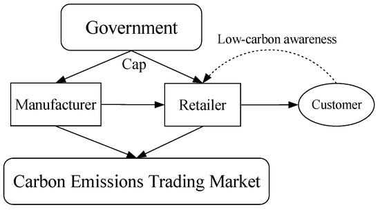
Figure 1.
Concept model.
In order to formulate the mathematical models, some key assumptions are presented as follows.
Assumption 1.
Retailer orders from manufacturer according to demand. No consideration is given to inventory.
Assumption 2.
Potential maximum market demand is fixed.
Assumption 3.
Both production emissions and logistics emissions linearly decrease in quantity [6].
Assumption 4.
Only manufacturer has the ability and opportunity to reduce emissions.
Assumption 5.
Lower production emissions can increase demand.
Moreover, notations that are used in the models are summarized in Table 1.

Table 1.
Notations.
4. Analytical Models
According to the relationship between manufacturer and retailer, two decision-making modes are considered: decentralized and centralized mode. Additionally, the profit-sharing contract is also investigated in this section to fuse these two modes.
4.1. Decentralized Decision-Making Mode
In this subsection, the decentralized decision-making mode is investigated. Under this mode, retailer and manufacturer are independent decision makers. The decision-making process follows the Stackelberg game rule [28]. In this study, the manufacturer is considered as the leader, while the retailer is the follower. In fact, retailer-leading supply chains are widespread, e.g., the Apple Inc.-based supply chain. The retailer determines their selling price to optimize their profit, while the manufacturer supplies them with the product at agreed price . The manufacturer determines carbon-emission reduction level L, which can influence demand since the customer is low-carbon-sensitive. The demand for the product at price and emission-reduction level L for the customer with LCAL h is
Unit cost paid on emission reduction with L is [21]. Here, the quadratic means that, as L grows, the cost increases faster. In other words, investment in emission reduction has a declining marginal effect. Hence, the optimization problem confronted by the manufacturer is formulated as:
where is optimal solution for the following model:
The second items in Equations (2) and (3) are profits from carbon trading by the manufacturer and retailer, respectively. If , the manufacturer (retailer) can profit from selling surplus carbon quotas. On the contrary, the manufacturer (retailer) has to purchase carbon quotas from the trading market to make up for a quota gap when .
The following proposition proposes the optimal decisions under the decentralized decision-making mode.
Proposition 1.
Under the decentralized decision-making mode, let
If , the optimal L, denoted by , is shown in Table 2:
Table 2.
Values of when .
and optimal , denoted by , is
Otherwise, i.e., , the optimal solution is
Proof.
The reverse-solution method for the Stackelberg game was used to solve the problem. For a fixed L determined by the manufacturer, let the first-order derivative of with respect to be zero, i.e.,
which leads to
Plugging in the place of in Equation (2) and the first-order derivative of in L was calculated as
which is a quadratic function of L with discriminant .
If , the two real roots of are denoted as and , respectively. There are two cases based on a comparison of intervals and .
Case 1.. In this case, there are five subcases according to the comparison between and .
Case 1.1.. for any , which indicates that .
Case 1.2.. In order to determine the optimal L, it is necessary to compare with . If is greater than , takes the maximum at ; otherwise, takes the maximum at .
Case 1.3.. increases in L in interval ; hence, takes the maximum at .
Case 1.4.. increases in and decreases in , so takes the maximum at .
Case 1.5.. decreases in , so takes the maximum at .
Case 2.. In this case, there are three subcases according to the comparison between and .
Case 2.1.. Similar to Case 2.1, takes the maximum at .
Case 2.2.. If is greater than , maximizes at ; otherwise, maximizes at .
Case 2.3.. increases in and decreases in , so takes the maximum at .
If for any , which implies that decreases in L. Thus, takes the maximum at .
Plugging in the expression of , is obtained. Thus, this proof is completed. □
Corollary 1.
The manufacturer and retailer’s optimal operation policies ( and ) are independent of allocated caps and .
The corollary is trivial from the expression of and in Proposition 1. Corollary 1 indicates that the allocated caps do not directly influence the optimal decisions. and are influenced by carbon price , which is stated in Corollary 2.
Corollary 2.
Optimal reduction level and retail price increase in if
Proof.
When or 1, is independent of . Next, consider the case that . The first-order derivative of with respect to is . When is not less than , . Combining the expression of , increases in . The monotonicity of in is immediately derived from the expression of . This completes the proof. □
Corollary 2 provides a sufficient condition under which the and increase in . Corollary 2 also implies that higher carbon prices provoke investment in emission-reduction technologies and higher retail prices, which coincides with real practices. This may be explained by the fact that higher carbon prices make emission reductions profitable. At the same time, in order to transfer higher carbon prices to consumers, retailers also set higher retail prices. Although caps do not directly influence optimal decisions of the manufacturer and the retailer, they work by influencing prices. In fact, if generous caps are allocated to firms, decreased carbon prices are inevitable.
Corollary 3.
Optimal reduction level and retail price increase in h if h satisfies
Proof.
When or 1, is independent of h. Since the first-order derivative of in h, rewrite as
where the first item increases in h from , the second item is constant. The first-order derivative of in h is
Inequality leads to and then . In addition,
This completes the proof. □
The values of with different are
and
The changes of with parameters and h are stated by Proposition 2 as follows.
Proposition 2.
(1) linearly increases in ; (2) If the manufacturer has no chance to reduce emissions, their profit increases in when
Meanwhile, is independent of h. (3) If the manufacturer eliminates all emissions, their profit increases in when ; otherwise, decreases in . Meanwhile, increases in h if . (4) increases in when
Meanwhile, increases in h when
Proof.
(1) is derived from the expressions of ; (2), (3), and (4) are derived from solving the inequalities ,, , , and , respectively. □
Similarly, the profits of the retailer with different are calculated as
and
Proposition 3 states the changes of with parameters , , and h.
Proposition 3.
(1) increases in . (2) increases in if . Meanwhile, is independent of h. (3) increases in if . Meanwhile, increases in h if . (4) increases in if . Meanwhile, increases in h if
Proof.
The proof is the same as Proposition 2. □
As emissions are considered, emission amounts from manufacturer and retailer are
and
It is noted that if the manufacturer does not reduce emissions (i.e., ) and has the same emission intensity as the retailer (i.e., ), then emission amounts the manufacturer and retailer are the same. The expressions of and imply that the emission amounts with are independent of caps and . However, and can influence and if and are functions of .
When , and . Both of and increase in and independent of h. This is likely because an increasing inhibits emissions. If the manufacturer eliminates all emissions, i.e., , emissions from the manufacturer are zero. However, emission amount from the retailer is not zero. decreases in but increases in h, which is because increasing carbon prices restrain demand, but increasing LCAL stimulates demand.
The influences of and h on and are stated by Proposition 4.
Proposition 4.
(1) decreases in if
Meanwhile, increases in h if
(2) decreases in if
Meanwhile, increases in h if
Proof.
This proof is derived from solving inequalities and , respectively. □
4.2. Centralized Decision-Making
This subsection focuses on the centralized decision-making mode. When the manufacturer and retailer belong to the same company, they adopt a centralized decision-making mode. Under this mode, the manufacturer and retailer merge into a unified decision maker to optimize the two-stage supply chain. In large-scale companies, this decision-making mode is very common. Under this mode, the allocated emission cap is , and the objective function denoted by is the sum of and proposed in the decentralized decision-making mode, i.e.,
Since , the optimization model for the decision-making problem under the decentralized mode can be formulated by
Optimal solutions for Model (15) are proposed with the following:
Proposition 5.
Proof.
The proof of this proposition is derived from KKT optimality conditions [29]. Then, optimal solution for Problem (15) satisfies KKT optimality conditions, listed as follows:
where
and are Lagrange multipliers.
Multipliers are equal to zero or positive. There are eight possible cases in theory. However, cases with violate feasibility since is strictly greater than zero. Moreover, either and must be zero; otherwise, contradicts with . The remaining three cases may lead to feasible solutions.
Case 1..
It follows from that . The two equations in (18) can be written as
Solving for and in (21) results in
Since , induces .
Case 2..
It follows from that . The former two equations in (18) can be written as
Solving for and in Equation (23) leads to
Assumption leads to , a contradiction.
Case 3..
In this case, the former two equations in (18) can be written as
The second equation in (25) results in
Substituting by (26), the first equation in (25) can be written as
It follows from and that is strictly greater than zero. Thus, the solution of in Equation (27) is
It should be noted that Equation (28) makes practical sense only when . Substituting by Equation (28) in Equation (26) leads to
The second-order derivatives of are calculated as
and
The assumption about a ensures that the following inequalities hold:
where is the determinant of Hessian matrix H with respect to L and . Group of inequalities (33) indicates that is a strictly concave function, which verifies uniqueness. This completes the proof. □
Proposition 5 states that there exist a unique reduction level and retail price to maximize the supply chain’s total profit when the potential maximum market demand a is large enough. Because most firms subject to emission regulation are large-scale and emission-intensive, the assumptions about a in Proposition 5 are reasonable. Proposition 5 also states that optimal reduction level increases in carbon-emission price when is at a low level (). When is greater than , the manufacturer eliminates all emissions, i.e., . That means increasing carbon-emission price is conducive to provoke decision makers to reduce emissions, which coincides with Du et al. [17]. When the price reaches a certain threshold, the incentive effect no longer increases. Here, the threshold is named as critical price and denoted by . Obviously, the critical price increases in k and decreases in h and .
As reduction level and retail price are and respectively, the corresponding profit and emission are
and
where .
The following proposition states the influences of regulation parameters and LCAL on the maximal profit.
Proposition 6.
(1) increases in total emission cap ; (2) When is greater than critical price , decreases in ; otherwise, increases in if , where . (3) When market demand a satisfies the assumption in Proposition 5, increases in h.
Proof.
(1) The conclusion is easily derived from the expression of . (2) When , . Obviously, it decreases in . When , notice that the first-order derivative of in is
so increases in if . (3) This first-order derivative of in h listed as follows:
It follows from assumption about the market demand a that . This completes the proof. □
From Proposition 6, some interesting observations are obtained. When is at a relative low level , profit with respect to varies indefinitely. As is greater than , profit decreases in . Sufficiently high carbon prices prompt the manufacturer to cut all their emissions, i.e., . However, the retailer’s emissions still exist and the retailer pays more with an increasing . Proposition 6(3) implies that the supply chain benefits from a higher LCAL as long as market demand a is big enough.
In order to investigate emission changes with respect to regulation parameters and LCAL, the following is proposed:
Proposition 7.
(1) increases in total emission cap and ; (2) When , decreases in if ; otherwise, decreases in . (3) When , increases in h.
Proof.
(1) The conclusion is trivial from the expression of . (2) When , the first-order derivative of with respect to is
leads to ; When , , which decreases in clearly. (3) When , the conclusion is trivial. When , the conclusion is derived from the first-order derivative of with respect to h:
is equivalent to . This completes the proof. □
Proposition 6(1) and Proposition 7(1) imply that both total profit and emission increase in total cap . The conclusions are easy to understand because the increase of means more relaxed regulations, and more arbitrage and emission opportunities for supply-chain decision makers. It also reminds regulators (governments) that too-loose quotas are not conducive to achieving emission-reduction targets. When , the denominator of is a quadratic function of in Proposition 7(2). If there exist two roots for the quadratic function, only decreases in when lies between the two roots. This means that, if is too low or too high, the increasing results in increasing emissions. When , excessive carbon prices inhibit production and then profit. This suggests that the regulator, who wants to reduce carbon emissions, should control the price within a certain range by setting a reasonable cap. Proposition 7(3) indicates that increasing h does not necessarily result in emission reduction. One possible explanation is that a higher low-carbon premium motivates more production.
4.3. Profit-Sharing Contract
Generally, the decentralized decision-making mode leads to less profit than the centralized decision-making mode due to the effect of double marginalization [30]. To motivate decision makers under the decentralized decision-making mode to make decisions like those in the centralized decision-making mode, one way is to make a profit-sharing contract. As decision makers accept the contract, their decisions change from decentralized to centralized mode. Whether a contract can be executed depends on the proportion of profit being transferred. The following proposition states the range of proportion.
Proposition 8.
Let θ be the proportion of profit shared by the manufacturer. If θ satisfies
both the manufacturer and retailer are willing to accept the profit-sharing contract, where .
Proof.
In order to promote acceptance of the contract by both parties, the profits they obtained from the contract should not be less than the profits they obtained under the decentralized mode, i.e.,
Hence, Equation (36) is easily derived. □
Under the profit-sharing contract, retailer and manufacturer can simultaneously improve their profit levels. The value of represent the retailer/manufacturer’s bargaining power. The smaller means more bargaining power than the manufacturer has. As shown in Equation (36), and are the minimum and maximum that can take. In what follows, they are denoted by and , respectively.
5. Numerical Experiment
In this section, a series of numerical examples are presented to illustrate the theoretical results proposed in this study. As shown in Proposition 1, there are several values under different scenarios. Only some specific scenarios are illustrated in this section, while others can be similarly implemented.
Let . Under this setting, for any positive , where is defined in Proposition 1. In addition, assume that lies in the [1, 10] interval. Thus and , defined in Proposition 1, satisfy . Based on the parameter setting, the influences of on and are shown in Figure 2.
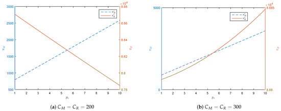
Figure 2.
Influence of on profits under the decentralized decision-making mode.
Figure 2 shows some interesting phenomena. As shown in Figure 2a, both and increase in when . However, increases in when . This is because condition in Proposition 3(3) is not satisfied for any when . Figure 2 indicates that a higher does not necessarily generate more profit with relatively low emission caps. That is likely because relatively low emission caps restrain the space of arbitrage through the carbon-trading market. It should be noted that also decreases in when is less than a threshold.
Let , and . The influence of h on profits is shown in Figure 3. Figure 3 shows that and increase in h. The product obtains more of a low-carbon premium with an increasing h, which means that the consumer is willing to pay more for low-carbon products.
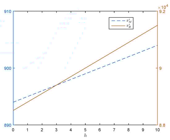
Figure 3.
Influence of h on profits under decentralized decision-making mode.
As stated in Proposition 1, there are several situations for . Let . Under this setting, , implies that . In addition, for any leads to . Profits under the two modes with respect to are illustrated in Figure 4. As shown in Figure 4, the changing trends of and with respect to are different. The curve of is always below curve . This difference exists due to the effect of double marginalization. In order to investigate the influence of h on profits, let and . In this situation, and . The curves of and with respect to h are plotted in Figure 5. As shown in Figure 5, both and increase in h, and always .
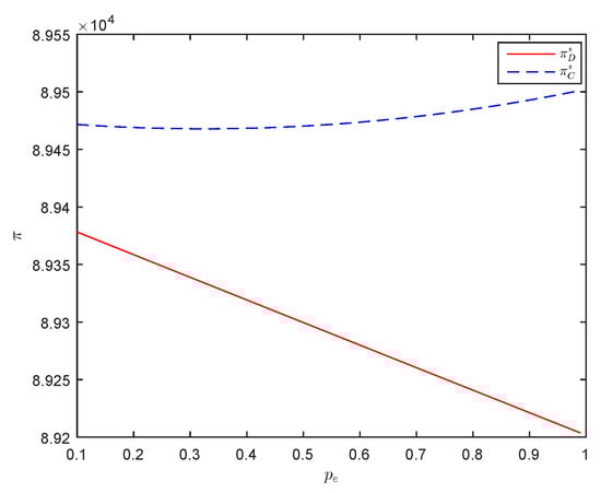
Figure 4.
Influence of on total profits under different modes ().
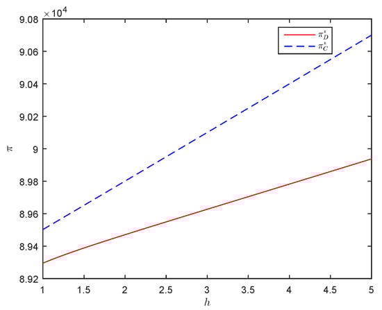
Figure 5.
Influence of h on total profits under different modes.
Let and . It follows from the statement above, and . The curves of and with respect to are plotted in Figure 6. As shown in Figure 6, emissions under both modes decrease in . Emissions under a decentralized mode are always less than emissions under a centralized mode. When and , and . The curves of emissions with respect to h under the two modes are plotted in Figure 7. As shown in Figure 7, both of and decrease in h. Moreover, is greater than for any h. Figure 4, Figure 5, Figure 6 and Figure 7 indicate that the centralized mode dominates the decentralized mode, with higher profits and fewer emissions.
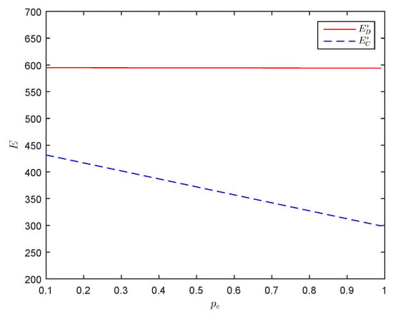
Figure 6.
Influence of on total emissions under different modes ().
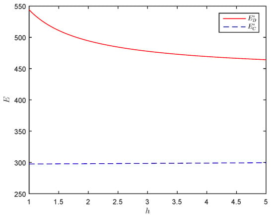
Figure 7.
Influence of h on total emissions under different modes.
At the end of this section, the influence of and h on and is investigated. Since is the feasible interval for , the length of represents the manufacturer’s decision flexibility in profit-sharing mode. Let and . The influence of on and is plotted by Figure 8. Figure 8 shows the distance of , and increases in , which the manufacturer has more decision flexibility with higher under contract mode. Let and , The influence of h on and is plotted by Figure 9. In Figure 9, the distance of and expands with an increasing h. In other words, the manufacturer has more decision flexibility with a higher h.
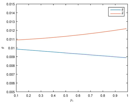
Figure 8.
Influence of on and .
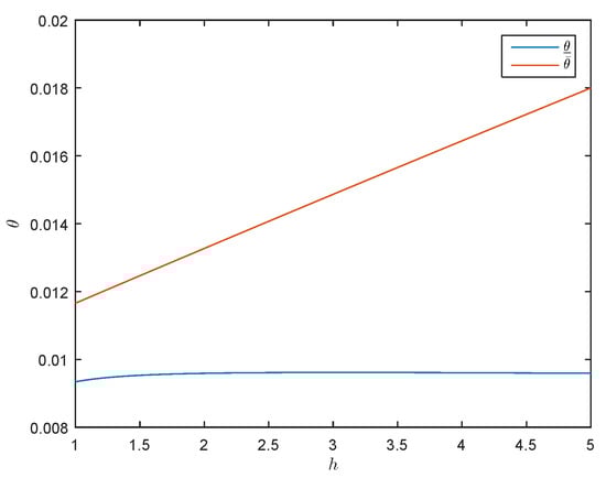
Figure 9.
Influence of h on and .
6. Concluding Remarks and Future Research
This study focused on two-stage supply-chain optimization with carbon-emission consideration. The cap-and-trade regulations and customers’ LCAL were integrated into this problem. The manufacturer decides the emission-reduction level, and the retailer decides the retail price. Considering the different possible relationships between manufacturer and retailer, this study developed two mathematical models for the optimization problem under different decision-making modes (decentralized and centralized modes). The model under the decentralized mode was formulated as a Stackelberg game model and solved by the reverse-solution method. KKT optimality conditions were adopted to deal with the model under the centralized mode. The optimal decisions, corresponding profits, and emissions were derived by solving the models. Several propositions (corollaries) and numerical examples showed the influence of regulation parameters on supply-chain operations. In addition, the profit-sharing contract mode built a bridge between decentralized and centralized mode.
The analytic results and numerical experiments provided some meaningful insights that have realistic significance for regulators and the decision makers in supply chains. First, the optimal solution for decision makers is dependent on parameter settings regardless of decentralized and centralized mode (Propositions 1 and 5). Under a centralized mode, plays an important role in deciding the optimal emission-reduction level when potential demand a is great enough. The cases of an optimal solution under decentralized mode are more complicated. Second, optimal solutions are not influenced by caps allocated by the regulator. However, generous caps lead to more emissions. This reminds the regulator that they should allocate a relatively low cap level. Third, the supply chain can benefit from increasing LCAL from customers. Finally, both higher carbon price and LCAL h can improve manufacturer decision flexibility when there exists a profit-sharing contract.
Compared with existing studies, the contributions of this study are mainly reflected in the following areas: (1) Cap-and-trade regulation and LCAL were integrated in the same supply-chain operation-optimization models; (2) different decision-making modes were introduced in the modelling; (3) the extent to which a manufacturer is willing to transfer profit was investigated when a profit-sharing contract was available. Theoretical results provided meaningful managerial insights for regulators who could control profits and emissions by adjusting regulation parameter settings. For example, if is satisfied, emissions are decreased in (Proposition 4). A regulator can then raise prices by reducing the caps, and the amount of emission reduction can be calculated by theoretical results. In addition, the theoretical results in this study imply that a higher LCAL brings more profits under both modes. Thus, it is beneficial for decision makers of firms if customers’ LCAL is promoted through education and publicity.
Future research can extend this study in the following four aspects. First, there can be more members in the supply chain, rather than only the two in this study. When there are more than one manufacturer or retailer, models are more complex (the Stackelberg–Nash model), and the solution method must be accordingly updated. Second, the study focused on a single-item product-supply chain. How heterogeneous products influence supply-chain operations can be considered in the future. Third, more a precise demand function should be formulated. The demand function affected by LCAL was simplified. The real demand function of LCAL should be derived through statistical techniques, e.g., regression. Fourth, future work should consider the influence of other regulations, such as the carbon tax. Future research expanding from these aspects can help researchers develop more reality-approaching models and provide more managerial insights for regulators and firms.
Funding
This research was funded by the National Natural Science Foundation of China (grant No.71401114), the Fundamental Research Funds for the Central Universities (Sichuan University, Grant No. skqy201524; Business School of Sichuan University, Grant No. B03).
Conflicts of Interest
The author declares no conflict of interest
References
- Diazrainey, I.; Tulloch, D. Carbon pricing and system linking: Lessons from the New Zealand Emissions Trading Scheme. Energy Econ. 2016, 73, 66–79. [Google Scholar] [CrossRef]
- Ranson, M.; Stavins, R. Linkage of Greenhouse Gas Emissions Trading Systems: Learning from Experience. Clim. Policy 2016, 16, 284–300. [Google Scholar] [CrossRef]
- Shammin, R.; Bullard, C. Impact of cap-and-trade policies for reducing greenhouse gas emissions on U.S. households. Ecol. Econ. 2009, 68, 2432–2438. [Google Scholar] [CrossRef]
- Springer, U. The market for tradable GHG permits under the Kyoto Protocol: A survey of model studies. Energy Econ. 2003, 25, 527–551. [Google Scholar] [CrossRef]
- Riahi, K.; Rubin, E.; Taylor, M.; Schrattenholzer, L.; Hounshell, D. Technological learning for carbon capture and sequestration technologies. Energy Econ. 2004, 26, 539–564. [Google Scholar] [CrossRef]
- Benjaafar, S.; Li, Y.; Daskin, M. Carbon Footprint and the Management of Supply Chains: Insights From Simple Models. IEEE Trans. Autom. Sci. Eng. 2013, 1, 99–116. [Google Scholar] [CrossRef]
- Ghosh, D.; Shah, J. Technological learning for carbon capture and sequestration technologies. Int. J. Prod. Econ. 2015, 164, 319–329. [Google Scholar] [CrossRef]
- Yakita, A. Technology choice and environmental awareness in a trade and environment context. Aust. Econ. Pap. 2009, 48, 270–279. [Google Scholar] [CrossRef]
- Liu, T.; Wang, Q.; Su, B. A review of carbon labeling: Standards, implementation, and impact. Renew. Sustain. Energy Rev. 2016, 53, 68–79. [Google Scholar] [CrossRef]
- Millardball, A. Cap-and-Trade: Five Implications for Transportation Planners. Energy Policy 2009, 2119, 20–26. [Google Scholar]
- Hua, G.; Cheng, T.; Wang, S. Managing carbon footprints in inventory management. Int. J. Prod. Econ. 2011, 2, 178–185. [Google Scholar] [CrossRef]
- Chen, X.; Benjaafar, S.; Elomri, A. The carbon-constrained EOQ. Oper. Res. Lett. 2013, 41, 142–149. [Google Scholar] [CrossRef]
- Tao, Z.; Xu, J. Carbon-Regulated EOQ Models with Consumers’ Low-Carbon Awareness. Sustainability 2019, 4, 4626. [Google Scholar] [CrossRef]
- Toptal, A.; Ozlu, H.; Konur, D. Joint decisions on inventory replenishment and emission reduction investment under different emission regulations. Int. J. Prod. Res. 2014, 52, 243–269. [Google Scholar] [CrossRef]
- Du, S.; Hu, L.; Song, M. Production optimization considering environmental performance and preference in the cap-and-trade system. J. Clean. Prod. 2016, 112, 1600–1607. [Google Scholar] [CrossRef]
- Zhang, B.; Xu, L. Multi-item production planning with carbon cap and trade mechanism. Int. J. Prod. Econ. 2013, 1, 118–127. [Google Scholar] [CrossRef]
- Du, S.; Tang, W.; Song, M. Low-carbon production with low-carbon premium in cap-and-trade regulation. Int. J. Prod. J. Clean. Prod. 2016, 134, 652–662. [Google Scholar] [CrossRef]
- Du, S.; Fu, Z.; Zhu, L.; Zhang, J. Game-theoretic analysis for an emission-dependent supply chain in a ‘cap-and-trade’ system. Ann. Oper. Res. 2015, 1, 135–149. [Google Scholar] [CrossRef]
- Xu, X.; Zhang, W.; He, P.; Xu, X. Production and pricing problems in make-to-order supply chain with cap-and-trade regulation. Omega-Int. J. Manag. S 2017, 66, 248–257. [Google Scholar] [CrossRef]
- Xu, L.; Wang, C.; Zhao, J. Decision and coordination in the dual-channel supply chain considering cap-and-trade regulation. J. Clean. Prod. 2018, 197, 551–561. [Google Scholar] [CrossRef]
- Liu, Z.; Anderson, T.; Cruz, J. Consumer environmental awareness and competition in two-stage supply chains. Eur. J. Oper. Res. 2012, 3, 602–613. [Google Scholar] [CrossRef]
- Xia, L.; Hao, W.; Qin, J.; Ji, F.; Yue, X. Carbon emission reduction and promotion policies considering social preferences and consumers’ low-carbon awareness in the cap-and-trade system. J. Clean. Prod. 2018, 195, 1105–1124. [Google Scholar] [CrossRef]
- Shuai, C.; Ding, L.; Zhang, Y.; Guo, Q.; Shuai, J. How consumers are willing to pay for low-carbon products?-Results from a carbon-labeling scenario experiment in China. J. Clean. Prod. 2014, 83, 366–373. [Google Scholar] [CrossRef]
- Zhao, R.; Geng, Y.; Liu, Y.; Tao, X.; Xue, B. Consumers’ perception, purchase intention, and willingness to pay for carbon-labeled products: A case study of Chengdu in China. J. Clean. Prod. 2018, 171, 1664–1671. [Google Scholar] [CrossRef]
- Conrad, K. Price competition and product differentiation when consumers care for the environment. Environ. Resour. Econ. 2005, 1, 1–19. [Google Scholar] [CrossRef]
- Ji, J.; Zhang, Z.; Yang, L. Carbon emission reduction decisions in the retail-/dual-channel supply chain with consumers’ preference. J. Clean. Prod. 2017, 141, 852–867. [Google Scholar] [CrossRef]
- Wang, L.; Xu, T.; Qin, L. A Study on Supply Chain Emission Reduction Level Based on Carbon Tax and Consumers’ Low-Carbon Preferences under Stochastic Demand. Math. Probl. Eng. 2019, 2019, 1–20. [Google Scholar] [CrossRef]
- Yu, Y.; Huang, G.; Liang, L. Stackelberg game-theoretic model for optimizing advertising, pricing and inventory policies in vendor managed inventory (VMI) production supply chains. Comput. Ind. Eng. 2009, 1, 368–382. [Google Scholar] [CrossRef]
- Boyd, S.; Vandenberghe, L. Optimality conditions. In Convex Optimization; Cambridge University Press: New York, NY, USA, 2004; pp. 241–249. [Google Scholar]
- Jamali, M.; Rastibarzoki, M. A game theoretic approach for green and non-green product pricing in chain-to-chain competitive sustainable and regular dual-channel supply chains. J. Clean. Prod. 2018, 170, 1029–1043. [Google Scholar] [CrossRef]
© 2019 by the author. Licensee MDPI, Basel, Switzerland. This article is an open access article distributed under the terms and conditions of the Creative Commons Attribution (CC BY) license (http://creativecommons.org/licenses/by/4.0/).