Green Façade Effects on Thermal Environment in Transitional Space: Field Measurement Studies and Computational Fluid Dynamics Simulations


Abstract
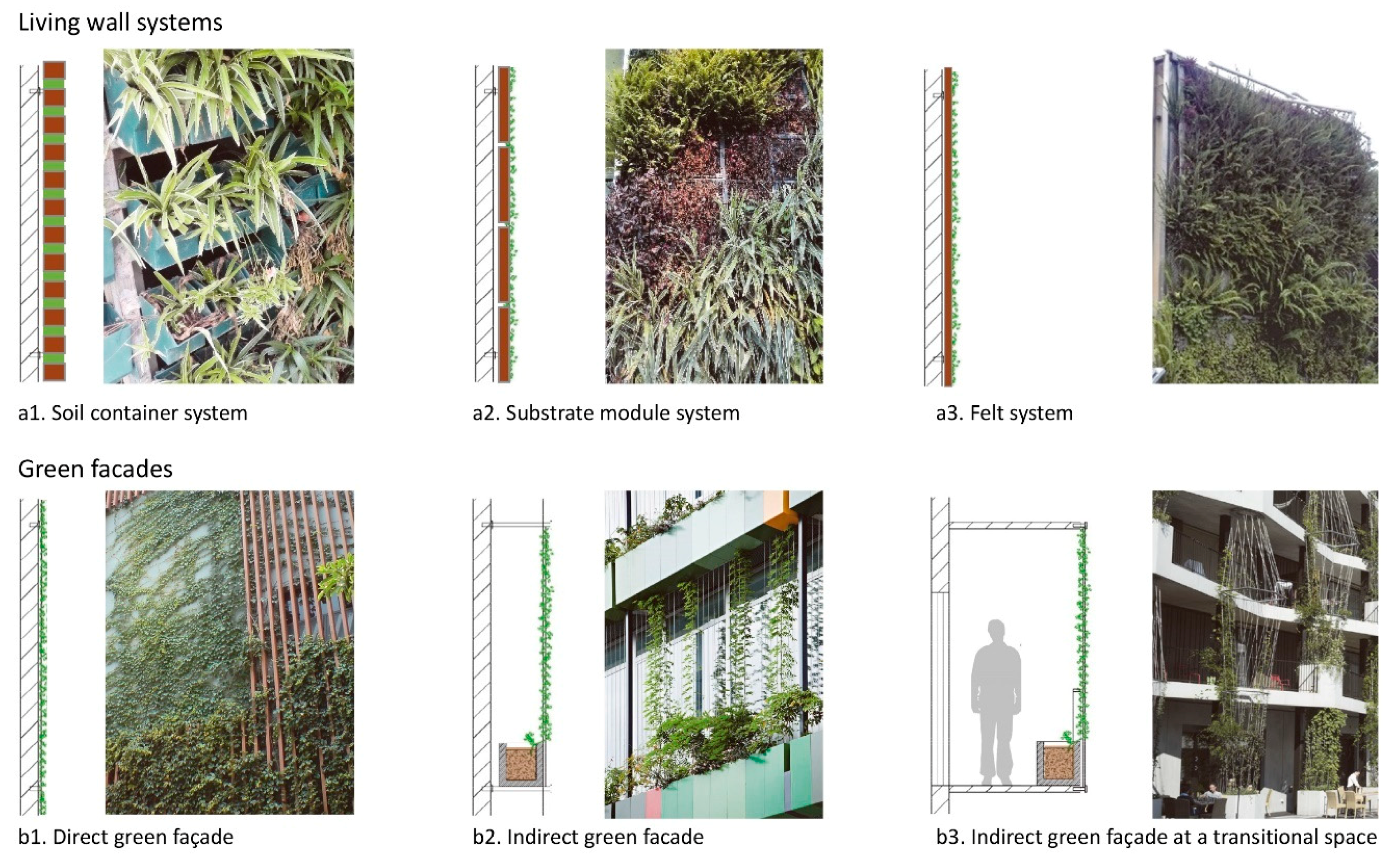
1. Introduction
2. Methodology
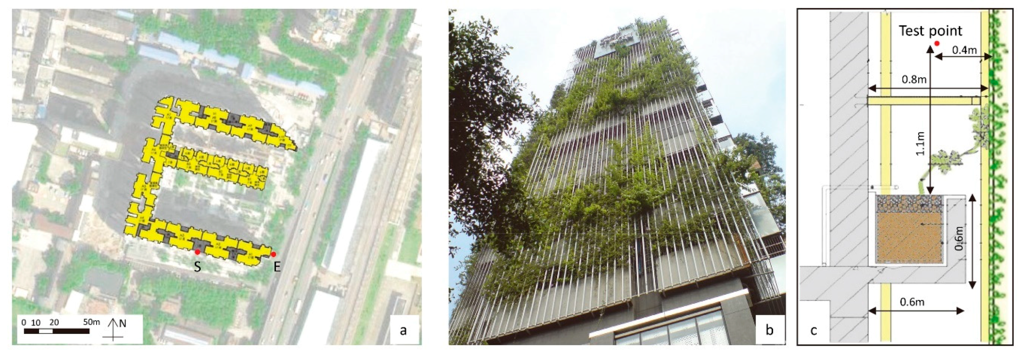
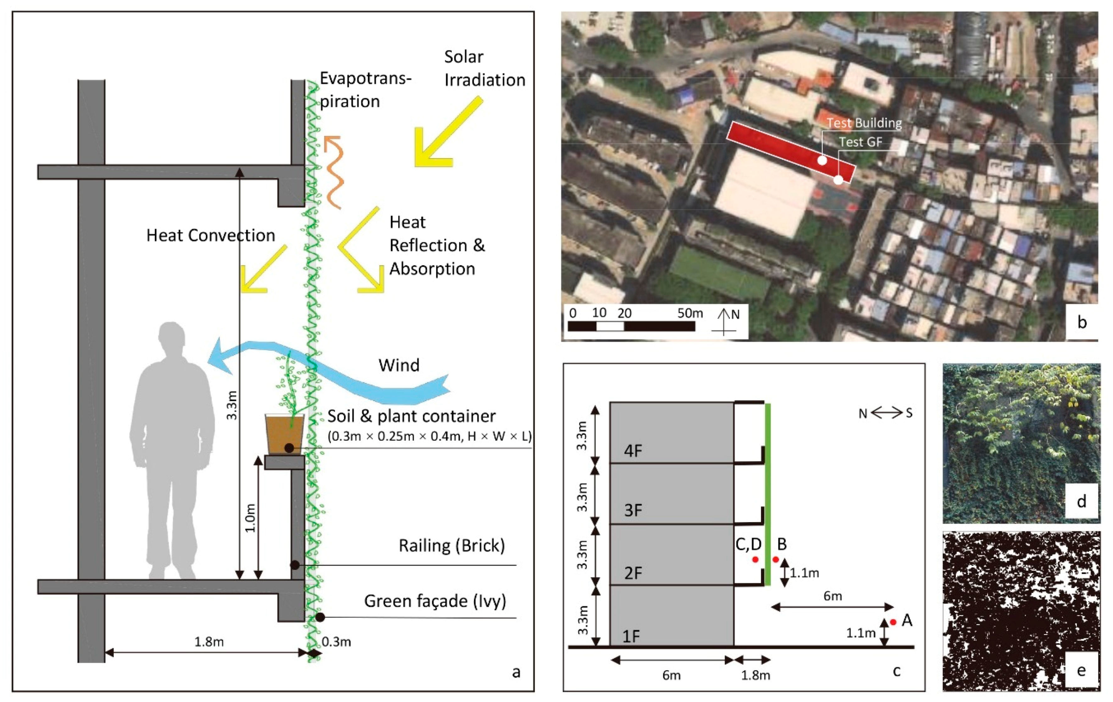
2.1. Setting of Field Measurements
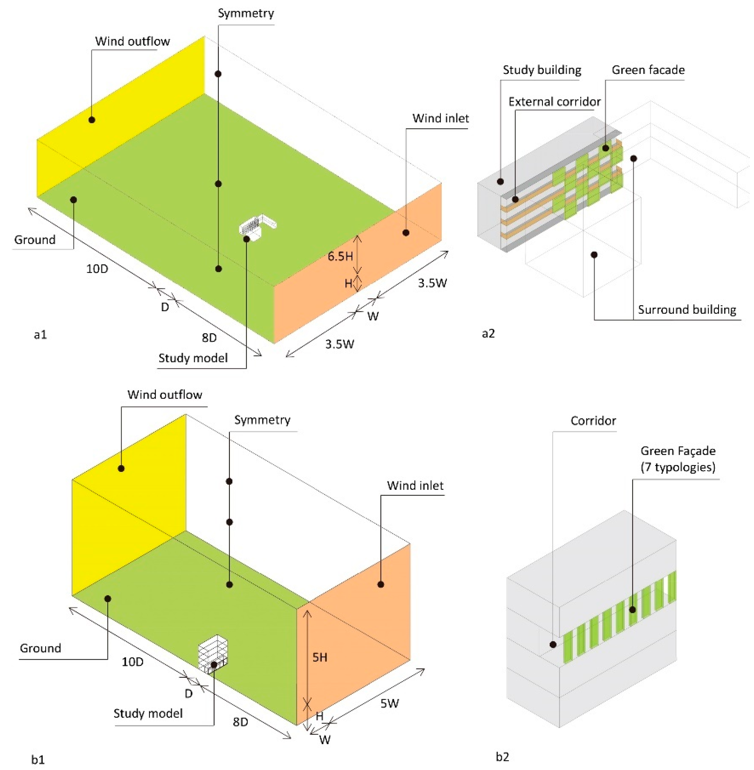
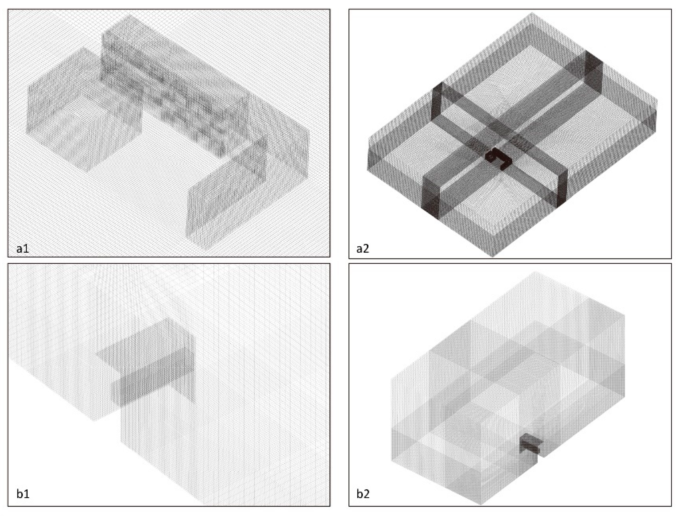
2.2. Base Settings of CFD Simulation
2.3. Definition of GF in the CFD Model
2.4. Physical Parameters Calculated in the CFD Model
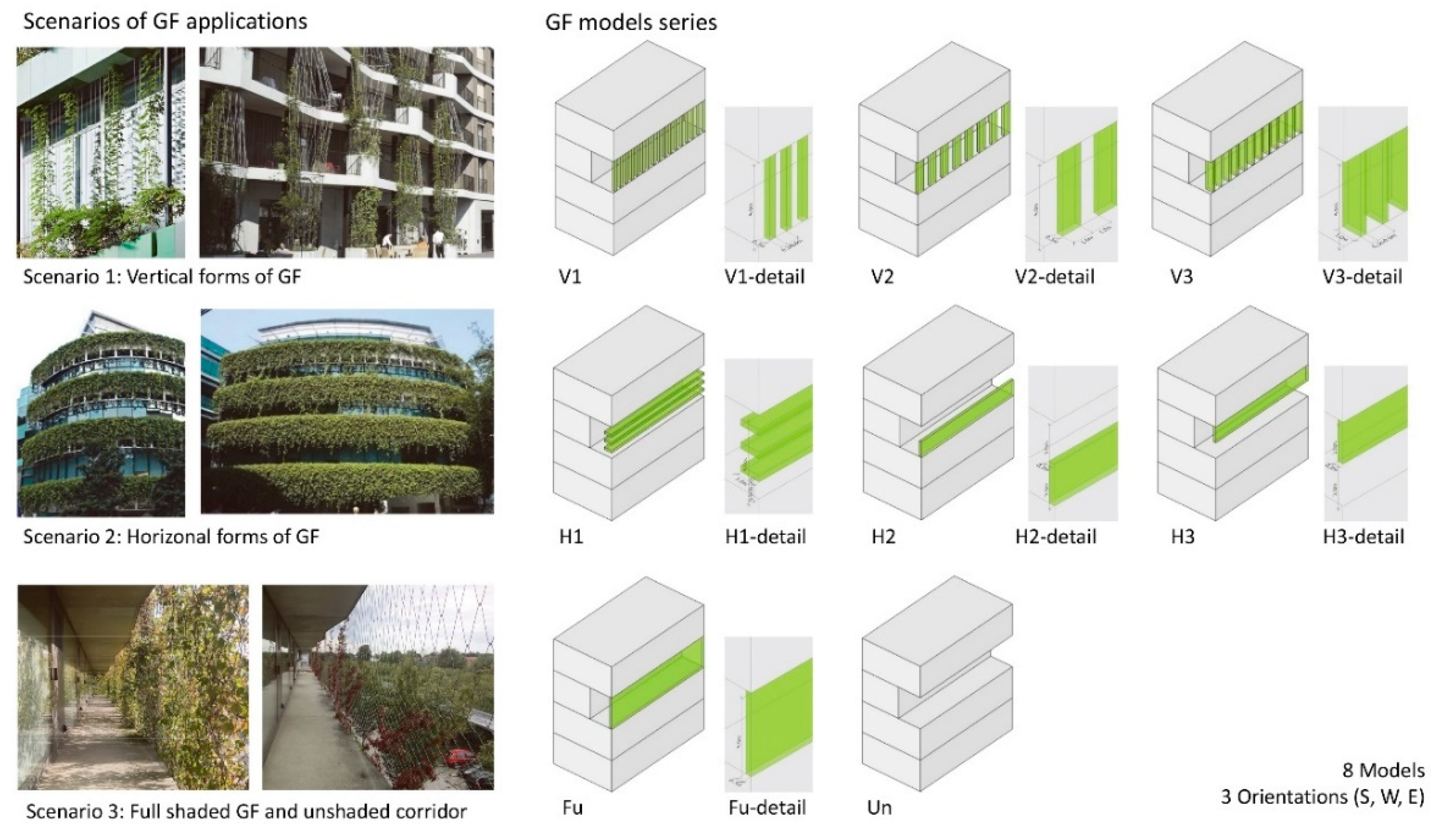
2.5. GF Typologies Models
3. Results
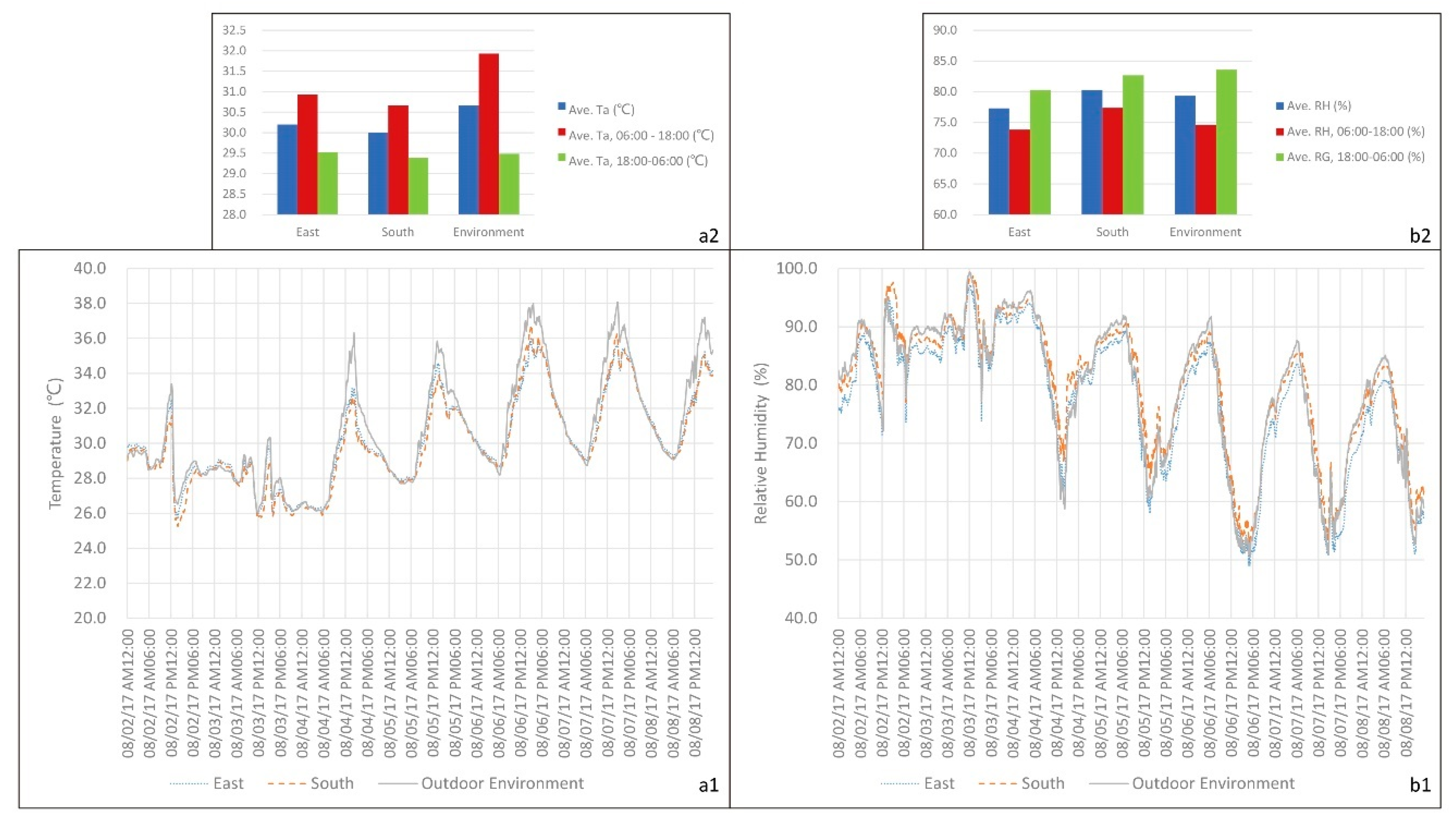
3.1. Field Measurement Results
3.1.1. Field Measurement A
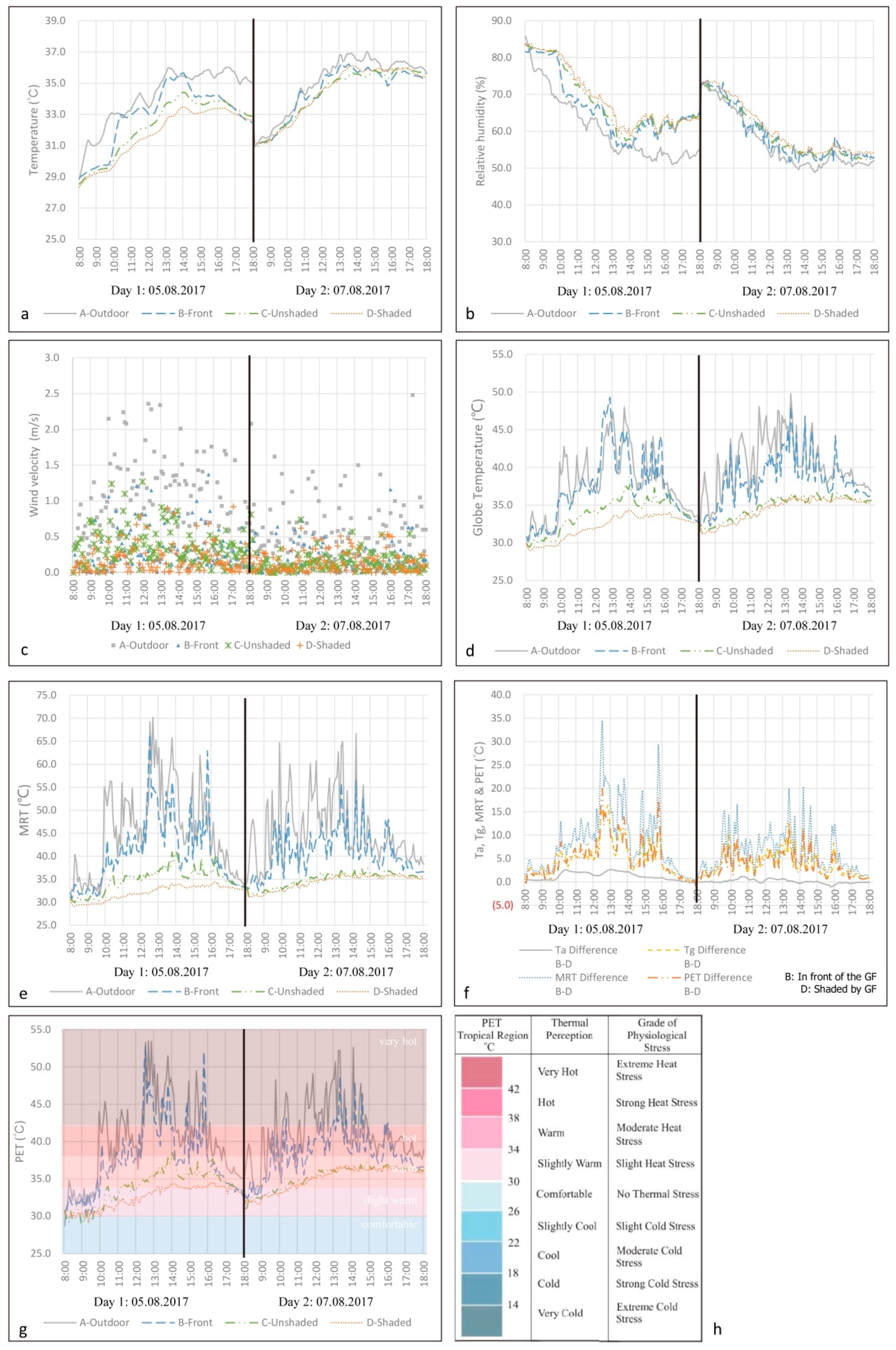
3.1.2. Field Measurement B
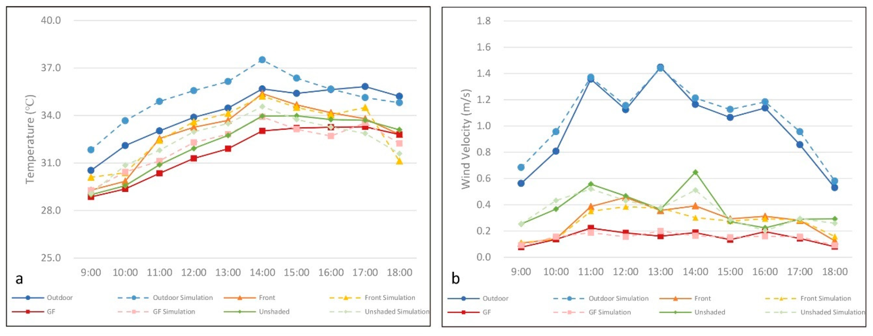
3.2. Validation of Simulation
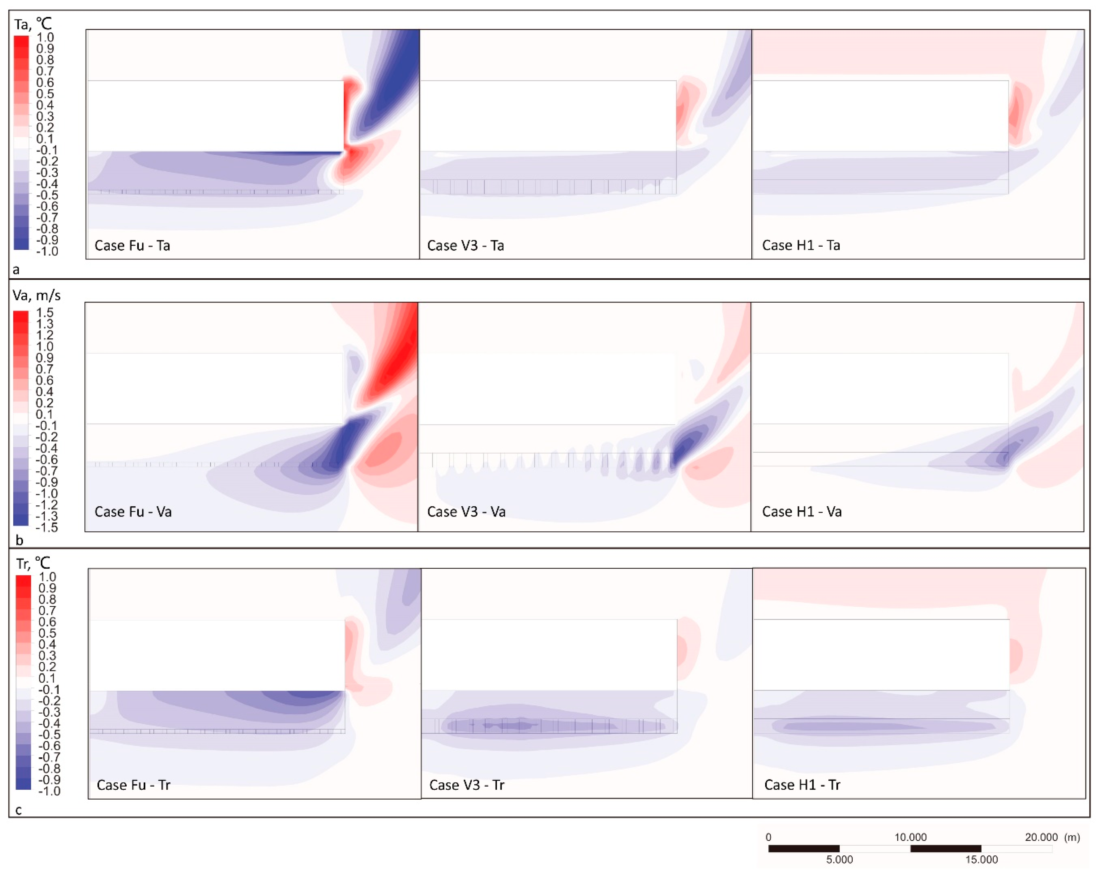
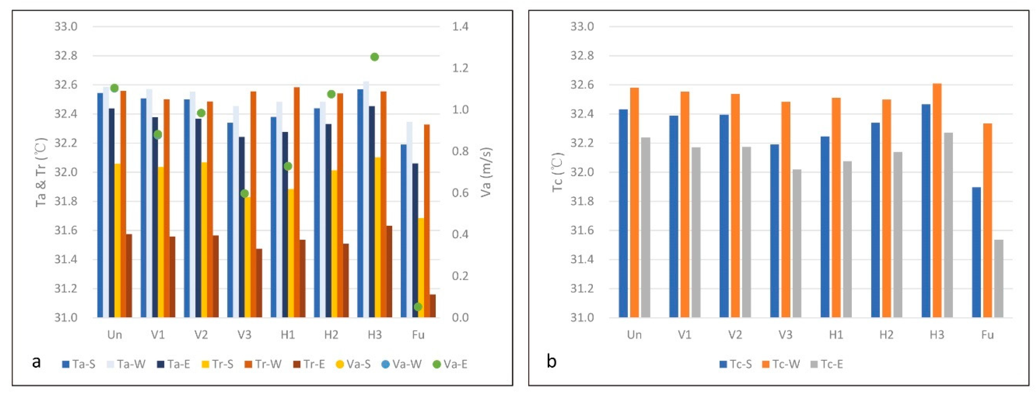
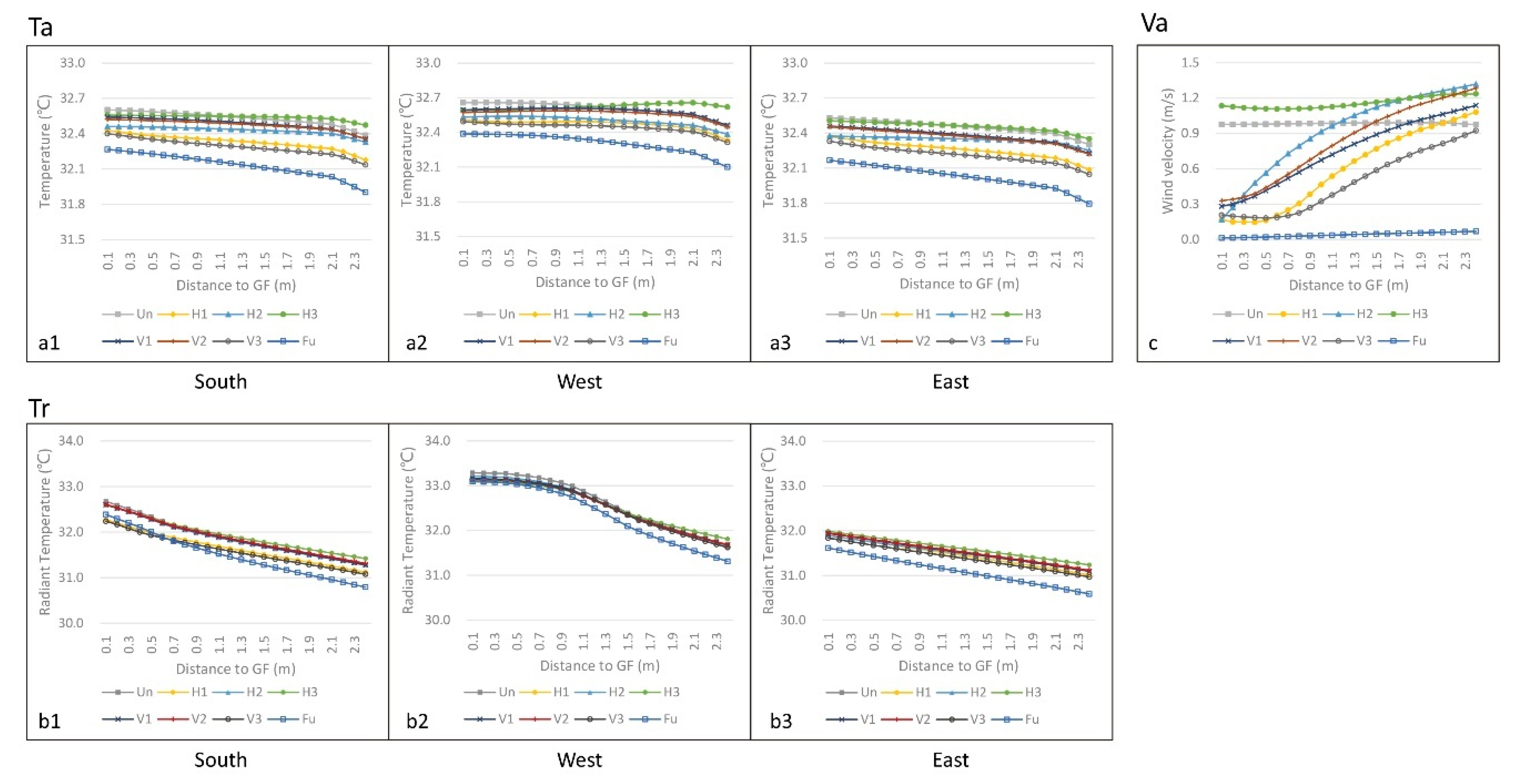
3.3. Results of GF Typologies
4. Discussion
4.1. Thermal Comfort in Field Measurements
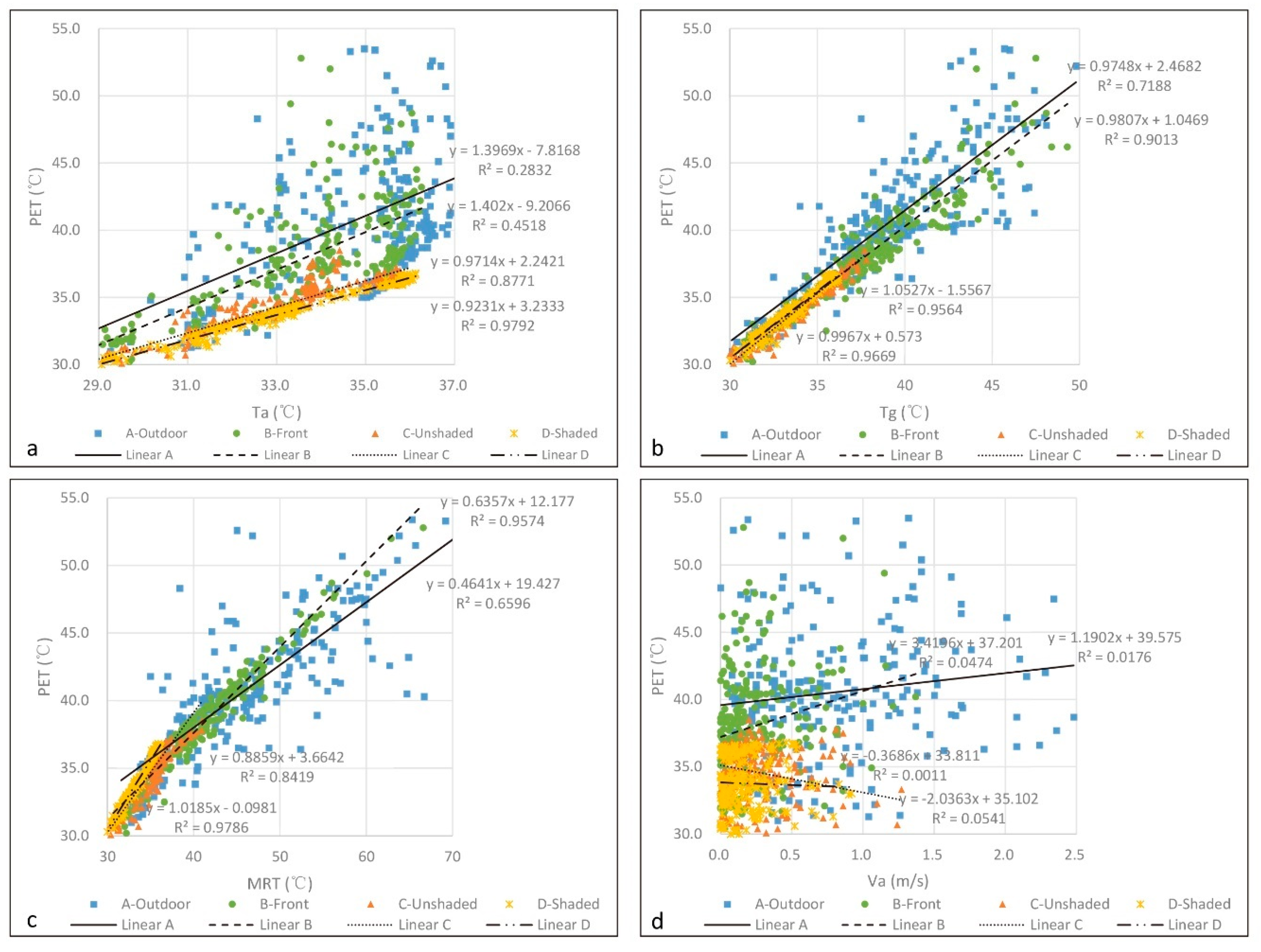
4.2. Correlation Analysis of Indices with PET
4.3. Analysis of GF Shading Effect
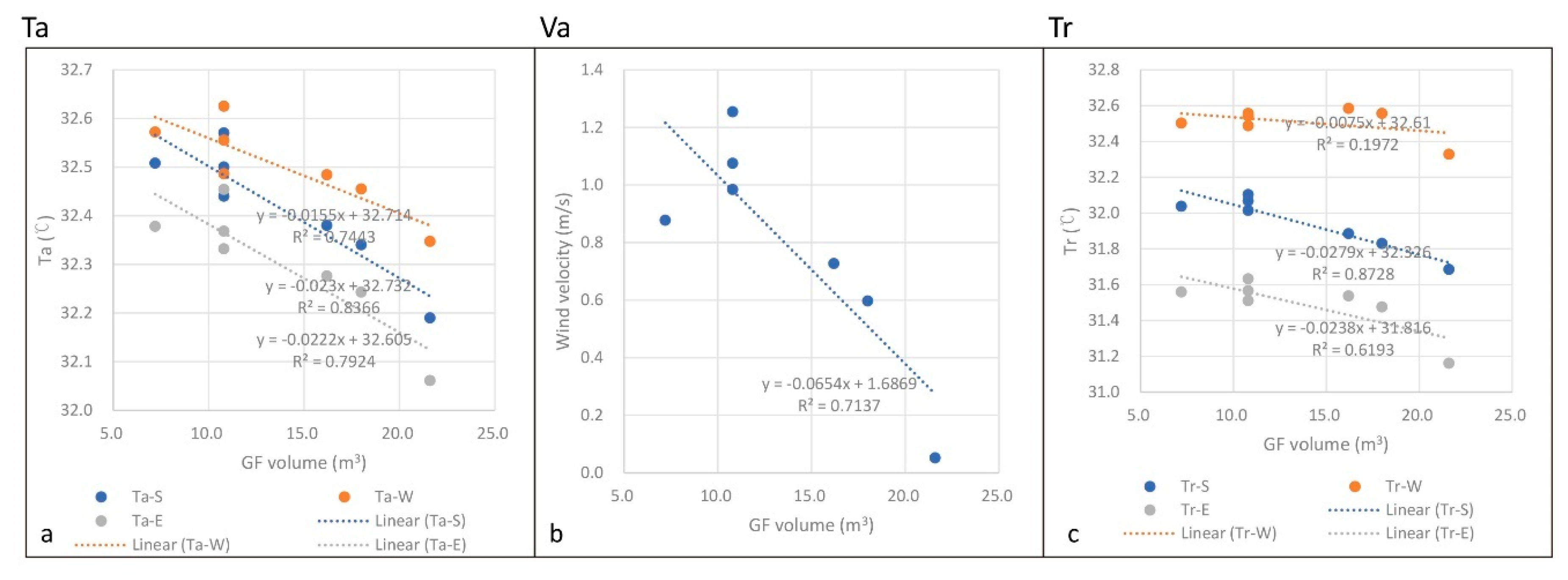
4.4. GF Volume and Its Effect on Thermal Comfort
4.5. Limitations of This Study
5. Conclusions
Author Contributions
Funding
Acknowledgments
Conflicts of Interest
Appendix A

| Indices | A: Outdoor | B: Front | C: Unshaded | D: Shaded | Difference A–B | Difference A–D | Difference C–D |
|---|---|---|---|---|---|---|---|
| Ta (°C) | |||||||
| Day1 Ave. | 34.23 | 32.98 | 32.30 | 31.77 | 1.25 | 2.46 | 0.53 |
| Day1 Max. | 36.01 | 35.66 | 34.41 | 33.47 | 0.35 | 2.54 | 0.94 |
| Day1 Min. | 29.27 | 29.02 | 28.62 | 28.47 | 0.25 | 0.80 | 0.15 |
| Day2 Ave. | 34.99 | 34.47 | 34.31 | 34.37 | 0.52 | 0.62 | −0.06 |
| Day2 Max. | 36.01 | 35.66 | 34.41 | 33.47 | 0.35 | 2.54 | 0.94 |
| Day2 Min. | 30.85 | 31.13 | 30.93 | 31.15 | −0.28 | −0.30 | −0.23 |
| RH (%) | |||||||
| Day1 Ave. | 60.79 | 66.53 | 68.20 | 69.21 | −5.74 | −8.42 | −1.00 |
| Day1 Max. | 84.29 | 82.43 | 83.31 | 83.70 | 1.87 | 0.59 | −0.39 |
| Day1 Min. | 50.94 | 55.31 | 57.44 | 58.56 | −4.37 | −7.62 | −1.12 |
| Day2 Ave. | 57.11 | 59.09 | 59.38 | 60.60 | −1.98 | −3.48 | −1.22 |
| Day2 Max. | 73.23 | 74.25 | 73.01 | 73.95 | −1.02 | −0.72 | −0.94 |
| Day2 Min. | 48.80 | 51.39 | 52.25 | 53.35 | −2.59 | −4.55 | −1.11 |
| Va (m s−1) | |||||||
| Day1 Ave. | 1.01 | 0.32 | 0.37 | 0.19 | 0.68 | 0.81 | 0.18 |
| Day1 Max. | 2.36 | 1.37 | 1.27 | 0.92 | 0.99 | 1.44 | 0.35 |
| Day1 Min. | 0.07 | 0.00 | 0.01 | 0.00 | 0.07 | 0.07 | 0.01 |
| Day2 Ave. | 0.55 | 0.18 | 0.16 | 0.16 | 0.37 | 0.39 | 0.00 |
| Day2 Max. | 2.48 | 1.16 | 0.81 | 0.62 | 1.32 | 1.86 | 0.19 |
| Day2 Min. | 0.00 | 0.00 | 0.00 | 0.00 | 0.00 | 0.00 | 0.00 |
| Tg (°C) | |||||||
| Day1 Ave. | 37.76 | 37.18 | 33.87 | 32.15 | 0.58 | 5.61 | 1.73 |
| Day1 Max. | 48.00 | 49.30 | 37.80 | 34.30 | −1.30 | 13.70 | 3.50 |
| Day1 Min. | 30.10 | 30.30 | 29.40 | 29.00 | −0.20 | 1.10 | 0.40 |
| Day2 Ave. | 40.32 | 38.34 | 34.81 | 34.44 | 1.98 | 5.88 | 0.37 |
| Day2 Max. | 49.80 | 48.10 | 36.70 | 36.20 | 1.70 | 13.60 | 0.50 |
| Day2 Min. | 32.50 | 32.20 | 31.20 | 31.20 | 0.30 | 1.30 | 0.00 |
| MRT (°C) | |||||||
| Day1 Ave. | 45.27 | 40.68 | 34.83 | 32.09 | 4.59 | 13.18 | 2.74 |
| Day1 Max. | 70.20 | 66.60 | 41.00 | 34.40 | 3.60 | 35.80 | 6.60 |
| Day1 Min. | 31.60 | 30.70 | 29.90 | 29.10 | 0.90 | 2.50 | 0.80 |
| Day2 Ave. | 45.52 | 40.71 | 34.95 | 34.37 | 4.81 | 11.15 | 0.58 |
| Day2 Max. | 70.20 | 66.60 | 41.00 | 34.40 | 3.60 | 35.80 | 6.60 |
| Day2 Min. | 33.90 | 32.50 | 31.30 | 31.10 | 1.40 | 2.80 | 0.20 |
| PET (°C) | |||||||
| Day1 Ave. | 40.21 | 37.79 | 34.01 | 32.58 | 2.42 | 7.63 | 1.43 |
| Day1 Max. | 53.50 | 52.80 | 38.50 | 34.50 | 0.70 | 19.00 | 4.00 |
| Day1 Min. | 31.30 | 30.20 | 29.00 | 29.10 | 1.10 | 2.20 | −0.10 |
| Day2 Ave. | 41.02 | 38.48 | 35.25 | 34.98 | 2.54 | 6.04 | 0.27 |
| Day2 Max. | 52.60 | 48.70 | 37.20 | 36.80 | 3.90 | 15.80 | 0.40 |
| Day2 Min. | 31.60 | 32.30 | 30.70 | 31.50 | −0.70 | 0.10 | −0.80 |
References
- Zölch, T.; Maderspacher, J.; Wamsler, C.; Pauleit, S. Using Green Infrastructure for Urban Climate-Proofing: An Evaluation of Heat Mitigation Measures at the Micro-Scale. Urban For. Urban Green. 2016, 20, 305–316. [Google Scholar] [CrossRef]
- Pérez, G.; Coma, J.; Martorell, I.; Cabeza, L.F. Vertical Greenery Systems (VGS) for Energy Saving in Buildings: A Review. Renew. Sustain. Energy Rev. 2014, 39, 139–165. [Google Scholar] [CrossRef]
- de Jesus, M.P.; Lourenço, J.M.; Arce, R.M.; Macias, M. Green Façades and in Situ Measurements of Outdoor Building Thermal Behaviour. Build. Environ. 2017, 119, 11–19. [Google Scholar] [CrossRef]
- Manso, M.; Castro-Gomes, J. Green Wall Systems: A Review of Their Characteristics. Renew. Sustain. Energy Rev. 2015, 41, 863–871. [Google Scholar] [CrossRef]
- Jim, C.Y. Greenwall Classification and Critical Design-Management Assessments. Ecol. Eng. 2015, 77, 348–362. [Google Scholar] [CrossRef]
- Growing Green Guide. Available online: http://www.growinggreenguide.org/wp-content/uploads/2014/02/growing_green_guide_ebook_130214.pdf (accessed on 10 October 2019).
- Johnston, J.; Newton, J. Greater London Authority. Building Green: A Guide to Using Plants on Roofs, Walls and Pavements; Greater London Authority: London, UK, 2004. [Google Scholar]
- Helzel, M. World Stainless. Available online: http://www.worldstainless.org/Files/issf/non-image-files/PDF/Euro_Inox/VertGardens_EN.pdf (accessed on 11 October 2019).
- Chew, M.Y.L.; Conejos, S.; Azril, F.H.B. Design for Maintainability of High-Rise Vertical Green Facades. Build. Res. Inf. 2019, 47, 453–467. [Google Scholar] [CrossRef]
- Perini, K.; Rosasco, P. Cost–Benefit Analysis for Green Façades and Living Wall Systems. Build. Environ. 2013, 70, 110–121. [Google Scholar] [CrossRef]
- Wong, N.H.; Kwang Tan, A.Y.; Chen, Y.; Sekar, K.; Tan, P.Y.; Chan, D.; Chiang, K.; Wong, N.C. Thermal Evaluation of Vertical Greenery Systems for Building Walls. Build. Environ. 2010, 45, 663–672. [Google Scholar] [CrossRef]
- Köppen, W. The Thermal Zones of the Earth According to the Duration of Hot, Moderate and Cold Periods and to the Impact of Heat on the Organic World. Metz 2011, 20, 351–360. [Google Scholar] [CrossRef]
- Sunakorn, P.; Yimprayoon, C. Thermal Performance of Biofacade with Natural Ventilation in the Tropical Climate. Procedia Eng. 2011, 21, 34–41. [Google Scholar] [CrossRef]
- Jim, C.Y. Cold-Season Solar Input and Ambivalent Thermal Behavior Brought by Climber Greenwalls. Energy 2015, 90, 926–938. [Google Scholar] [CrossRef]
- Kontoleon, K.J.; Eumorfopoulou, E.A. The Effect of the Orientation and Proportion of a Plant-Covered Wall Layer on the Thermal Performance of a Building Zone. Build. Environ. 2010, 45, 1287–1303. [Google Scholar] [CrossRef]
- Coma, J.; Pérez, G.; de Gracia, A.; Burés, S.; Urrestarazu, M.; Cabeza, L.F. Vertical Greenery Systems for Energy Savings in Buildings: A Comparative Study between Green Walls and Green Facades. Build. Environ. 2017, 111, 228–237. [Google Scholar] [CrossRef]
- Perini, K.; Ottelé, M.; Fraaij, A.L.A.; Haas, E.M.; Raiteri, R. Vertical Greening Systems and the Effect on Air Flow and Temperature on the Building Envelope. Build. Environ. 2011, 46, 2287–2294. [Google Scholar] [CrossRef]
- Koyama, T.; Yoshinaga, M.; Maeda, K.; Yamauchi, A. Transpiration Cooling Effect of Climber Greenwall with an Air Gap on Indoor Thermal Environment. Ecol. Eng. 2015, 83, 343–353. [Google Scholar] [CrossRef]
- Jim, C.Y.; He, H. Estimating Heat Flux Transmission of Vertical Greenery Ecosystem. Ecol. Eng. 2011, 37, 1112–1122. [Google Scholar] [CrossRef]
- Pérez, G.; Rincón, L.; Vila, A.; González, J.M.; Cabeza, L.F. Behaviour of Green Facades in Mediterranean Continental Climate. Energy Convers. Manag. 2011, 52, 1861–1867. [Google Scholar] [CrossRef]
- Flores Larsen, S.; Filippín, C.; Lesino, G. Modeling Double Skin Green Façades with Traditional Thermal Simulation Software. Sol. Energy 2015, 121, 56–67. [Google Scholar] [CrossRef]
- Tan, C.L.; Wong, N.H.; Tan, P.Y.; Jusuf, S.K.; Chiam, Z.Q. Impact of Plant Evapotranspiration Rate and Shrub Albedo on Temperature Reduction in the Tropical Outdoor Environment. Build. Environ. 2015, 94, 206–217. [Google Scholar] [CrossRef]
- Šuklje, T.; Medved, S.; Arkar, C. On Detailed Thermal Response Modeling of Vertical Greenery Systems as Cooling Measure for Buildings and Cities in Summer Conditions. Energy 2016, 115, 1055–1068. [Google Scholar] [CrossRef]
- Šuklje, T.; Arkar, C.; Medved, S. The Local Ventilation System Coupled with the Indirect Green Façade: A Priliminary Study. Int. J. Des. Nat. Ecodyn. 2014, 9, 314–320. [Google Scholar] [CrossRef]
- Chun, C.; Kwok, A.; Tamura, A. Thermal Comfort in Transitional Spaces–Basic Concepts: Literature Review and Trial Measurement. Build. Env. 2004, 39, 1187–1192. [Google Scholar] [CrossRef]
- Chun, C.; Tamura, A. Thermal Comfort in Urban Transitional Spaces. Build. Env. 2005, 40, 633–639. [Google Scholar] [CrossRef]
- China Meteorological Administration (In Chinese). Available online: http://www.cma.gov.cn/en2014/ (accessed on 11 October 2019).
- Bellia, L.; Marino, C.; Minichiello, F.; Pedace, A. An Overview on Solar Shading Systems for Buildings. Energy Procedia 2014, 62, 309–317. [Google Scholar] [CrossRef]
- Mirrahimi, S.; Mohamed, M.F.; Haw, L.C.; Ibrahim, N.L.N.; Yusoff, W.F.M.; Aflaki, A. The Effect of Building Envelope on the Thermal Comfort and Energy Saving for High-Rise Buildings in Hot–Humid Climate. Renew. Sustain. Energy Rev. 2016, 53, 1508–1519. [Google Scholar] [CrossRef]
- Zhang, Z.; Zhang, Y.; Ding, E. Acceptable Temperature Steps for Transitional Spaces in the Hot-Humid Area of China. Build. Environ. 2017, 121, 190–199. [Google Scholar] [CrossRef]
- Jitkhajornwanich, K.; Pitts, A.C. Interpretation of Thermal Responses of Four Subject Groups in Transitional Spaces of Buildings in Bangkok. Build. Environ. 2002, 37, 1193–1204. [Google Scholar] [CrossRef]
- Toparlar, Y.; Blocken, B.; Maiheu, B.; van Heijst, G.J.F. A Review on the CFD Analysis of Urban Microclimate. Renew. Sustain. Energy Rev. 2017, 80, 1613–1640. [Google Scholar] [CrossRef]
- Lin, H.; Xiao, Y.; Musso, F. Shading Effect and Heat Reflection Performance of Green Façade in Hot Humid Climate Area: Measurements of a Residential Project in Guangzhou, China. IOP Conf. Ser. Earth Environ. Sci. 2018, 146, 012006. [Google Scholar] [CrossRef]
- International Organization for Standardization. Available online: https://www.iso.org/standard/14561.html (accessed on 11 October 2019).
- Mayer, H.; Höppe, P. Thermal Comfort of Man in Different Urban Environments. Theor. Appl. Climatol. 1987, 38, 43–49. [Google Scholar] [CrossRef]
- Matzarakis, A.; Rutz, F.; Mayer, H. Modelling Radiation Fluxes in Simple and Complex Environments—Application of the RayMan Model. Int. J. Biometeorol 2007, 51, 323–334. [Google Scholar] [CrossRef] [PubMed]
- Ip, K.; Lam, M.; Miller, A. Shading Performance of a Vertical Deciduous Climbing Plant Canopy. Build. Environ. 2010, 45, 81–88. [Google Scholar] [CrossRef]
- Koyama, T.; Yoshinaga, M.; Hayashi, H.; Maeda, K.; Yamauchi, A. Identification of Key Plant Traits Contributing to the Cooling Effects of Green Façades Using Freestanding Walls. Build. Environ. 2013, 66, 96–103. [Google Scholar] [CrossRef]
- Gromke, C.; Blocken, B.; Janssen, W.; Merema, B.; van Hooff, T.; Timmermans, H. CFD Analysis of Transpirational Cooling by Vegetation: Case Study for Specific Meteorological Conditions during a Heat Wave in Arnhem, Netherlands. Build. Environ. 2015, 83, 11–26. [Google Scholar] [CrossRef]
- Shih, T.-H.; Liou, W.W.; Shabbir, A.; Yang, Z.; Zhu, J. A New K-ϵ Eddy Viscosity Model for High Reynolds Number Turbulent Flows. Comput. Fluids 1995, 24, 227–238. [Google Scholar] [CrossRef]
- Fidaros, D.K.; Baxevanou, C.A.; Bartzanas, T.; Kittas, C. Numerical Simulation of Thermal Behavior of a Ventilated Arc Greenhouse during a Solar Day. Renew. Energy 2010, 35, 1380–1386. [Google Scholar] [CrossRef]
- Richards, P.J.; Hoxey, R.P. Appropriate Boundary Conditions for Computational Wind Engineering Models Using the K-ϵ Turbulence Model. J. Wind Eng. Ind. Aerodyn. 1993, 46–47, 145–153. [Google Scholar] [CrossRef]
- López, A.; Molina-Aiz, F.D.; Valera, D.L.; Peña, A. Determining the Emissivity of the Leaves of Nine Horticultural Crops by Means of Infrared Thermography. Sci. Hortic. 2012, 137, 49–58. [Google Scholar] [CrossRef]
- Mercer, G.N. Modelling to Determine the Optimal Porosity of Shelterbelts for the Capture of Agricultural Spray Drift. Environ. Model. Softw. 2009, 24, 1349–1352. [Google Scholar] [CrossRef]
- Boulard, T.; Wang, S. Experimental and Numerical Studies on the Heterogeneity of Crop Transpiration in a Plastic Tunnel. Comput. Electron. Agric. 2002, 34, 173–190. [Google Scholar] [CrossRef]
- Liu, J.; Chen, J.M.; Black, T.A.; Novak, M.D. E-ε Modelling of Turbulent Air Flow Downwind of a Model Forest Edge. Boundary-Layer Meteorol 1996, 77, 21–44. [Google Scholar] [CrossRef]
- Sanz, C. A Note on k - ε Modelling of Vegetation Canopy Air-Flows. Boundary-Layer Meteorol. 2003, 108, 191–192. [Google Scholar] [CrossRef]
- Susorova, I.; Angulo, M.; Bahrami, P.; Stephens, B. A Model of Vegetated Exterior Facades for Evaluation of Wall Thermal Performance. Build. Environ. 2013, 67, 1–13. [Google Scholar] [CrossRef]
- Eneagrid. Available online: http://www.afs.enea.it/project/neptunius/docs/fluent/html/ug/node3.htm (accessed on 11 October 2019).
- Myhren, J.A.; Holmberg, S. Comfort temperatures and operative temperatures in an office with different heating methods. Proc. Healthy Build. 2006, 2, 47–52. [Google Scholar]
- Tian, L.; Lin, Z.; Liu, J.; Yao, T.; Wang, Q. The Impact of Temperature on Mean Local Air Age and Thermal Comfort in a Stratum Ventilated Office. Build. Environ. 2011, 46, 501–510. [Google Scholar] [CrossRef]
- Jim, C.Y. Thermal Performance of Climber Green Walls: Effects of Solar Irradiance and Orientation. Appl. Energy 2015, 154, 631–643. [Google Scholar] [CrossRef]


| Instruments and Probes | Accuracy | Measuring Range | Measurement Frequency |
|---|---|---|---|
| (1) HOBO data loggers (U23 Pro v2) (in measurement A & B) | Ta: ±0.21 °C RH: ±2.5% | Ta: 0–50 °C RH: 10–90% | 5 min |
| (2) HD32.3 with probes (in measurement B): | |||
| 2a. TP3276.2 Globe thermometer probe (Ø = 50 mm) | Tg: 1/3 DIN | Tg: −10–100 °C | 5 min |
| 2b. AP3203 Omnidirectional hot wire probe | Va: ±0.05 m s−1 (0–1 m s−1), ±0.15 m s−1 (1–5 m s−1) | Va: 0–5 m s−1 | 5 min |
| Property | Fluid | Building Walls | Ground | Green Facade Foliage |
|---|---|---|---|---|
| Materials | Air | Concrete | Asphalt | Porous materials |
| Thickness (m) | − | 0.3 | 10 | 0.3 |
| Density (kg m−3) | 1.225 | 2000 | 1600 | 700 |
| Specific heat capacity (J kg−1 K−1) | 1006.43 | 900 | 300 | 2310 |
| Thermal conductivity (W m K−1) | 0.0242 | 0.8 | 0.8 | 0.173 |
| Viscosity | 1.7894 × 10⁻⁵ | − | − | − |
| Absorption coefficient | 0.19 | 0.9 | 0.9 | 0.75 |
| Scattering coefficient | 0 | 0 | −10 | 0 |
| Emissivity | 0.9 | 0.7 | 0.95 | 0.983 |
| Temperature (°C) | − | 20 | 10 | − |
| Roughness height ks | − | 0 | 0.05 | − |
| Roughness constant Cs | − | 0 | 0.5 | − |
| Time | Ta Absolute Error (°C) | Ta Relative Error (%) | ||||||
|---|---|---|---|---|---|---|---|---|
| Outdoor | Front | Shaded | Unshaded | Outdoor | Front | Shaded | Unshaded | |
| 9:00 | 1.30 | 0.82 | 0.42 | 0.07 | 4.3% | 2.8% | 1.4% | 0.2% |
| 10:00 | 1.57 | 0.54 | 1.07 | 1.28 | 4.9% | 1.8% | 3.7% | 4.3% |
| 11:00 | 1.86 | 0.12 | 0.78 | 0.92 | 5.6% | 0.4% | 2.6% | 3.0% |
| 12:00 | 1.68 | 0.34 | 1.01 | 1.05 | 5.0% | 1.0% | 3.2% | 3.3% |
| 13:00 | 1.68 | 0.44 | 0.91 | 0.75 | 4.9% | 1.3% | 2.9% | 2.3% |
| 14:00 | 1.84 | 0.16 | 0.88 | 0.59 | 5.1% | 0.4% | 2.7% | 1.7% |
| 15:00 | 0.96 | 0.16 | 0.07 | 0.23 | 2.7% | 0.5% | 0.2% | 0.7% |
| 16:00 | 0.03 | 0.13 | 0.56 | 0.48 | 0.1% | 0.4% | 1.7% | 1.4% |
| 17:00 | 0.69 | 0.71 | 0.25 | 0.83 | 1.9% | 2.1% | 0.7% | 2.5% |
| 18:00 | 0.41 | 1.69 | 0.57 | 1.50 | 1.2% | 5.1% | 1.7% | 4.5% |
| Time | Va Absolute Error (m s−1) | Va Relative Error (%) | ||||||
| Outdoor | Front | Shaded | Unshaded | Outdoor | Front | Shaded | Unshaded | |
| 9:00 | 0.12 | 0.00 | 0.01 | 0.00 | 21.7% | 3.6% | 19.0% | 0.8% |
| 10:00 | 0.15 | 0.00 | 0.02 | 0.06 | 18.5% | 1.2% | 14.6% | 17.7% |
| 11:00 | 0.01 | 0.04 | 0.03 | 0.04 | 1.1% | 9.2% | 15.7% | 6.6% |
| 12:00 | 0.03 | 0.07 | 0.03 | 0.04 | 2.8% | 15.7% | 16.2% | 7.5% |
| 13:00 | 0.01 | 0.02 | 0.04 | 0.01 | 0.6% | 5.0% | 24.0% | 2.7% |
| 14:00 | 0.05 | 0.09 | 0.02 | 0.14 | 4.2% | 23.0% | 12.7% | 21.0% |
| 15:00 | 0.06 | 0.02 | 0.02 | 0.01 | 5.7% | 5.4% | 13.4% | 5.3% |
| 16:00 | 0.05 | 0.02 | 0.04 | 0.02 | 4.1% | 6.1% | 18.3% | 10.1% |
| 17:00 | 0.10 | 0.00 | 0.01 | 0.00 | 11.6% | 1.3% | 9.3% | 1.5% |
| Cases | Ta (°C) | Va (m s−1) | Tr (°C) | Tc (°C) | ||||||||
|---|---|---|---|---|---|---|---|---|---|---|---|---|
| S | W | E | S | W | E | S | W | E | S | W | E | |
| Un | 32.55 | 32.59 | 32.44 | 1.10 | 1.10 | 1.11 | 32.06 | 32.56 | 31.58 | 32.43 | 32.58 | 32.24 |
| V1 | 32.51 | 32.57 | 32.38 | 0.88 | 0.88 | 0.88 | 32.04 | 32.50 | 31.56 | 32.39 | 32.55 | 32.17 |
| V2 | 32.50 | 32.56 | 32.37 | 0.98 | 0.98 | 0.98 | 32.07 | 32.49 | 31.57 | 32.40 | 32.54 | 32.17 |
| V3 | 32.34 | 32.46 | 32.24 | 0.60 | 0.60 | 0.60 | 31.83 | 32.56 | 31.48 | 32.19 | 32.48 | 32.02 |
| H1 | 32.38 | 32.48 | 32.28 | 0.73 | 0.73 | 0.73 | 31.89 | 32.56 | 31.54 | 32.25 | 32.51 | 32.08 |
| H2 | 32.44 | 32.49 | 32.33 | 1.08 | 1.08 | 1.08 | 32.01 | 32.54 | 31.51 | 32.34 | 32.50 | 32.14 |
| H3 | 32.57 | 32.63 | 32.45 | 1.25 | 1.25 | 1.25 | 32.10 | 32.56 | 31.63 | 32.47 | 32.61 | 32.27 |
| Fu | 32.19 | 32.35 | 32.06 | 0.05 | 0.05 | 0.05 | 31.69 | 32.33 | 31.16 | 31.90 | 32.34 | 31.54 |
| Cor 1 | −0.85 | −0.81 | −0.85 | −0.77 | −0.77 | −0.77 | −0.82 | −0.46 | −0.68 | −0.82 | −0.77 | −0.76 |
| Indices | A: Outdoor | B: Front | C: Unshaded | D: Shaded |
|---|---|---|---|---|
| Ta | 0.53 | 0.67 | 0.94 | 0.99 |
| Tg | 0.85 | 0.95 | 0.98 | 0.98 |
| MRT | 0.81 | 0.98 | 0.92 | 0.99 |
| Va | 0.13 | 0.22 | −0.23 | −0.03 |
© 2019 by the authors. Licensee MDPI, Basel, Switzerland. This article is an open access article distributed under the terms and conditions of the Creative Commons Attribution (CC BY) license (http://creativecommons.org/licenses/by/4.0/).
Share and Cite
Lin, H.; Xiao, Y.; Musso, F.; Lu, Y. Green Façade Effects on Thermal Environment in Transitional Space: Field Measurement Studies and Computational Fluid Dynamics Simulations. Sustainability 2019, 11, 5691. https://doi.org/10.3390/su11205691
Lin H, Xiao Y, Musso F, Lu Y. Green Façade Effects on Thermal Environment in Transitional Space: Field Measurement Studies and Computational Fluid Dynamics Simulations. Sustainability. 2019; 11(20):5691. https://doi.org/10.3390/su11205691
Chicago/Turabian StyleLin, Hankun, Yiqiang Xiao, Florian Musso, and Yao Lu. 2019. "Green Façade Effects on Thermal Environment in Transitional Space: Field Measurement Studies and Computational Fluid Dynamics Simulations" Sustainability 11, no. 20: 5691. https://doi.org/10.3390/su11205691
APA StyleLin, H., Xiao, Y., Musso, F., & Lu, Y. (2019). Green Façade Effects on Thermal Environment in Transitional Space: Field Measurement Studies and Computational Fluid Dynamics Simulations. Sustainability, 11(20), 5691. https://doi.org/10.3390/su11205691