1. Introduction
The housing market in China has boomed in the past two decades with economic growth and rapid urbanization. The number of newly-built houses and housing transactions continues to increase, and housing prices in most cities keep rising rapidly. The prosperity of the housing market begins in large national central cities and then diffuses to regional central and medium-sized cities. The Yangtze River Delta, the Pearl River Delta, and the Bohai Sea region are generally considered the most valuable regions in real estate investment. These three regions are also the most economically vibrant urban agglomerations in China, along with the central cities of Shanghai, Guangzhou, Shenzhen, and the capital Beijing. The chief region is the Yangtze Delta Urban Agglomeration which is located on the east coast of China and consists of 13 cities in Jiangsu Province, 11 cities in Zhejiang Province, and one of the largest cities in the world—Shanghai. Since the beginning of the 21st century, the economic development of the Yangtze River Delta has accelerated with an average annual growth of 25% in fixed asset investment, in which real estate investment contributes at least 20%. From 2012 to 2014, real estate investment in the agglomeration accounted for approximately 19% of that in China.
Housing markets in the region are interrelated and share some similarities. Many real estate developers deem this region the preferred investment area in China and are keen to purchase land in large, medium, and small cities. This preference may be attributed to the extremely high house and land prices in main large cities and the belief that house prices in surrounding cities will also increase. This spatial autocorrelation has been confirmed by some studies [
1,
2]. However, differences at the city level, such as resource endowment, population size, and economic aggregate may diversify the housing market across various cities. The following questions still lack in-depth research: What are the factors that affect the spatial correlation of house prices? What is the spatial pattern? In which cities are house price correlations stronger compared with others? As one of China’s most developed regions, this agglomeration currently faces economic transition and innovation. Both house prices and trading volume in this area are considerably high, which brings about numerous market-related concerns. The current study aims to explore the main influencing factors and the spatial correlations of the housing market in the Yangtze Delta Urban Agglomeration.
Spatial dependency is pervasive in regional house prices [
3,
4]. In a region, house demand depends not only on the price in that region but also on the prices in other regions because households have location alternatives [
5]. Even when no frequent migration between regions exist, spatial arbitrage can also cause a “ripple effect”, meaning that leading house price changes in one area, such as London, can spread out to the Southeast and then to further regions in the country [
6]. These ripple effects are sometimes found from the most developed states to the less developed states [
7,
8]. Some effects of common shocks on house prices, such as changes in interest rates and technological changes, also cope with spatial effects [
4]. The spatial spillover in house prices in England and Wales at the district level has showed that spatial diffusion of house prices is not only influenced by commuting and migration; information flow, expectation, and spatial arbitrage are also likely to strengthen the transmission [
9].
In the context of economic transformation and rapid urbanization in this region and the increased attention to connections between cities, this study focuses on the main influencing factors and interactions in the housing market of the agglomeration. This study contributes the following to the literature: Firstly, this study considers the city group structure in exploring the connections between urban real estate markets. Each city has its own function and orientation in the group. The diversity in industrial structure, population composition, and geographical position inevitably leads to a different relationship in the economy and housing market. Secondly, this study explores the influence of economic transition on the housing market. After more than 30 years of rapid growth since the reform and opening-up, the economy of the Yangtze River Delta has now hit a growth bottleneck. The orientation of each city may be reset in the current economic transformation and upgrade progress, which would certainly affect the housing market. Thirdly, this study combines cross-section analysis and the spatial panel model to observe the spatial correlation in housing prices at different times and examine its influence on long-term price levels.
The next section presents the literature review, and the scope of the study is also introduced. Data and method are described in
Section 4. We test the spatial correlation of the housing market in the Yangtze River Delta in
Section 5.
Section 6 presents a spatial econometric model of house prices, followed by the regression results and spatial effect mechanism analysis. The last section concludes the paper.
2. Literature Review
Extensive research has explored the spatial correlation between regional housing markets in various countries. Researchers have found a long-term cointegration in house prices in different regions of England [
10,
11,
12]. Some studies have found a strong diffusion effect in neighboring cities, meaning that the house price shock in one city is first transmitted to its neighbors before spreading further to other regions [
13,
14]. Shi et al. [
15] have pointed out that the transmission of house prices is usually confined to the inner region and the ripple effect is mainly ascribed to regional economic factors other than migration or spatial arbitrage. Wei [
16] studied house price trends in the Yangtze River Delta by applying the Vector Autoregression model (VAR model), co-integration test, and Granger causality test, and argued that price changes in Shanghai and the other two provinces are consistent. These findings were based on time-series data of house prices. The dependence of other factors which affect the housing market was disregarded.
By introducing the determinants in the surrounding area as explanatory variables, the spatial dependence model has been widely used to explore spatial connections in research on demography, regional economy, and house prices. Strong dependence was found in the eastern inland region of the UK, where all cities exhibit a significant relation which is not merely confined to neighboring cities [
3]. Furthermore, aside from income and demographic factors relevant to housing demand, other factors, such as spatial lag (or proximity effect), spatial error, and spatial coefficient heterogeneity also play significant roles in determining long-term house prices [
5,
6]. City groups are significantly different. In Holland, 76 cities were divided into two groups according to the average house price growth rate, GDP data, and the lag order criterion, and panel models were established separately. The results showed that the group with a higher house price growth rate exhibited faster and stronger responses to changes in GDP compared to their counterparts [
17]. These studies indicate that, even within urban agglomerations, differences are observed in the spillover effects of house prices among different city groups.
With developments in spatial econometrics, the spatial panel model has been gradually applied in house price research [
18,
19]. House prices in 285 cities in China from 1995 to 2002 were examined and it was observed that spatial spillover existed in regions at close range, presenting an agglomeration characteristic, while also being influenced by fluctuations in long-distance regions [
20]. According to the regression results of the spatial lag model, house prices in East China are determined entirely by house prices in surrounding provinces instead of by economic fundamentals [
21]. These studies have mainly observed the behavior of house price spatial effects in different regions, with minimal regard to transmission mechanisms. An appropriate weight matrix should be selected for spatial econometric analysis [
22]. The geographical adjacency relation has been widely used in previous research. However, spatial connections rely more on factors other than geographical distance alone. Economic development level, cultural affinity, social environment, and lifestyle customs all influence spatial relations [
23]. In economic applications, spatial techniques are often adapted using alternative measures of “economic distance” [
24]. Li et al. [
2] have pointed out that the spillover effects of house prices in the Yangtze River Delta are influenced by geographical location and other factors. The direct effect originates from the regional structure of the urban agglomeration, including its population, capital, and information flow, whereas the indirect effect is from the continuous radiation effect of the core city. Unlike most studies that pre-set spatial weights, Bhattacharjee and Jensen [
25] derived a spatial covariance matrix from the residuals of the demand equation in their study of the housing market of 10 cities in England and found that spatial diffusion is substantially more complicated than distance decay. Some spatial weights are still attributable to other factors such as traffic links and the core–periphery relationship. On the basis of some literature findings, we propose the assumption that in a closely connected urban agglomeration, the economic interaction relationship among cities may better reflect the spatial relationship of house prices.
Numerous studies have confirmed that economic factors such as income, population, and employment can explain long-term house prices [
26,
27,
28]. In addition, urban amenities and regional characteristics also influence house prices. In those superstar cities with “enough uniqueness and no similar alternative,” amenities and housing supply affect increases in house prices; the stricter the regulation and the more amenable the environment, the faster the house prices will increase [
29]. Quigley and Raphael [
30] have emphasized that the number of urban growth control measures and house prices are positively correlated. Cities under strict regulation tend to experience high housing prices. These widely validated determinants form the basis of the house price model in this study. However, some variables need appropriate adjustment for application in real situations and data availability.
Some studies have focused on the relationship between urbanization and the housing market. Glaeser et al. [
31] developed equations about urban wages, employment, and house prices, while influencing factors included urban productivity, amenities, and urban characteristics. Coulson et al. [
32] studied the relationship between house price and the weighted average economic base of urban industries and revealed the impact of certain industries on house prices through attribution analysis. They argued that two to four industries usually drive house price growth most significantly, and diversified labor demand contributes to the steady growth of house prices. Research based on worldwide data has shown that urban groups adhere to a successive growth mode, that is, city growth first occurs in the largest city and then in smaller cities. Nonetheless, urbanization is not merely centralized in big cities. Middle- and small-sized cities nurture the most urbanization, and real estate development contributes significantly to urbanization [
33,
34]. Some studies have separated regional growth dynamics into ‘spread’ and ‘backwash’ effects, representing the positive or negative influence of growth in the core city on peripheral cities, respectively [
35,
36]. The Yangtze River Delta has been undergoing rapid urbanization. The existence of urban hierarchy and functional division within the urban agglomeration makes the urbanization level of different cities vary to a certain extent. We will test whether a spillover or backsplash effect occurs among cities of different levels.
The existing research implies that house price dependence exists not merely in the neighboring area, and the range of spatial spillover does not seem to have a certain boundary. Nevertheless, urban groups with similar geographical locations and economic development levels have similar house price determination mechanisms. Although several studies have examined house price correlations among regions, spatial spillover at the city level within an urban agglomeration has not yet been investigated. In addition, previous studies have rarely explored the indirect effect of fundamentals and amenity factors on inner urban groups. For a tightly connected urban agglomeration, the effects of geographic and economic connections on house price, the dynamic spatial pattern of house prices between cities, and the extent to which and how such relevance influences housing prices have yet to be explored. In the context of rapid urbanization in China, many urban agglomerations are being planned and constructed. The house price spillover in the Yangtze River Delta urban agglomeration, which is the focus of this study, may have some implications for other agglomerations.
3. Study Area
The study area of this paper is the Yangtze River Delta urban agglomeration. With a livable natural environment and high marketization degree in resource allocation process, this agglomeration has the strongest economy, the largest industry, and the greatest potential in China. Owing to various factors, such as geographical proximity, convenient transportation, cultural similarities, and economic transactions, the 25 cities in this agglomeration form a highly coordinated region. With the construction of highways and high-speed railways, a one-hour traffic circle including the core of Shanghai has been formed, covering two central cities, Hangzhou and Nanjing, and some developed cities, including Jiaxing, Suzhou, Wuxi, and Changzhou. Most of the other cities can be reached from the central cities within two hours by car or by train. The regional rapid transit system is important in the spatial pattern of population migration. The majority of population migration within this region is the movement of intercity populations from Jiangsu and Zhejiang provinces to Shanghai. Although most move-out residents from Jiangsu province choose to move into neighboring cities in Jiangsu, and most move-out residents from Zhejiang province choose to move into cities in Zhejiang, a certain scale of two-way migration between the two provinces exists. Shanghai, Nanjing, Hangzhou, Suzhou, and Ningbo are the top five move-in destinations for the move-out population within the region, and the move-in rate accounts for 70% of total move-out within the region [
37]. The inter-provincial migration flow in the region integrates the three parts and all cities toward a relatively unified urban agglomeration. According to the urban flow intensity and degree of urban economic connection, a multi-center network spatial layout has formed with Shanghai as the center, Nanjing, Hangzhou, Suzhou, Wuxi, and Ningbo as the sub-center, and other cities as closely connected [
38]. Although industry isomorphic phenomena are observed in the Yangtze River Delta region, the degree of homogeneity has decreased as regional economic integration has deepened. In recent years, the transformation and upgrade of industrial structures has also played catalytic roles in weakening industry isomorphism. With further reduction of transportation costs, the differences in factor costs and house prices intensifies competition in the external area. As a result, manufacturing gradually spreads from the economic center to peripheral areas [
39].
Research on urban agglomeration has shown the hierarchical structure of the Yangtze River Delta based on the city’s outward function, urban flow intensity, and urban economic indicator [
40]. We use the same method and data from
China City Statistical Yearbook 2013 and calculation results are shown in the
Appendix A. Results show that Shanghai ranks in the first tier as a core city; Hangzhou, Nanjing, Suzhou, Ningbo, and Wuxi rank in the second tier as center cities; Shaoxing, Wenzhou, Taizhou, Jinhua, Jiaxing, Xuzhou, Nantong, Changzhou, and Yancheng rank in the third tier as large and medium-sized cities; and the other 10 cities rank in the fourth tier as small cities. Correspondingly, cities in different ranks have various development modes. The development of cities in the first and second tiers mainly depends on structure upgrading and function improvement, which are propelled by innovation ability and function level. Various factors such as the number of new college graduates, the scale and proportion of R & D (research and development) expenditure, the proportion of the high-tech industry, and the proportion of the tertiary industry, as well as per capita income and per capita consumption, significantly determine the potential and structural characteristics of the urban real estate market. Meanwhile, the development of cities in the third and fourth tiers mainly depends on scale economy and function improvement, which are driven by gathering and undertaking capacity. The growth of cities in these tiers mainly depends on the size of the economic hinterland under its jurisdiction and its degree of membership with the center city. This growth then influences the development potential and structure feature of the real estate market through population, industry, location, and public service.
4. Data and Method
To examine the correlations and patterns of house prices in the agglomeration, we first used annual house price data from 2000 to 2013 for each city in the Yangtze River Delta to calculate the Moran’s I value. Moran’s I is a measure of spatial autocorrelation which is characterized by a correlation in signal among locations in space. Moran’s I is defined as
We then drew Moran’s I scatter plot and a LISA (Local Indicators of Spatial Association) cluster map for several cross sections. The LISA map has been widely used in the literature to depict the significance of spatial clustering. Therefore, the evolution of spatial correlation of house prices in this region can be well observed. When spatial dependency was confirmed, we further explored the determinants of house prices in cities and the extent to which spatial connection affects house prices. We constructed a spatial panel model with the data from 25 cities to explore whether the variables have diffusion phenomena (spillover effect) in this area. The house price was the dependent variable. We used the average transaction price at the city level to construct equations and aimed to observe the impact of spatial linkages on long-term house prices. The independent variables were per capita disposable income, resident population, and volume of housing sales, as well as the proportion of the tertiary industry accounting for GDP, the number of scientific and technical personnel, and urban green coverage. Of all the independent variables, disposable income and resident population are widely used because of their direct influences on housing demand and price [
41]; sales volume reflects the effective supply and demand of the housing market. Given the difficulty in collecting appropriate variables to reflect urban amenities for the panel data model, i.e., the continuous time variables of each city, we used a green coverage rate as an indicator. This indicator is measured based on the proportion of the vertical projected area of green plants in a urban land area (farmland excluded). The green coverage rate reflects urban natural livability to some extent and usually positively affects house prices [
42]. The proportion of the tertiary industry and the number of scientific and technological personnel denote urban industrial structures; cities with a developed tertiary industry show strong demand in the housing market; and the large number of scientific and technical talents contributes to innovation and attraction, which may increase prices in the city. Due to the limitation of data availability, some variables, such as land supply and average age of population, could not be included. Data on housing prices were obtained from the China Statistical Year Book for Regional Economy (2000–2013) while other data were obtained from the China City Statistical Year Book (2000–2013). The two sources were edited by the Chinese National Bureau of Statistics and provided high-reliability data. Given the difficulty of finding data before 2000 and Jiangsu province no longer issuing house prices of each city after 2014, our study period was limited to the period 2000 to 2013. Descriptive statistics are shown in
Table 1.
Spatial panel models are constructed to explore the driving factors of house prices. Three models are typically used in quantitative research, namely, the spatial lag model (SAR), the spatial error model (SEM), and the spatial Durbin model (SDM). The SAR includes the spatial lag of dependent variables, the SEM involves the spatial correlation of error terms, and the SDM consists of the spatial lag of dependent and independent variables. The model formulas are outlined below:
Yit stands for the dependent variable in each spatial unit (
i = 1, … N) at time
t (
t = 1, … T);
Xkit is the kth independent variable, including
income, pop, sale, industry, techp and green in this paper;
is the k-dimensional parameter to be estimated;
is the intercept term, which is determined by the fixed/random effects test;
represents the coefficient of spatial autocorrelation in the SAR model, and
is the coefficient of spatial error in the SEM model. In the SDM model,
and
represent the coefficients of spatial autocorrelation of dependent and independent variables, respectively. The models were regressed through the maximum likelihood method using the Matlab routine package provided by Elhorst (2013) [
43]. The routine contains a framework to choose among fixed effects, random effects, or a model without fixed/random effects with the method of the likelihood ratio (LR) test, and a framework to test the spatial lag, spatial error model, and spatial Durbin model against one another with the LR and Wald tests.
The economic connection is an important parameter with which to observe the spatial relationship of house prices. Materials, technology, culture, and information are exchanged through diffusion and aggregation effects in an urban agglomeration, and cities in the region are further tied together by the development of a traffic network. As numerous talents and brainpower flock to big cities, transformation and upgrade first occur in core and center cities, while medium- and small-sized cities mainly undertake industrial transfers resulting in labor mobility. Considering all factors, the economic linkage degree can be used to quantify the economic interaction between cities [
38]. The formula for this is defined as
, where R
ij is the economic linkage degree between cities, P
i is the population size of city
i, V
i is the economic size of city
i (represented by GDP), and D
ij is the distance between cities
i and
j (represented by the mileage between cities).
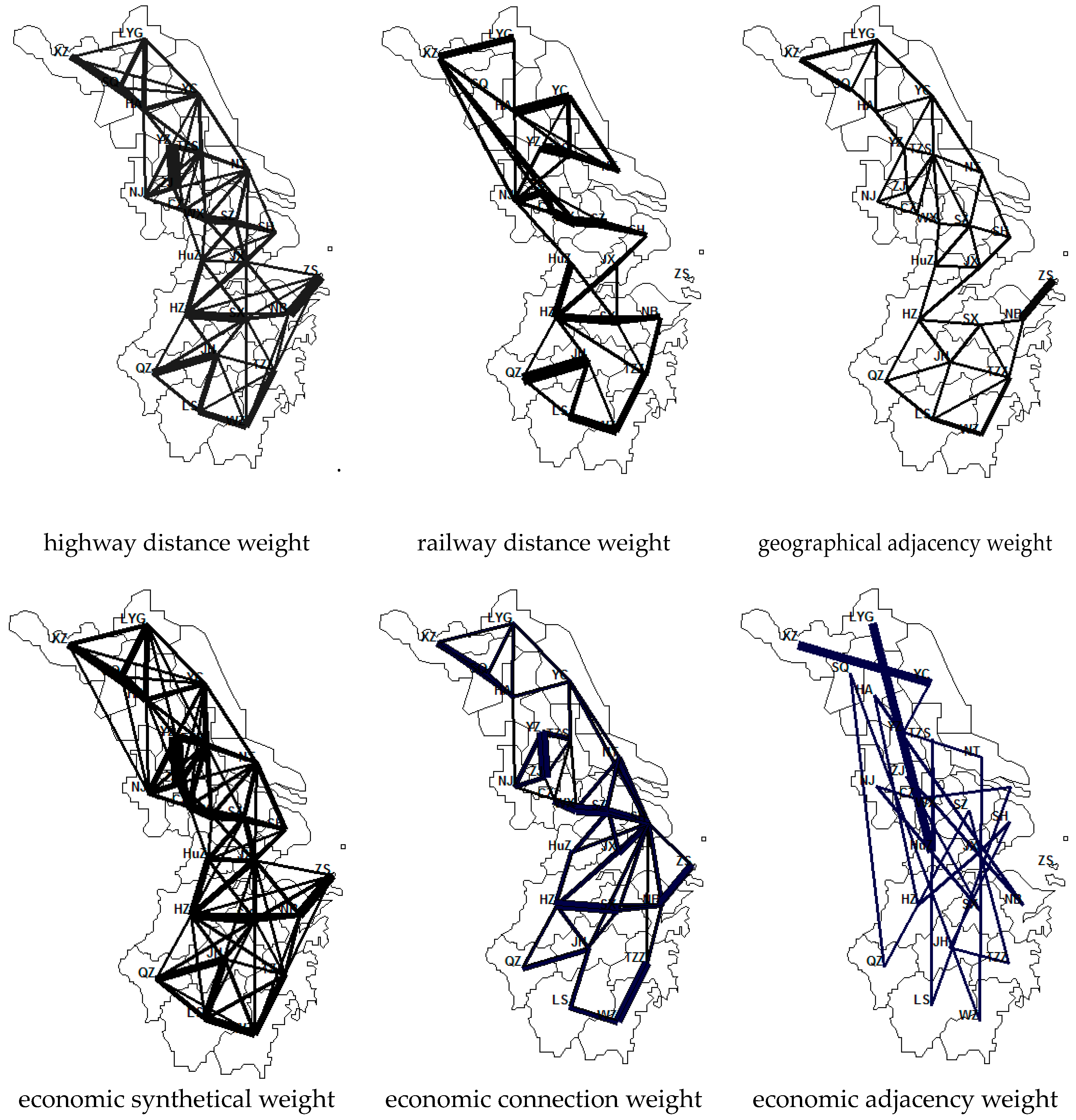
We set six different weight matrices, namely, the geographic distance (of highway and railway) weight matrix, the geographical adjacency matrix, the economic distance (of GDP and economic linkage) matrices, and the economic adjacency matrix, to depict the housing spatial correlation in the Yangtze River Delta Urban Agglomeration. Among these matrices, the highway distance weight matrix takes the reciprocal square of the highway distance between cities as element, the railway distance weight matrix takes the reciprocal square of the railway distance between cities as element, the geographical adjacency weight matrix takes the element of one when cities are adjacent to each other and zero when cities are not adjacent under the Queen rule, the economic distance weight matrix takes the GDP difference quotient and the geographical distance between cities as element, the economic connection weight matrix takes the economic linkage degree between cities as element which is calculated by R
ij as previously, and the economic adjacency weight matrix takes the element of one when cities are closest to each other in per capita GDP and zero when they are not. The results of the six weight matrices are illustrated in
Figure 1, wherein the thickness of lines represents the degree of spatial link between cities.
5. Spatial Correlation Test Results with Moran’s I method
Moran’s I index of spatial autocorrelation is widely used to observe the correlation between spatial variables [
22] while the local Moran’s I, LISA index, and Moran’s I scatter plot are commonly used to describe spatial correlations among regions. When the LISA test is significant, a positive correlation implies that a spatial agglomeration exists in the region, including high-high and low-low cases, whereas a negative correlation implies a spatial outlier, which includes high–low and low-high cases [
44].
First, Moran’s I indices of the prices of newly built houses in the 25 cities of the Yangtze River Delta from 2000 to 2013 were calculated. The results presented in the second and third columns of
Table 2 are based on the Queen adjacency weight matrix, while the fourth and fifth columns are based on the K-nearest (K takes six in this case, as usual) weight matrix. Queen adjacency refers to regions with a common boundary or node, and K-nearest denotes the k neighbor cities closest to a certain place.
Table 2 shows that the Moran’s I value in the second and fourth columns are close to each other, and that the results are all significant at the 5% level after 2005, which indicates a significant positive correlation between the 25 cities in the Yangtze River Delta.
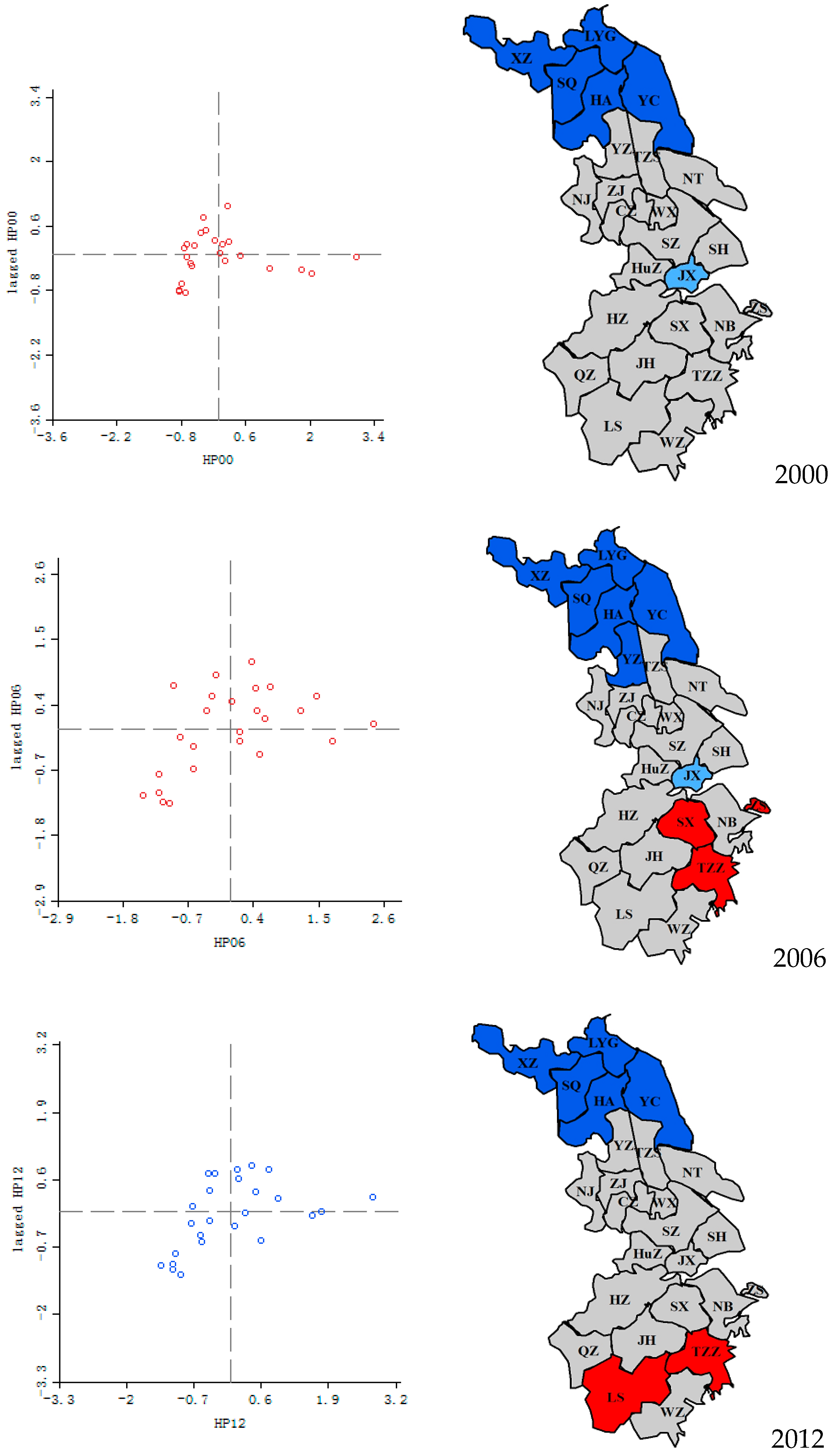
We then drew the Moran’s I scatter plot and LISA cluster map of a certain year. The top line of
Figure 2 shows the local agglomeration in 2000, in which Zhoushan, TaizhouZ (which stands for Taizhou city in Zhejiang province), Changzhou, and Suzhou are located in the first quadrant, forming a high–high cluster with a positive spatial correlation; Jiaxing, Huzhou, Shaoxing, Nantong, Quzhou, Jinhua, and Zhenjiang are in the second quadrant, constituting a low–high cluster with a negative spatial correlation; Lishui, Yangzhou, TaizhouS (which stands for Taizhou city in Jiangsu province), Yancheng, Suqian, Xuzhou, Huaian, and Lianyungang are in the third quadrant, comprising a low–low cluster with a positive spatial correlation; and Shanghai, Ningbo, Wenzhou, Nanjing, Wuxi, and Hangzhou are in the fourth quadrant, forming a high–low cluster with a negative spatial correlation. Generally, the number of cities in Quadrants I and III is approximately equal to that in Quadrants II and IV, which means that spatial autocorrelation is not evident in 2000. The LISA map shows that the cold-spot cluster (where house prices of both the city and adjacent cities are low) consists of five cities in the northern region of Jiangsu province.
The middle line shows the Moran’s I scatter plot and the LISA cluster map for 2006. Compared with the results for 2000, more cities are located in Quadrants I and III. Shanghai, Suzhou, Ningbo, Zhoushan, Jinhua, Lishui, Wenzhou, TaizhouZ, and Shaoxing are in Quadrant I; eight cities in Jiangsu are in Quadrant III, which shows a strong spatial autocorrelation. In addition, the cold-spot cluster is concentrated in the northern region of Jiangsu, whereas the hot spots (where house prices in both the city and adjacent cities are high) appeared in Zhoushan, Shaoxing, and Taizhou in Zhejiang.
The Moran’s I scatter plots indicate the same distribution since 2006. The last line in
Figure 2 shows that 16 cities are located in Quadrants I and III in 2012, accompanied by strong spatial autocorrelation. In the LISA map, the cold spot is still grouped in North Jiangsu, and Jiaxing in North Zhejiang still as an outlier in the region, while Lishui and TaizhouZ in South Zhejiang as the new hot spots,
Based on the Moran’s I scatter plot and the LISA plots of three cross sections, we were able to find steady connections between house prices with the housing market development. The cold spot was always located in North Jiangsu, which indicates a stable local spatial correlation. By contrast, the hot spot in Zhejiang experienced a moving mode of “Jump,” indicating that the connection between markets may depend on information interaction or some other factors, rather than commuting or migration.
6. Results from the Spatial Panel Model
By adopting the spatial panel data model, weight matrix, and variables discussed in the previous section, this section estimates the spatial spillover effect of housing prices in the Yangtze River Delta and compares the results derived from different models and weight matrices.
6.1. Model Comparison
First, given that the research object comprised all the 25 prefecture-level cities in the Yangtze River Delta urban agglomeration, that is, the individuals in the observed sample were not randomly selected from a large sample, the fixed effect was a better choice compared to random effect [
45]. The LR test for spatial-/time-fixed effect further indicated that the spatial fixed effect was appropriate according to the better R
2 and corr
2 statistics for the panel data models. Subsequently, the SAR, SEM, and SDM were estimated in the highway distance weight matrix and corresponding tests were carried out; the results are shown in
Table 3. By comparing the regression results in functional forms of linear, logarithmic, and log-linear, we found that both the goodness of fit and significance of the variables were the best in logarithmic form. All the variables were taken in log form except for the two ratio indices, i.e.,
industry, green. The LM (Lagrange multiplier) and Robust LM tests rejected the null hypothesis at the 5% significance level which meant that the spatial model should be adopted in this study instead of the non-spatial model. Moreover, the Wald and LR tests rejected the null hypothesis of simplifying the SDM into SAR or SEM. Thus, it was determined that SDM should be employed in this study, which was in line with theoretical expectations.
6.2. Regression Results in Different Matrices
The six matrices revealed different spatial relations between cities. This section estimates the spatial panel model under those different matrices, and the results are shown in
Table 4.
By observing the regression results of all variables in a certain matrix (the highway distance weight for instance), we were able to see that the coefficient value of the spatial lag is 0.65, which means that the spatial lag has a significant positive impact on house price; the coefficient of pop is 0.12, which means that a 1% change in the population variable will result in a 0.12% synchronous change in house price; and the coefficients of the W × industry and the W × green are 0.61 and 0.57, respectively, which means that the industry structure and green level in neighboring cities will substantially affect local house prices.
The regression results in different matrices were then compared. The spatial lag coefficients were always significant under different matrices, showing that spatial lag generally has a stable influence on the performance of house prices. However, the value in the economic matrix was greater than that in the geographic matrix, which means that economic linkage is more important for the housing spillover than geographical linkage. The same condition holds for the W × industry, whose coefficient was greater in the economic matrix than that in the geographic matrix, indicating that industry spillover strongly influences house prices in cities with tight economic association. In addition, the coefficients of W × green were significant in all six matrices, which shows that the natural environment of the entire urban agglomeration positively influences urban house price. In summary, the results for each matrix were similar, but the R2 in the railway distance and economic adjacency weights were relatively lower than those in other matrices.
6.3. Direct and Indirect Effects
The spatial panel model outperforms regular panel data models because it can distinguish the direct and indirect effects of independent variables. The direct effect measures the degree of influence on local house prices when the independent variable changes a unit, whereas the indirect effect measures the degree of influence on neighboring house prices when the independent variable changes a unit.
Table 5 presents the direct and indirect effects of all variables on house prices in all six matrices.
The results show that disposable income has a more significant indirect effect, which means that income growth will increase house prices in neighboring cities more than in local cities. The same result holds true for the proportion of the tertiary industry. Population size has a significant direct effect on house prices within the local market but is not significant for the indirect effect and a negative indirect effect with economic adjacency weight, which means that population growth will exert a backwash effect, that is, the negative influence of the core city’s growth on the periphery. Green coverage has both significant direct and indirect effects which means that green levels will affect house prices throughout the entire region, i.e., in both local and neighboring cities.
6.4. Findings
Based on the regression results, we can draw the following conclusions.
First,
the overall economic development and natural environment have a common impact on house prices in each city. Based on the indirect effect, disposable income, the proportion of tertiary industry, and green coverage have significant spillover, indicating that an increase in income and a high proportion of the tertiary industry in a local city will increase house prices in other cities. In addition, overall environmental livability significantly explains house prices in the Yangtze River Delta. Thus, house prices in the region are positively affected by the overall economy and natural environment, which conforms to the investment distribution in the Yangtze River Delta laid by major property companies in practice. Government policies are important factors determining house prices and household location selection between the central city and suburbs [
46]. Policies such as improving the natural environment, adjusting economic structure, and increasing the ratio of the tertiary industry are generally implemented in the urban agglomeration of Yangtze River Delta and are conducive to improving the housing market in all cities.
Second, cities with similar economic levels compete in real estate markets. With regard to the results of the economic adjacency weight matrix, the coefficients of W × pop and W × techq were negative, which implies that cities with economic adjacency have population and talent competition which will eventually result in a negative correlation in house prices. By contrast, this phenomenon is absent in most of the other weight matrices. Therefore, real estate markets of cities with economic proximity appear to compete for population. In addition, due to the role of the government, population growth restriction policies in large cities and talent attraction strategies in each city make the population concentrated in central cities and dispersed within other cities. Furthermore, competition for human capital has for this reason formed among cities.
Third, geographical and economic distances have similar influences on house prices in cities. Models with geographical and economic distance weight matrices showed similar regression results. The spatial lag of house prices was always significant at the 1% level. By contrast, the coefficients of W × hp in the two adjacency matrices achieved minimum values of 0.48 and 0.35, which means that the spatial spillover effect of house prices in the Yangtze River Delta is not confined to a geographically or economically adjacent city. The comprehensive linkages in geography and economy play a significant role in the spatial diffusion of house prices. Furthermore, the coefficient in the geographical distance matrix was slightly smaller than that in the economic distance matrix. Thus, economic connection plays a more significant role in causing spatial spillover than the geographical tie. However, the difference is not too large because the economic connection is still based on geographical proximity to some extent.
Lastly, city status, urbanization level, and the ability to transform and upgrade positively influence the spatial relations of house prices. By grouping the 25 cities according to their economic linkage with the center city, urbanization level, industrial structure, and innovation ability, cities with high characteristic values were grouped together, whereas cities with low characteristic values were grouped in another set. The city group was estimated with different features to observe the spatial spillover performance of house prices in the Yangtze River Delta. The results based on highway distance weight are shown in
Table 6.
The first group is divided by their economic linkage with the central city. The 12 cities closely linked to the central city have a larger spatial lag coefficient (0.65) than the other 13 cities (0.28), which means that the spatial correlation is stronger among cities with closer linkages to the central city.
The second group, which is divided by urbanization level, shows that cities with a high urbanization level have a larger spatial lag coefficient and a stronger spatial correlation than other cities. This result could be explained by the development mode mentioned in
Section 3. A city in the early stages of urbanization expands its scale mainly through population growth and capital investment, whereas a city in advanced stages relies more on technology and innovation to develop itself. Considering that technology has more flexible communicability and stronger coupling effect than manpower and capital, cities with higher urbanization levels achieve stronger spatial spillover in economic fields such as the housing market.
The third group is divided by industrial structure. With the upsurge in regional integration and the differentiation of positioning, the industrial layout of cities in the Yangtze River Delta differs gradually. Generally, cities with strong economic power experience industrial transformation and upgrade. Thus, interactive economic activity and frequent exchanges in personnel, capital, and information cause a stronger spatial effect on house price in cities with a higher tertiary industry proportion, as confirmed by the results in the third row of
Table 6.
Similarly, the last group is divided by innovation ability. With patent grants by proxy, house prices in cities with high innovation abilities also exhibit a strong spatial correlation.
Generally, the difference in the position of inner urban agglomerations and urbanization levels will result in a corresponding disparity in the spatial correlation in house prices. Specifically, cities with close economic linkages with the center city, high urbanization levels, optimized industrial structures, and strong innovation abilities have high levels of spatial spillover effect. The results verify our assumption that a strong house price correlation exists among cities with similar characteristics in a city group, which has not been mentioned in previous studies.
7. Conclusions
This paper presents an empirical study on the spatial spillover effect of house prices in 25 cities in the Yangtze River Delta in China based on annual panel data for the period 2000 to 2013. By constructing a non-spatial model, it can be observed that market demand and livable environment factors, namely, per capita disposable income, tertiary industry proportion, urban green spaces, population size, and house sales volume, significantly influence house prices in the Yangtze River Delta. However, the Moran’s I and LISA tests indicate that the spatial correlation of house prices exists throughout the study period, especially after 2005.
When considering spatial correlation, the income variable does not display an evident effect on house price; the spatial lag of house prices instead plays a dominant role, and the Yangtze River Delta has a significant spillover effect on house prices. Furthermore, the proportion of the tertiary industry and urban greening have a significant indirect effect on the house prices of neighboring cities, and this condition is more evident in the economic distance weight matrix than in the geographical distance weight matrix. Finally, there are different degrees of spatial dependence of house prices in the region, and cities with close economic linkages with the center city, high urbanization levels, optimized industrial structures, and strong innovation abilities, show high levels of spatial spillover effects.
The Yangtze River Delta urban agglomeration has formed a multi-center spatial network structure. The overall economic development and urbanization processes have reached the post-industrialization stage and moved toward the developed economy period. Developed transportation networks and close industrial interactions between cities have established strong correlations in regional house prices. The spatial spillover effect detected in the area confirms that the coordinated development of the natural environment and economic development among the cities promotes the spread of housing prices, while population mobility, especially the competition of technical talents, cause a backwash effect. Differences were observed in the spillover effect of house prices among urban groups divided by industrial structure and innovation ability. This finding reveals the impact of economic transition on the real estate market. However, the difference in the spatial correlation of house prices between cities should also be considered, especially the differentiation trend caused by linkages with the center city. Both real estate investors and government administrative departments should consider these conditions carefully to avoid investment risk and to effectively improve policy outcomes.


