Abstract
With the rapid development of grid-connected wind power, analysing and describing the probability density distribution characteristics of wind power fluctuation has always been a hot and difficult problem in the wind power field. In traditional methods, a single distribution function model is used to fit the probability density distribution of wind power output fluctuation; however, the results are unsatisfying. Therefore, a new distribution function model is proposed in this work for fitting the probability density distribution to replace a single distribution function model. In form, the new model includes only four parameters which make it easier to implement. Four statistical index models are used to evaluate the distribution function fits with the measured probability data. Simulations are designed to compare the new model with the Gaussian mixture model, and results illustrate the effectiveness and advantages of the newly developed model in fitting the wind power fluctuation probability density distribution. Besides, the fireworks algorithm is adopted for determining the optimal parameters in the distribution function model. The comparison experiments of the fireworks algorithm with the particle swarm optimization (PSO) algorithm and the genetic algorithm (GA) are carried out, which shows that the fireworks algorithm has faster convergence speed and higher accuracy than the two common intelligent algorithms, so it is useful for optimizing parameters in power systems.
1. Introduction
Owning to the increased efficiency of clean energy, and the need to reduce pollution and fuel consumption, development in renewable energy sources, including wind power plants, is of great significance [1]. With wind generation technologies improving, this form of energy production becomes a valuable alternative to conventional energy sources [2]. The proportion of energy generated by wind is increasing due to recent technology and efficiency improvements, as well as government funding [3]. A challenge in using wind power is the uncertainty in the wind resource. [4]. The output of wind power is limited by the wind speed, which is different from a conventional synchronous generator, and the unit output has strong random, undulating and intermittent characteristics [5]. Therefore, large-scale wind power access system brings severe challenges to the safe and stable operation of the power grid.
In wind power systems, large disturbances such as short circuit faults often occur in addition to small wind power disturbances during regular wind speed operation. These disturbances increase wind power randomicity, thus leading to instability of the power systems when wind power is connected to electricity grid. As the wind power capacity of the grid increases, more and more attention has been paid to the possible impact caused by wind power randomicity [6]. Random wind power fluctuation is considered the main factor which affects the quality of power systems; therefore, the wind power fluctuation characteristics are the basis for further research. The analysis of the wind power output characteristics is another way to cope with the uncertainty of wind power effectively [7,8]. Moreover, the wind power fluctuation impact on the power grid can be more clearly demonstrated by analyzing the fluctuation characteristics. In fact, the wind power fluctuation characteristics could also be used in wind farm planning as a forecasting technique, because the output duration curve could be forecast from studying wind power fluctuation. The reason for the inaccurate forecasting of wind power is that we still cannot accurately grasp the fluctuation characteristics of wind power. So, research on the fluctuation characteristics of wind power has an important significance not only for overcoming the harmful effect caused by wind power connected to the electricity grid, but also for improving the prediction accuracy of wind power.
Currently there are mainly two ways of describing wind power randomicity. One is on the basis of stochastic sequences, and the other is on the basis of probability density function. In recent years the probability density function methods based on statistical theory have become very widespread in investigating the wind power fluctuation characteristics and its quantitative analysis [9,10,11,12]. The influence of wind power fluctuation on stability of power systems has attracted more and more attention along with increasing scale of the wind power integration. Therefore, describing the probability density distribution characteristics of wind power fluctuation has always been a challenge in grid-connected wind power operation analysis. The central idea is that the probability distribution of wind power fluctuation is fitted by a theoretical distribution function curve, realizing that the wind power change law is described by the existing distribution function model. Lin et al. [13] adopted the minute-scale as an index for depicting the wind power fluctuation and discovered that the location-scale distribution can serve to describe the wind power fluctuation law of minute scale component. They had also come to similar conclusions based on power data of the European wind farms [14]. Zhang et al. [15] and Yang et al. [16] described the change law of wind power prediction error using the normal distribution and optimized beta distribution model, and the wind power fluctuation range was estimated from the distribution function characteristics. Xia and his collaborators [17] analyzed the probability distribution law of short-term power sags in wind power, and employed the generalized Pareto distribution for modeling the probability distribution characteristics. Zhang et al. [18] divided the probability density distribution of wind power prediction error by interval, and proposed a multi-objective optimal economic dispatch model. Zhou and Liu et al. [19,20] used normal distribution function model for modeling the wind power time series output with different methods.
In the above studies, the authors chosen the probability density distribution function with the optimal fits. However, fitting effects are also restricted by the subjective classification of the indicators and the type of the chosen distribution functions. Meanwhile, some studies have demonstrated that the wind power fluctuation varies with different space and time, and the global optimal probability density distribution function of the same fluctuation indicator is not always the same [16,21,22]. Fan et al. [23] utilized the normal distribution to express the wind power prediction error distribution, but the distribution curve of the distribution function model is much more different from that of the prediction error. Vladislovas and his collaborators [24] investigated wind power density distribution at location with low and high wind speeds using the Weibull model and provided four numerical methods for evaluating Weibull parameters. Pishgar-Komleh and others [25] applied Weibull and Rayleigh distribution functions to find out the best fitting tool in order to determine the wind power density and the available energy. However, it can be observed from the results that at some wind speeds there are significant errors between the models and the observed data.
The above studies exhibit the problems associated with wind power fluctuation characteristics based upon probability density function analysis. The distribution function model may fit several distributions which occur in the actual wind farm poorly, so only the distribution function models with relatively fine fitting effect can be chosen to characterize the wind power fluctuation. Other work [26] indicates that the overall wind power fluctuation distribution cannot be satisfied with a single specific distribution function model when analyzing the wind speed and wind power scatter plot of the actual wind farm. However, there is no in-depth study on reasons for this and improvement measures. Over the past years, a Gaussian mixture model has been applied in grid-connected wind power operation analysis owning to its flexibility [27,28,29]. Cui et al. [27] presented a Gaussian mixture model to fit probability density distribution instead of a single distribution function model; the model works well and is applicable to large-scale wind farms. Likewise, Ge et al. [28] used the Gaussian mixture model for the wind power forecast error model, and the suitability of the model was verified. Liu et al. [29] proposed a probabilistic modeling method based on the expectation constraint maximization algorithm to improve the simulation accuracy of the weighted Gaussian mixture model.
However, the Gaussian mixture model has more parameters, making implementation more complicated and increasing the amount of computation.
Addressing the shortcomings in previous work, a new distribution function model with four parameters is established in this paper in order to better fit the probability density distribution of wind power fluctuation. The parameters in the model are captured through the fireworks algorithm. The model validity is verified based on six simulation experiments and the fireworks algorithm superiority is demonstrated through comparison experiments.
This study provides a modeling method for the probability distribution of wind farm group output power fluctuation, which makes up for the deficiency of a quantitative method for describing the wind power fluctuation, thus is an important supplement in this field. The proposed model also provides an analytical tool and prediction technology for wind farm construction planning. Besides, the work offers a more rapid and effective optimization method for finding model parameters.
2. Problem Statement and the New Distribution Model
As an example case, the measured data from a wind farm group is considered and its wind power fluctuation probability distribution is analyzed. The wind farm group includes 7 wind farms, and its capacity is 450 MW. Figure 1 provides the wind power probability density distribution at 5 min/ point sampling interval of the wind farm group.
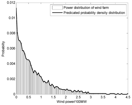
Figure 1.
Probability density distribution of the wind power fluctuation.
It is observed from Figure 1 that the probability density distribution curve shows a downward trend as a whole, but it is not monotonically decreasing. The probability density distribution characteristics of wind power fluctuation are of “trailing” property. Owning to the “trailing” distribution characteristics, some researchers have chosen single distribution functions such as normal distribution, location-scale distribution, generalized extreme value distribution and Weibull distribution for the purpose of fitting wind power probability density distribution [12,13,14,15,16,17,18,19,24,25].
However, the experimental results in the literatures have validated that (1) the single distribution function has a poor effect in fitting the probability density distribution of wind power fluctuation; (2) the variation law of wind power fluctuation is not consistent with a single distribution function; (3) when the “fluctuation smoothing effect” of the wind farm group cannot completely eliminate the fluctuation characteristics of a wind farm power output, the output fluctuation characteristics of the wind farm group will not satisfy a specific distribution function.
Therefore, in the literatures [27,28,29] the Gaussian mixture model is presented for fitting wind power fluctuation probability density distribution instead of those single distribution function models. The mathematical expression of the Gaussian mixture model is:
where , and are distribution parameters of the Gaussian mixture model.
Later in Section 4, statistical indexes are used to make a quantitative comparison of how well different distribution function models fit the data. Compared with a single distribution function, the fitting effect of the Gaussian mixture model is obviously much better, and the advantages are more prominent. But the model is at least the second-order, so no less than 6 parameters need to be solved. For the fifth-order model, 15 parameters need to be solved, resulting in much more computation.
In this paper, a new distribution function model is proposed to fit the measured power probability distribution data of wind farm groups, and the model includes only four parameters, which will greatly reduce the complexity and computation.
2.1. A New Distribution Model
As analysed previously, the measured data indicates that wind power fluctuation probability density distribution takes on an overall declining trend, and has “trailing” property. Therefore, consider the following function that defines the domain [30,31]:
where, ,,. , , and are constants, and are for regulating the position of in the range of , while is for regulating the amplitude of .
Obviously , and holds, that is,
From (3) we can know that is the normalization coefficient, and rearranging this:
The derivative of is:
Let
then Equation (5) is rewritten as:
The roots of the equation represents the extremum positions of , and their properties will affect the shape of .
2.2. The Shape of the Function
As , the equation is a third-order algebraic equation. The shape of the function is closely related to the properties of roots of and the function value at .
For example, when , , this indicates that only make pass through the origin, otherwise .
If , Function (2) is turned into the following:
Let the derivative of in (8) be equal to zero,
then the roots of the above equation are:
So, the shape of is single-peak passing through the origin.
After analyzing the other cases in the same way, there are five shapes possible for [26] as shown in Figure 2 and described below:
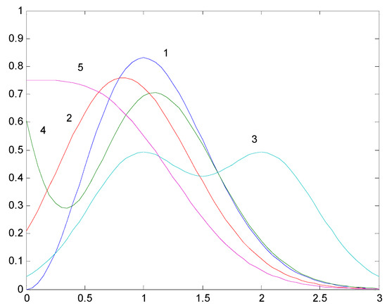
Figure 2.
Shapes of .
(i) When , is of single-peak shape and passes through the origin (curve 1 in Figure 2);
(ii) When has one positive real root, is of single-peak shape without passing through the origin (curve 2 in Figure 2);
(iii) When has three unequal positive real roots, is of double-peak shape without passing through the origin (curve 3 in Figure 2);
(iv) When has three distinct real roots, and the two are positive, is of one and a half peak shape (curve 4 in Figure 2);
(v) When has no positive roots, or has two equal positive real roots and the third root is no more than zero, is of non-peak shape (curve 5 in Figure 2).
From the above analysis we can see that there are several shapes for the function including non-peak, single-peak, double-peak and so on, naturally including the probability distribution with the “trailing” property, thus the function can be adopted to describe the wind power fluctuation probability density distribution.
3. Fireworks Algorithm
3.1. Introduction to Fireworks Algorithm
The fireworks algorithm is a novel swarm intelligence algorithm with an explosion searching mechanism, that can be used to search for global optimal solution. The fireworks algorithm shows very excellent performance and high computational efficiency, and thus, has gradually become a proven swarm intelligence algorithm [32,33].
When a firework is set off, the local space around the firework will be filled with a shower of sparks. Figure 3 provides two common cases for a firework explosion, and fireworks with different quality will produce different effects when they explode. Good fireworks produce more sparks, and the range of sparks produced in the explosion is also relatively concentrated. On the contrary, poor fireworks produce fewer sparks, and the range is relatively dispersed. In this way the fireworks algorithm establishes a mathematical model by simulating the exploding behavior of fireworks in the air. The algorithm has formed an explosive search method by introducing random factors and selection strategy, and thus developed into a global probability searching method which can work out the optimal solution for complicated optimization problems. Therefore, the explosion process of a firework can be regarded as a search in the local space around a specific point [32].
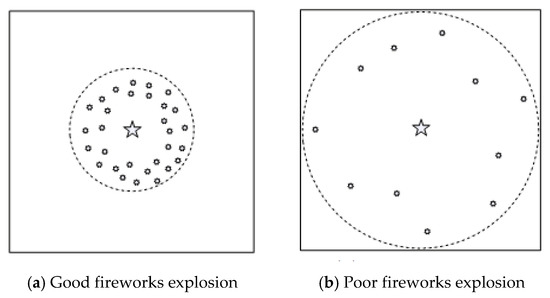
Figure 3.
Two kinds of fireworks explosion.
Without loss of generalization, the optimization problem to be solved usually can be transformed into the following minimization optimization problem:
where, is the objective function, and is the feasible region of solutions. The ultimate objective of working out the optimization problem (11) using the fireworks algorithm is searching for a point in , and making obtain a minimal fitness value at a global scope.
In our work, we take the performance index function as the fitness function, so our goal is to get the optimal value of the model parameters so that the performance index function value is the smallest, that is, the fitness value is the smallest. Therefore, the fireworks with better fitness value in the fireworks algorithm refer to the fireworks with smaller fitness value, i.e., the parameters obtained with smaller fitness value. When these fireworks explode, the more sparks and the smaller explosion amplitude are produced. More sparks can avoid the sparks always swing near the optimal value, and cannot find the optimal value accurately. Smaller explosion amplitude can converge to each extremum more effectively and find the optimal solution ultimately. So, this principle is based on the type of problems to be solved and the fitness function design method. To sum up, for the fireworks with small fitness function value, more sparks and smaller explosion amplitude are generated; for the fireworks with larger fitness function value, the fewer sparks and the larger explosion amplitude are generated.
Generally, the fireworks algorithm consists of explosion operator, mutation operation, mapping rules and selection strategy. The explosion operator mainly includes explosion intensity, explosion amplitude and displacement operation. Mutation operation is primarily Gaussian mutation operation. Mapping rules mostly include modulo operation rules, specular reflection rules and random mapping rules. Selection strategies primarily contain selection distance and random selection. The framework of the fireworks algorithm is shown in Figure 4.
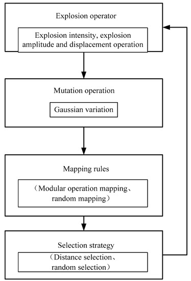
Figure 4.
The framework of the fireworks algorithm.
3.2. Algorithm Flow
The fireworks algorithm starts iteration and makes use of explosion factor, mutation factor, mapping rule and selection strategy in turn until the termination condition is reached, i.e., the precision requirement of the problem is satisfied or the maximum times of function valuation is achieved. The fireworks algorithm includes the following steps:
(1) Some fireworks are generated randomly in a given solution space, and each firework represents a solution in the solution space.
(2) Calculate the fitness value of each firework according to the fitness function and generate sparks according to the fitness value. The better the fitness value is, the more sparks are produced.
(3) Sparks are generated in the radiation space of the fireworks (the explosion amplitude of a firework is determined by the fitness function value, the smaller the fitness value, the smaller the explosion amplitude, and vice versa). Then each spark represents a solution in the solution space. In order to ensure population diversity, it is necessary to make appropriate variation for the fireworks, such as Gaussian mutation.
(4) Calculate the optimal solution of the population and determine whether or not it satisfies the requirement. If satisfied, stop searching, otherwise continue iterating. The initial values of the iteration are the solutions obtained from this cycle.
The basic flow of the fireworks algorithm is shown in Figure 5.
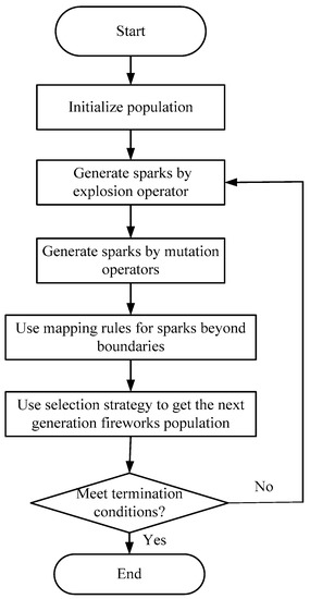
Figure 5.
The basic flow of the fireworks algorithm.
4. Statistical Index Models to Analyze Distribution Function Fits
When the probability density function method is used to study the wind power fluctuation characteristics, a theoretical distribution function is chosen for describing wind power fluctuation. The fitting effect of the distribution function can be quantified by means of residual sum of squares (RSS), root mean square error (RMSE), determination coefficient and adjusted determination coefficient, etc. RSS and RMSE are used to calculate the fitting error value between the distribution function model and wind power fluctuation probability density distribution, reflecting the fitting effect from the error aspect. Determination coefficient and adjusted determination coefficient can be used to characterize the effectiveness of the distribution function model fit through changing data sets.
(1) Residual Sum of Squares (RSS)
RSS represents the squared sum of the errors between sample data of each array and the mean of the data, reflecting the discrete case of each sample. Define the variable to express the RSS index value.
where, is the corresponding function value of the distribution model at one level, is the wind power probability at the same level, is the installed capacity. Simply speaking, the smaller the RSS of a set of data, the better the fitting effect of the distribution function model.
(2) Root Mean Square Error (RMSE)
RMSE represents the error between the estimated values of the model and the original values. The closer to 0 the RMSE value, the better the fitting effect of the model. Define the variable to express RMSE index value, whose computational formula is:
(3) Determination Coefficient
Determination coefficient is a statistic which makes comparison among models, and directly judge whether the fitting is good or bad. Define to represent the determination coefficient, whose computational formula is:
where, represents a square sum of the difference between the original data and the distribution model data, represents a square sum of the difference between the original data and the mean . The range of is [0,1], the closer to 1, the stronger the model’s ability to explain the samples, the better the model fits with the data.
(4) Adjusted Determination Coefficient
Adjusted determination coefficient is used to evaluate merits and drawbacks of the distribution model. But as the number of independent variables increases, will continue to increase. Therefore, in order to achieve comparative fairness, it is necessary to consider the influence of the number of distribution parameters when comparing the fitting effect of the distribution function models with different number of distribution parameters. Define the variable to express the index value of the adjusted determination coefficient.
where, is the dimension of data, and is the number of the parameters in the model. The range of is [0,1], the closer to 1, the better.
In this work, the above four evaluation indexes will be used to make a quantitative comparison for the fitting effects among different distribution function models.
5. Numerical Simulation Verification and Validation
This section outlines our simulation verification and validation process. Using measured data, we calculated the probability level for fluctuations in the wind power output. Then, we used the proposed new distribution model for fitting the probability density distribution of wind power fluctuation.
First, we select the performance index function for the studied problem as follows:
and take the new distribution function model to replace ,
where, refers to the wind power value.
Our goal is to use the proposed distribution model to fit the wind power probability density distribution by finding optimal parameters , , and to make minimum. These parameters are optimized through the fireworks algorithm. Using the fireworks algorithm, the parameters are viewed as the fireworks in the algorithm. The number of parameters is the same as the dimension of each firework. The performance index function is taken as the fitness function in the fireworks algorithm, and the sparks after the fireworks explodes can be used as the next generation fireworks. Evaluate their fitness values, if the current fireworks make the fitness value the minimum, then it stops exploding. The fireworks at this time are the optimal solution to the studied problem, that is, the best parameter values. Then, the model is closest to the wind power probability density distribution.
In the simulations we measured the output power of seven wind farms (W1, W2, …, W7) for every 5 min interval. The research objective is be able to analyze single wind farms to large-scale wind farm groups, so in this work the probability density distribution research will gradually converge from a single wind farm with small capacity to large-scale wind farm group. The convergence principle is to gradually converge the wind farms in the order of their installed capacity from small to large [34].
To verify the proposed distribution model (NDM), we compare it with the second-order Gaussian mixture model (SGDM) and the fifth-order Gaussian mixture model (FGDM) by fitting the wind power fluctuation probability density function for each to the wind farm fluctuation data distribution (PFDD).
In the simulation results for each optimized solution using these methods is shown for the wind farm configurations in Figure 6a–f, which represent the fitting with the wind power fluctuation probability density distribution for the wind farm groups. W1–W2 means the convergence of wind farms W1 and W2, W1–W3 means the convergence of wind farms W1, W2 and W3, and so on.
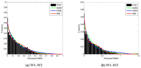
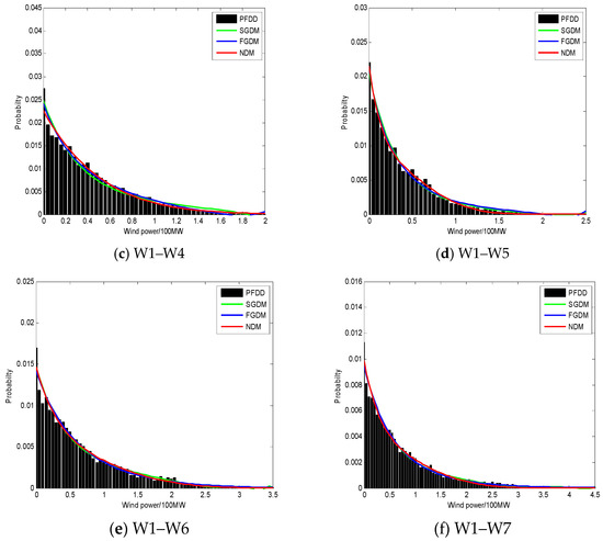
Figure 6.
Fitting with the wind power fluctuation probability density distribution for different wind farm groups.
Meanwhile, four statistical index values (, , and ) of the three models are listed in Table 1, Table 2, Table 3, Table 4, Table 5 and Table 6, and the run times (/s) of three models are also recorded when conducting simulation experiments.

Table 1.
Statistical index values and run time for fitting W1–W2.
Table 2.
Statistical index values and run time for fitting W1–W3.
Table 3.
Statistical index values and run time for fitting W1–W4.
Table 4.
Statistical index values and run time for fitting W1–W5.
Table 5.
Statistical index values and run time for fitting W1–W6.
Table 6.
Statistical index values and run time for fitting W1–W7.
Table 7 offers the parameter values of the proposed wind power probability distribution model.
Table 7.
Parameter values of the NDM.
In order to prove the superiority of the fireworks in the convergence speed and error accuracy, our optimization methodology was compared with the particle swarm optimization (PSO) method and the genetic algorithm (GA) method by doing additional simulations, and the data used is from the convergence of wind farms W1-W7. The convergence rate can be measured by the number of iterations, and error precision is defined as the same form as the performance index function ().
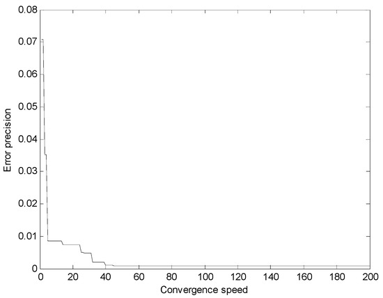
Figure 7.
Convergence speed and error precision of the PSO algorithm.
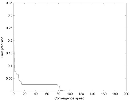
Figure 8.
Convergence speed and error precision of the GA.
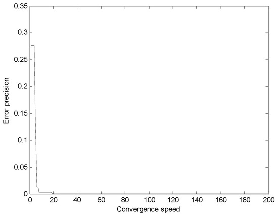
Figure 9.
Convergence speed and error precision of the fireworks algorithm.
The convergence speed and error precision for three intelligent algorithms are listed in Table 8.
Table 8.
Convergence speed and error precision of three intelligent algorithms
6. Results Discussion
Observing Figure 6a–f in the simulation results, three distribution models can all fit the wind power fluctuation probability density distribution. However, it is obvious that our new model has the best fits with the actual data distribution among the three models. On the whole, the fifth-order Gaussian distribution model is relatively better than the second-order Gaussian distribution model in goodness of fit. At the same time, we noticed that when fitting the convergence for wind farms W1–W7, goodness of fit for the second-order Gaussian distribution model is almost the same as the fifth-order Gaussian distribution mode, which illustrates that potentially only the second-order Gaussian mixture distribution model is needed to fit the data.
Moreover, it is seen from Table 1, Table 2, Table 3, Table 4, Table 5 and Table 6 that and of the new distribution function model are the smallest of the three cases, and and of the new distribution model are closest to 1. In fact, if and are fixed, according to the formula , the adjusted determination coefficient increases as the number of the model parameters decreases. Therefore, the fewer parameters the model has, the closer approaches 1. The parameters of the new model are the fewest, so it is most beneficial for calculating .
Furthermore, it is worth highlighting from Table 1, Table 2, Table 3, Table 4, Table 5 and Table 6 that in six wind power groups, the run time of our new model is much shorter than that of the two others, and that is because the number of the parameters in the new distribution model is the lowest of three models, which makes the calculation much easier, indicating the superiority of the new distribution model.
In addition, we can also see from Figure 6a–f that with the gradual expansion of the wind farm group, the probability of zero output is gradually reduced. This is because when the output of one wind farm is zero, the output of another wind farm is possibly not zero due to the intermittentity and randomness of wind energy. Consequently, they can compensate for each other.
Finally, from the comparison results in Figure 7, Figure 8 and Figure 9 and Table 8, it can be seen that the convergence speed of the fireworks algorithm is the fastest among the three intelligent algorithms. For the fireworks algorithm only about 20 iterations are needed to achieve the stable error precision, followed by the PSO algorithm, which needs 44 iterations, and then the GA, which needs 91 iterations to converge. The convergence speed of the fireworks algorithm was obviously outstanding, and the success lies in a good design of the explosion process and a proper method for selecting locations. The search mechanism of the fireworks algorithm is efficient, while the GA needs to select, copy and mutate operations, so the number of iterations is the largest. From Table 1 we also notice that the error precision of the fireworks algorithm is the smallest, and the error level reaches 10−6. Although the GA has more iterations, its error precision is smaller than that of the PSO algorithm.
7. Conclusions
In this paper, we propose a new modeling approach for the wind power fluctuation probability density distribution in wind farm groups. We devise a new distribution function model, and use a fireworks algorithm to obtain optimal values of the parameters. Simulations were implemented to compare our methodology with existing methods.
Compared with the Gaussian mixture model proposed in the literature [27], the new developed model contains only four parameters to be determined, so it is simpler to implement, decreasing greatly the run time in six different output cases. The probability distribution model can be used to fit the measured probability data of wind farm groups with different output, and has a better goodness of fit for wind power fluctuation in comparison with the Gaussian mixture model. We use four statistical indexes to evaluate the new distribution model, and the errors are the smallest and the coefficients are closest to 1 among the three distribution models. Hence, the new distribution function model is more suitable for describing and analyzing the wind power fluctuation probability density distribution characteristics.
The fireworks algorithm has faster convergence speed and higher accuracy than the PSO algorithm and GA method in optimizing the parameters of the distribution models. So, it can be adopted for determining the parameters in a distribution model for fitting wind power fluctuation when speed and accuracy is required. The algorithm was able to find the distribution parameters to make a timely estimate of the power system fluctuation which could be invaluable for forecasting the effect on the power grid.
In order to further improve the practicability of the model, we will consider applying our new model in wind power forecasting and wind farm planning in future work.
Author Contributions
L.W. conceived the work and performed the experiments, drafted and revised the manuscript; J.L. helped to make an analysis with constructive discussions; F.Q. approved the final version.
Funding
This research was funded by [National Natural Science Foundation of China] grant number [61903298, 61773016], [Science and Technology Project of Shaanxi Province] grant number [2016GY-108] and [Scientific Research Plan Projects of Shannxi Education Department] grant number [16JK1690].
Conflicts of Interest
The authors declare that they have no conflict of interest.
References
- Jaber, V.; Mousa, M.; Mudathir, F.A.; Ian, D.E.; Radu, G.; João Carlos de Oliveira, M.; Edris, P. Long-term decision on wind investment with considering different load ranges of power plant for sustainable electricity energy market. Sustainability 2018, 10, 3811. [Google Scholar] [CrossRef]
- Shi, J.; Lee, W.J.; Liu, X.F. Generation scheduling optimization of wind-energy storage system based on wind power output fluctuation features. IEEE Trans. Ind. Appl. 2018, 54, 10–17. [Google Scholar] [CrossRef]
- Mojgan, H.M.; Zhang, J.S.; Kory, W.H. Wind power dispatch margin for flexible energy and reserve scheduling with increased wind generation. IEEE Trans. Sustain. Energy 2015, 6, 1543–1552. [Google Scholar]
- Arash, B.; Jamshid, A.; Taher, N.; Miadreza, S.K.; Radu, G.; João, P.S.C. Bundled generation and transmission planning under demand and wind generation uncertainty based on a combination of robust and stochastic optimization. IEEE Trans. Sustain. Energy 2018, 9, 1477–1486. [Google Scholar]
- Hu, Q.; Wang, Y.; Xie, Z.; Zhu, P.; Yu, D. On estimating uncertainty of wind energy with mixture of distributions. Energy 2016, 112, 935–962. [Google Scholar] [CrossRef]
- Reigh, A. Analysis of Wind Generation Impact on ERCOT Ancillary Services Requirements; GE Energy: New York, NY, USA, 2008. [Google Scholar]
- Wais, P. Two and three-parameter Weibull distribution in available wind power analysis. Renew. Energy 2016, 103, 15–29. [Google Scholar] [CrossRef]
- Wang, Y.B.; Shao, X.Y.; Liu, C.; Cai, G.W.; Kou, L.; Wu, Z.Q. Analysis of wind farm output characteristics based on descriptive statistical analysis and envelope domain. Energy 2019, 170, 580–591. [Google Scholar] [CrossRef]
- Ding, H.J.; Song, Y.H.; Hu, Z.H. Probability density function of day-ahead wind power forecast errors based on power curves of wind farms. Proc. CSEE 2013, 33, 136–144. [Google Scholar]
- Zhang, H.F.; Gao, F.; Wu, J. A dynamic economic dispatching model for power grid containing wind power generation system. Power Syst. Technol. 2013, 37, 1298–1303. [Google Scholar]
- Cui, Y.; Liu, J.; Yan, G.G. Effect of on-grid wind power fluctuation on frequency stability of electric power system. Acta Energiae Sol. Sin. 2014, 35, 617–623. [Google Scholar]
- Gao, S.; Wang, S.Z.; Li, H.F. Prospect theory based comprehensive decision-making method of power network planning schemes. Power Syst. Technol. 2014, 38, 2029–2036. [Google Scholar]
- Lin, W.X.; Wen, J.Y.; Ai, X.M. Probability density function of wind power variations. Proc. CSEE 2012, 32, 38–46. [Google Scholar]
- Lin, W.X.; Wen, J.Y.; Hu, J.L. An investigation on the active-power variations of wind farms. IEEE Trans. Ind. Appl. 2012, 48, 1087–1094. [Google Scholar] [CrossRef]
- Zhang, Z.S.; Sun, Y.Z.; Li, G.J. A solution of economic dispatch problem considering wind power uncertainly. Autom. Electr. Power Syst. 2011, 35, 125–130. [Google Scholar]
- Yang, H.; Yuan, J.S.; Zhang, T.F. A model and algorithm for minimum probability interval of wind power forecast errors based on Beta distribution. Proc. CSEE 2015, 35, 2135–2142. [Google Scholar]
- Xia, T.; Zha, X.M.; Qin, L. Statistical analysis of extreme wind power ramp-down events. Power Syst. Prot. Control 2015, 37, 8–15. [Google Scholar]
- Zhang, X.H.; Yan, K.K.; Lu, Z.G. Scenario probability based multi-objective optimized low-carbon economic dispatching for power grid integrated with wind farms. Power Syst. Technol. 2014, 38, 1835–1841. [Google Scholar]
- Zou, J.; Lai, X.; Wang, N.B. Time series model of stochastic wind power generation. Power Syst. Technol. 2014, 38, 2416–2421. [Google Scholar]
- Li, C.; Liu, Y.; Huang, H. Study on the modeling method of wind power time series based on fluctuation characteristic. Power Syst. Technol. 2015, 39, 208–214. [Google Scholar]
- Cui, Y.; Mu, G.; Liu, Y. Spatiotemporal distribution characteristic of wind power fluctuation. Power Syst. Technol. 2011, 25, 110–114. [Google Scholar]
- Shen, Y.; Zhao, Q.C.; Li, M.Y. Analysis on wind power smoothing effect in multiple temporal and spatial scales. Power Syst. Technol. 2015, 39, 404–405. [Google Scholar]
- Fan, G.F.; Wang, W.S.; Liu, C. Wind power prediction based on artificial neural network. Proc. CSEE 2008, 28, 118–134. [Google Scholar]
- Katinas, V.; Gecevicius, G.; Marciukaitis, M. An investigation of wind power Density distribution at location with low and high wind speeds using statistical model. Appl. Energy 2018, 218, 442–451. [Google Scholar] [CrossRef]
- Pishgar-Komleh, S.H.; Keyhani, A.; Sefeedpari, P. Wind speed and power density analysis based on Weibull and Rayleigh distributions (a case study: Firouzkooh county of Iran). Renew. Sustain. Energy Rev. 2015, 42, 313–322. [Google Scholar] [CrossRef]
- Lin, P.; Zhao, S.Q.; Xie, Y.Q. Wind power curve modeling based on measured data and uncertainty estimation. Electr. Power Autom. Equip. 2015, 35, 90–95. [Google Scholar]
- Cui, Y.; Yang, H.W.; Li, H.B. Probability density distribution function of wind power fluctuation of a wind farm group based on the Gaussian mixture model. Power Syst. Technol. 2016, 40, 1107–1112. [Google Scholar]
- Ge, F.C.; Ju, Y.T.; Qi, Z.N.; Lin, Y. Parameter estimation of a Gaussian mixture nodel for wind power forecast error by Riemann L-BFGS optimization. IEEE Access 2018, 6, 38892–38899. [Google Scholar] [CrossRef]
- Liu, T.X.; Zhang, X.Y.; Wang, K.; Chen, W.; Wang, X.L. Probabilistic modeling of output characteristics based on ECM algorithm for wind farms. IOP Conf. Ser. J. Phys. Conf. Ser. 2019, 1187. [Google Scholar] [CrossRef]
- Jiang, R.Y. One new probability density function with modal shape. J. Changsha Commun. Univ. 1997, 13, 1–8. [Google Scholar]
- Wang, L.Z.; Qian, F.C. Technique of probability density function shape control for nonlinear stochastic systems. J. Shanghai Jiaotong Univ. (Sci.) 2015, 20, 129–134. [Google Scholar] [CrossRef]
- Tan, Y. Introduction to Fireworks Algorithm; Science Press: Beijing, China, 2015. [Google Scholar]
- Tan, Y. Fireworks Algorithm: A Swarm Intelligence Optimization Method; Springer: Berlin, Germany, 2015. [Google Scholar]
- Tu, J.J. The Analysis of Wind Power Fluctuation Characteristics and the Application in the Power System; Northeast Dianli University: Jilin, China, 2015. [Google Scholar]
© 2019 by the authors. Licensee MDPI, Basel, Switzerland. This article is an open access article distributed under the terms and conditions of the Creative Commons Attribution (CC BY) license (http://creativecommons.org/licenses/by/4.0/).