A Typology-Based Approach for Assessing Qualities and Determinants of Adoption of Sustainable Water Use Technologies in Coping with Context Diversity: The Case of Mechanized Raised-Bed Technology in Egypt

Abstract

Mechanized raised-bed technology (MRBT) is recognized as an important measure to achieve higher crop productivity and water-use efficiency in intensive irrigated systems. Development efforts on spreading this technology require adequate understanding of the qualities and drivers of farmers’ adoption of MRBT. Research in agricultural innovation adoption has identified the importance of the socio-ecological context (SEC) that influences the livelihood of farmers adopting new technologies. This study introduces an agricultural livelihood systems (ALS) typology-based approach for guiding concrete analytical steps and statistical methods in evaluating the effects of system SEC diversity in two Egyptian governorates. We objectively classify a population of sampled farming households into a limited number of ALS types and use inferential statistics for the whole sampled population and individual ALS types to discover adoption drivers. Values added by the ALS approach confirm the widespread role of common determinants of MRBT adoption across ALS types, household groups subject to the effects MRBT, and show new causal effects. The presented advanced approach and empirical findings will be useful for enhancing targeting and out-scaling of MRBT practices toward achieving sustainable agricultural water uses at scale.

1. Introduction

Water scarcity for agriculture in Egypt has been, and will continue to be, a profound problem. Average water availability per person has declined below the threshold value of 1000 m³/capita/year, and is estimated to fall to 500 m³/capita/year in 2025 if there is no significant improvement in management [1,2]. Moreover, negative effects of climate change on agricultural production introduce further problems for water allocation to agriculture. Recent projection suggests that Egyptian agricultural production could decrease by 8–47% by 2060, with employment losses of up to 39% [3]. Thus, the current and future challenge in Egypt is producing more food with less water resources. The benefits of each drop applied could be maximized by adopting appropriate and suitable irrigation scheduling and adapted irrigation practices [2,4].

Research on water management to achieve higher productivity in irrigated agriculture has identified mechanized raised-bed technology (MRBT) as an important package of improved crop production technology [1,5,6]. MRBT is a field configuration made by a mechanized plow to create widely spaced bed for planting crops (with approximately 100 cm width) where irrigation water is applied in furrows (with 20 cm depth) [7]. The MRBT is an improved surface irrigation strategy, which enhances water productivity and makes the application of water in irrigated systems more efficient. In this technology, irrigation water is applied to the bottom of furrows among cropping beds instead of being spread over the whole surface of the cropping area [6]. Because there is less wetted area than in traditional surface irrigation, water can be saved [5]. Raised-bed fields have wider furrows, as well as wider cropping beds, than traditional fields, meaning that the same amount of crop can be irrigated with half the water. Raised-bed machines ensure appropriate bed design as well as substitute for the labor otherwise demanded [5]. Raised-bed technology has been proven to increase crop yields in both winter and summer crops and improve water-use efficiency through decreasing irrigated area, shortening the time needed for irrigation, and reducing water volume needed for the same amount of crop [8,9,10]. On experimental farms, applying this technique with the main winter crops saved up to 25% of water, with crop production increased by 10%, net benefits increased by 40%, and variable costs reduced by 30% [2,5]. Raised-bed technology also improves soil fertility [11,12,13]. This technology was disseminated for promoting sustainable agricultural intensification in 22 Egyptian governorates as part of a nationwide campaign by the Egyptian Government on self-sufficiency in wheat production [1].

Although a great deal of knowledge on the role of MRBT in improving water-use efficiency has been gained from irrigation, agronomic, and economic studies, too few studies have sought to understand how different agricultural livelihood contexts shape adoption rates and drivers affecting farmers’ adoption of MRBT. In most precedent studies on adoption analyses, either on MRBT or other agricultural innovations, drivers of adoption were inferred from econometric analyses of one household/farm sample selected for the entire study area; hence, the revealed cause–effect relationships were also applied uniformly over the study area [14,15,16,17,18]. Indeed, the causal relationships defined in that way (one sample for the study area) were validly applied for an average household or farm of the area (located in the centroid of the multivariate sample). Diversity in livelihood contexts and settings in an area would make this average household/farm less representative, thus weakening the plausibility of applying the causal relationship over the whole area. An improved method is to stratify the studied population according to functional livelihood contextual types, and then conduct multivariate adoption analysis for each strata, inferring adoption drivers specific to the livelihood contextual type [19]. The livelihood contextual typology is also important as it can shape the assessment results on drivers of farmers’ adoption and farms’ resource use efficiencies [20,21,22]. There have been several studies on raised-bed adoption in Egypt, such as a study conducted in Sharkia Governorate [18].

In line with the knowledge gaps described above, this paper aims to (1) identify and characterize the main livelihood types of smallholders in terms of their farms’ biophysical and socioeconomic characteristics; (2) identify determinants, both common and livelihood type-specific, of farmers’ adoptions of MRBT over two Egyptian governorates; and thereby (3) highlight evidentially added values, limitations of the analysis approach, and make recommendations for further research and/or applications.

2. Materials and Methods

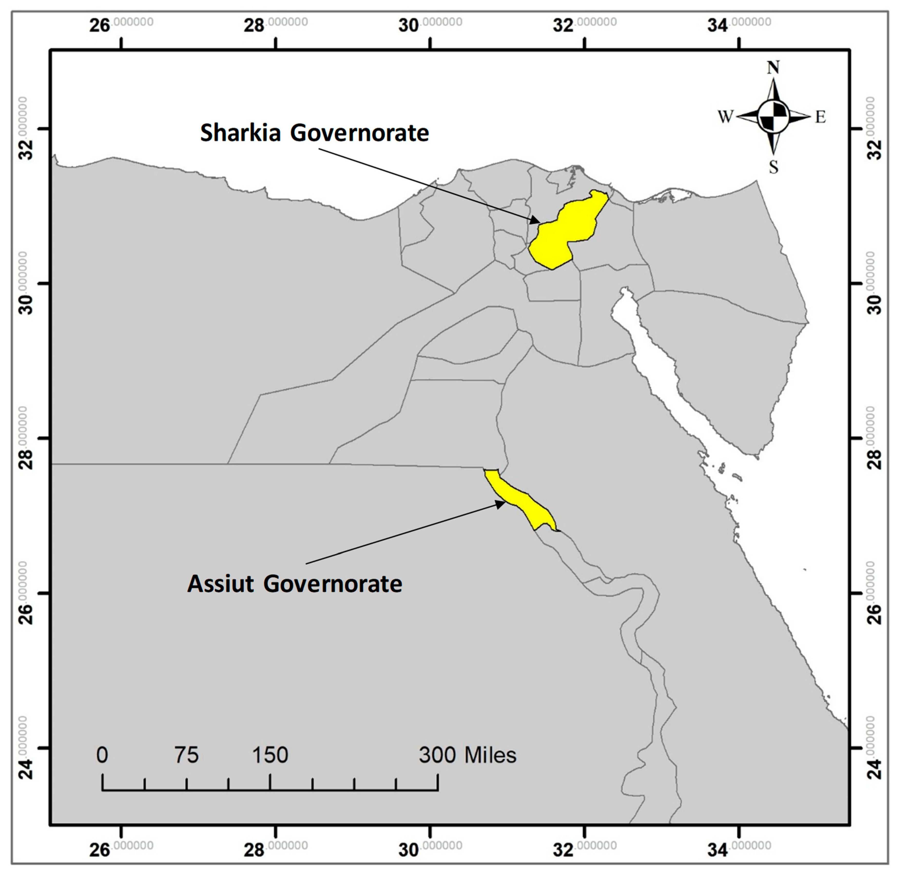
2.1. Study Areas and Data Collection

The study was conducted in Sharkia (six districts) and Assiut (three districts) Governorates of Egypt (Figure 1). A random sample of 360 individual household farms was selected from existing household farm lists of several districts in the two governorates: 180 household farms practicing traditional farming methods and the remaining 180 were adopters of MRBT.

In the surveyed household farms, the main crops grown in the summer season are rice (57% of the total summer cropping area, found only in Sharkia), maize (49%), cotton (26%, only in Sharkia), and sorghum (51%, only in Assiut). The main winter crops are wheat (91%) and clover (9%).

Surveyed traditional household farms in Sharkia Governorate comprise 14 from Zagazig, 30 from Awlad Saqr, five from Menia Al-Qamh, 15 from Hehia, 21 from Abo-Ahmed, and five from the Faqos district. The surveyed adopters of MRBT in Sharkia include 14 from Zagazig, 29 from Awlad Saqr, five from Menia Al-Qamh, 15 from Hehia, 20 from Abo-Ahmed, and seven from the Faqos district. In Assiut Governorate, the surveyed traditional farmers include 45 from Manfalot and 45 from the Al-Fat’h district, all of which are small farmers (100%). The surveyed MRBT adopters in Assiut comprise 60 from Al-Fat’h district and 30 from Abnob district. In addition, 19%, 64%, and 17% of them own land on the head, middle, and tail of Mesqa, respectively [23].

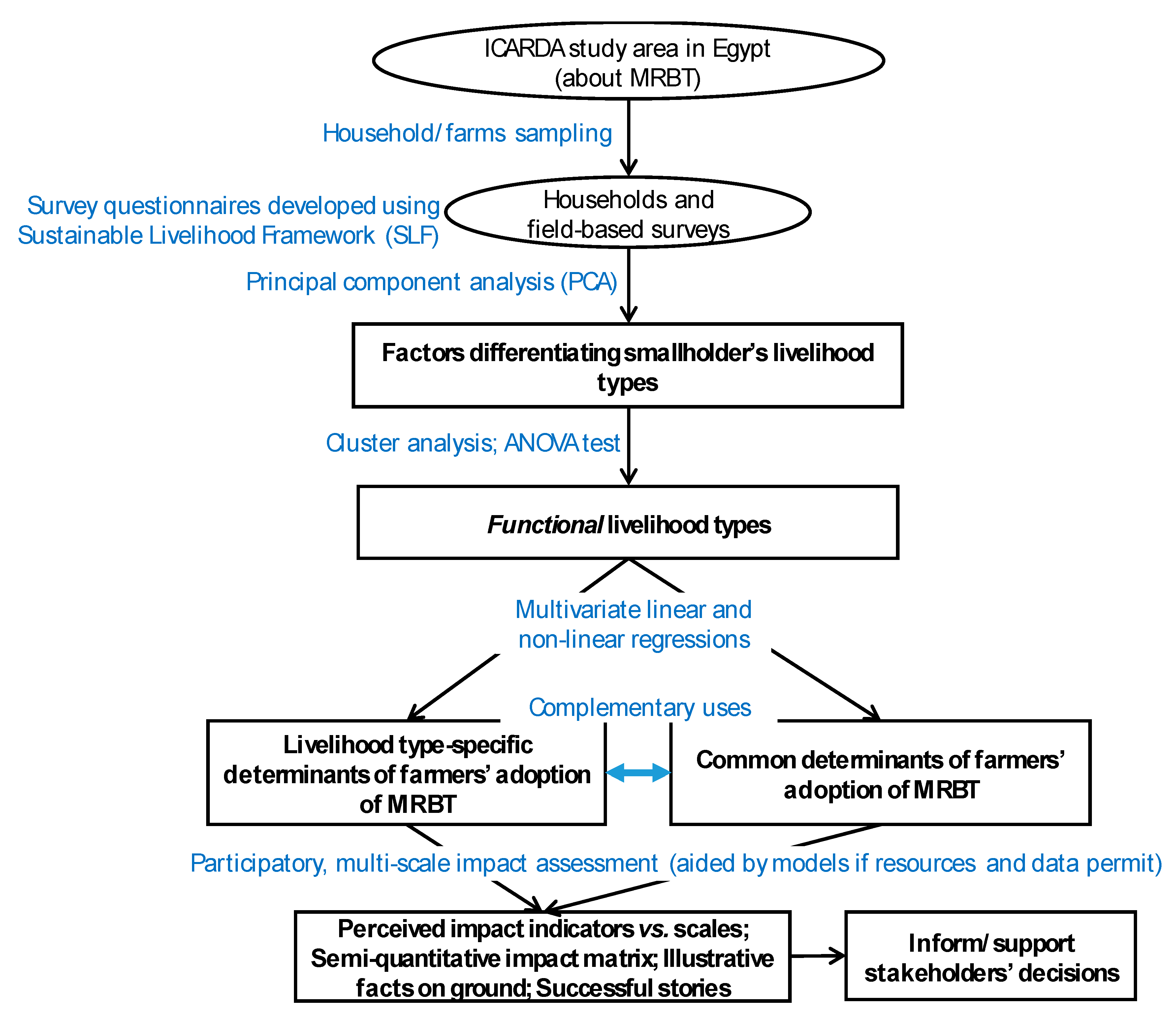
2.2. Analytical Framework

The analytical framework of agricultural livelihood typology-based approach proposed by [24] is applied. This framework includes sequential steps of empirical analyses toward achieving the stated objectives (Figure 2).

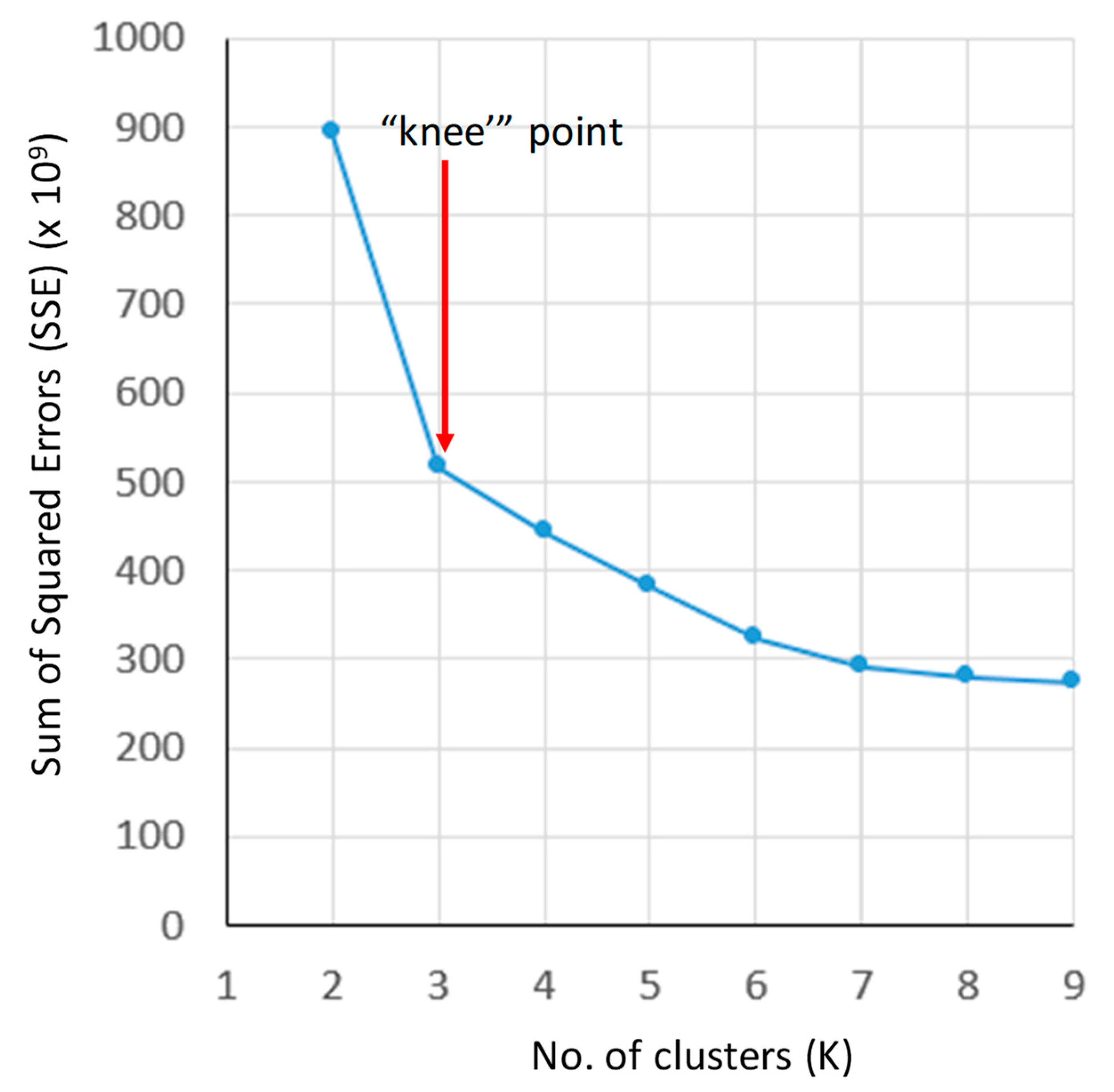
2.3. Methods for Identifying Livelihood Typology of Smallholder Farming Systems

Livelihood typology of smallholder farming systems is built on the concept of household/farm livelihood sustainability, including its adaptability and resilience in the vulnerability context. The sustainable livelihoods framework describes the essential resources and capabilities at household/farm disposal and livelihood strategies built from these resources in coping with the vulnerability context [25]. These resources comprise five types of livelihood assets that are used to achieve the households’ or community’s livelihood outcomes. Human assets include variables of labor, health, education, and capabilities. Natural assets comprise attributes of land (amount and quality), livestock, and water resources. Financial assets include incomes, savings, and loans from different sources. Physical assets consist of variables for housing conditions, access to infrastructure, and equipment for agricultural production. Social assets include supports and advantages from social networks (both in vertical and horizontal connections), engagement with rural development institutions, positions, and projects/programs. In addition, from the resilience approach, the five livelihood assets interactively determine the buffering capacity of livelihood systems. The adaptability and transformability of a household’s livelihood strategies will also be determined by its community’s institution for self-organizing and learning capacities [26]. This livelihood framework was used to guide the development of the content of questionnaires for livelihood surveys and indicators for analyses and assessments.

Table 1. Variables representing five livelihood assets considered in principal component analysis.

No.	Variable	Definition
	Human assets
1	H_AGE_HEAD	Age of the household head (years)
2	H_AGE_MEAN	Average age of household members (years)
3	H_EDU_HEAD	Education level of the household head (1 = illiterate, 2 = can read and write, 3 = secondary school, 4 = higher education)
4	H_HH_SIZE	Household size (no. of household members)
5	H_LABOR	Number of workers based on age (15–64 years old)
6	H_DEPEND_RATIO	Dependency ratio (no. of dependents/no. of workers)
	Natural assets
7	P_FARM_SIZE	Farm size, i.e., area of household farm (ha)
8	H_AREA_PERS	Farm area per capita (ha/household member)
9	P_SOIL_SALINITY	Severity of soil salinity perceived by the household (1 = low, 2 = moderate, 3 = high)
10	P_WATER_TABLE	Severity of water table raising perceived by the household (1 = low, 2 = moderate, 3 = high)
11	H_LIVESTOCK	Value of household’s livestock (EGP)
12	H_LIVESTOCK_PERS	Value of livestock per capita (EGP/household member)
13	H_POULTRY	Value of household’s poultry (EGP)
14	H_SMALL_RUMINANT	Value of household’s small ruminants (EGP)
15	H_CATTLE	Value of household’s cattle (EGP)
	Financial assets
16	H_INCOME	Annual income of household (EGP/year)
17	H_INCOME_PERS	Annual income per capita (EGP/household member year)
18	H_AGR_INCOME	Share of agricultural income (%)
19	H_NAGR_INCOME	Share of non-agricultural income (%)
20	H_LOAN_ACCESS	Household’s accessibility to loans, approximated by total loan value (EGP)
	Physical assets
21	P_DISTANCE_HOUSE	Distance from household farm to house (m)
22	P_DISTANCE_TOWN	Distance from household farm to nearest urban center (m)
23	H_NFLOORS	Number of house floors
24	H_NROOMS	Number of house rooms
25	H_EQUIPMENTS	Value of household’s equipment (EGP)
	Social assets
26	H_AC_EFFECTIVE	Effectiveness of agricultural cooperatives for the household as perceived (0 = ineffective, 1 = do not know (likely little effective), 2 = fairly effective, 3 = effective)
27	H_WUA_EFFECTIVE	Effectiveness of water use associations (WUA) for the household as perceived (four levels as for H_AC_EFFECTIVE)
28	H_AMA_EFFECTIVE	Effectiveness of agricultural market association for the household as perceived (four levels as for H_AC_EFFECTIVE)
29	H_AMA_MEMBER	Membership of agricultural market/marketing association (1 = have a membership, 0 = otherwise)
30	H_SDA_EFFECTIVE	Effectiveness of service development association for the household as perceived (four levels as for H_AC_EFFECTIVE)

Note: 1 EGP = 0.059 US$ (average exchange rate for 2019).

defines quantitative variables, which were specified using the sustainable livelihoods framework, for statistical analyses toward identifying livelihood types.

First, the principal component analysis (PCA) procedure wasused for discovering key factors explaining the majority of variation in the multivariate livelihood data, as well as reducing dimensionality of the data [27]. The meaning of each principal component (PC) is interpreted in terms of the original variables with higher weights/loadings. Because the extracted PCs are independent of each other, the use of component scores for subsequent analysis avoids the multi-collinearity problem that some explanatory variables are correlated and can cause problems for the interpretation of a regression model. There are 30 variables entered in PCA in this study (Table 1). Next, K-mean cluster analysis (K-CA) was used for deriving typical household/farm groups defined by livelihood criteria. K-CA is a multivariate statistic method that groups similar objects into groups called clusters. The endpoint of this cluster analysis is a set of clusters, where each cluster is distinct from each other cluster, and the objects within each cluster are broadly similar to each other. Unlike hierarchical clustering methods, the K-CA method avoids problems of chaining and artificial boundaries and works on the original input data rather than on a similarity matrix. For a large dataset (e.g., hundreds of cases), K-CA should be chosen because it would be difficult to interpret grouping results using hierarchical cluster analysis given that the considered sample is large [28]. Data entered into K-CA can be the scores of PCs extracted by the earlier PCA, or original livelihood variables that are highly correlative with the extracted PC.

To determine the number of clusters, a previously described procedure was used [29]. The optimal cluster number is defined as the minimal cluster number with the highest cluster homogeneity. First, K-CAs are run with the number of clusters set to all values K = 2, 3 …, 10. For each K-CA (with a concrete K-value), the mean distance of cases to their assigned cluster centers was calculated. These mean distance values were then plotted against the increasing cluster number (K = 2, 3 …, 10). The optimal cluster number was chosen by examining the “knee” of the curve: The point from which the overall cluster quality, i.e., the reduction of the mean distance from cases to their cluster centers, or the overall cluster homogeneity is not substantially improved when K increases [30]. The livelihood groups of households/farms defined at this stage are just potentially functional livelihood types. Livelihood types will be functional regarding MRBT adoption outcome if MRBT adoption rates and drivers differ among the livelihood types. The functional livelihood types are tested in adoption assessment in the next step.

2.4. Methods for Adoption Assessment

2.4.1. Dependent Variables

The first dependent variable used for inferential statistics (binary logistic regression) is the existence of MRBT practice in household-farms (MRB_PRACTICE). This is a straightforward (yes/no) adoption that is often seen in many publications.

The second dependent variable used for inferential statistics [multiple linear regression (MLR)] is the composite index of adoption quality that is conceptualized in the following formula:

$$AQ={{\displaystyle \prod }}_i^N{P}_i\times {{\displaystyle \sum }}_j^M{Q}_j,$$

(1)

where AQ is the adoption quality index, P_i is an on/off controlling factor of for AQ, and Q_j is quality attributes for the performance and/or impact of the practice of considered technology. In this study, P_i is the existence of a MRBT practice: If there is no MRBT practice (P_i = 0), then AQ = 0 regardless of Q_j value. We collected Q_j on farmers’ reflections on different benefits of MRBT, including improvements of household’s machinery ability (MRB_MA), technical knowledge and skills (MRB_KT), cost of adoption (MRB_AC), crop yield (MRB_YD), water saving (MRB_WS), marketability (MRB_MKA), and market price received (MRB_MKP). The short definitions of these adoption quality components are displayed in

Table 2. Variables representing different quality attributes of mechanized raised-bed technology (MRBT) adoption (i.e., adoption quality attributes) as dependent variables in regression analysis for identifying adoption’s determinants.

Adoption Quality Attribute	Definition	Unit (Range)
MRM_PRACTICE	Existence of MRBT practice	0 = traditional farm, 1 = MRBT practiced
MRB_MA	Self-reflection of MRBT’s benefit in improving household’s machinery ability	0 = no difference created by MRBT, 1 = do not know (not clear), 2 = better
MRB_KT	Self-reflection of MRBT’s benefit in improving household’s knowledge and technology	0 = no difference created by MRBT, 1 = do not know (not clear), 2 = better
MRB_AC	Self-reflection of MRBT’s benefit in reducing household’s cost of adoption	0 = no difference created by MRBT, 1 = do not know (not clear), 2 = better
MRB_YD	Self-reflection of MRBT’s benefit in improving farm’s crop yield	0 = no difference created by MRBT, 1 = do not know (not clear), 2 = better
MRB_WS	Self-reflection of MRBT’s benefit in improving farm’s water saving	0 = no difference created by MRBT, 1 = do not know (not clear), 2 = better
MRB_MKA	Self-reflection of MRBT’s benefit in improving household’s market ability	0 = no difference created by MRBT, 1 = do not know (not clear), 2 = better
MRB_MKP	Self-reflection of MRBT’s benefit in improving market price received	0 = no difference created by MRBT, 1 = do not know (not clear), 2 = better
AQ	Adoption quality index (AQ) of MRBT, i.e., a product of MRBT implementation with the sum of score reflecting MRBT’s benefits (see Equations (1) and (2))	Score between 0 and 14

. Therefore, in this study, the equation for AQ takes the following form:

AQ = MRB_PRACTICE × (MRB_MA + MRB_KT + MRB_AC + MRB_YD + MRB_WS + MRB_MKA + MRB_MKP)

(2)

2.4.2. Inferential Statistical Models

For the MRB_PRACTICE, because it is in binary scale (1 if the household practices MRBT and 0 otherwise, i.e., traditional farm), binary logistic regression (bi-logit) is used to identify factors determining MRBT adoption. As site-specific constraints and potentials influence MRBT outcomes, the unit of MRBT adoption analysis is recommended to be a field rather than a household. The effect of the hypothesized socio-ecological variables on the adoption of MRBT by a household can be modeled as:

P(MRBT) = 1/(1 + exp (β₀ + β₁X₁ + β₂X₂ + β₃X₃ + … + β_nX_n + µ))

(3)

where P(MRBT) is the probability of MRBT adoption. X_i and β_i (i = 1, 2, 3, …, n) are explanatory variables and their weight coefficients (or affecting coefficients), respectively, and µ is a random error term.

Performance evaluation of binary logistic regressions includes:

• Chi-squared test for overall statistical significance of the regression model (Hosmer–Lemeshow test);
• Probability of correct prediction, and;
• Receiver Operating Characteristic (ROC) statistics.

Although the pseudo-coefficient of determination (pseudo-R²) in bi-logit mimics the widely used R² in linear regression, there are no agreed benchmark values of pseudo-R² for determining whether model performance is acceptable. As an alternative, the goodness-of-fit of the model uses ROC statistics, as recommended by several experts in binary logistic regressions [31,32,33]. The ROC curve depicts the model sensitivity (true positive fraction) and model specificity (true negative fraction) over all possible cut-off points. The area under the ROC curve (theoretically ranging within 0.5–1) is used as the basis for evaluating model performance. If the area value is significantly (p < 0.05) higher than 0.5, then the model predicts the output better than chance. Area values of 0.7–0.8 show acceptable model performance, values of 0.8–0.9 demonstrate excellent performance, and values >0.9 indicate outstanding performance [31].

From another side, MLR is used for inferring determinants of AQ. Performance of MLR models is measured by F-test and R².

2.4.3. Explanatory Variables

The vector of explanatory variables [X_i] (i = 1, 2, 3, …, n) is from the indicators of livelihood assets of the household that owns or operates the land. Vector [X_i] can have some overlap with the variables in the earlier PCA, but not necessarily. In general, inclusion of livelihood variables in [X_i] should be based on an understanding (through either literature or common sense) of the rationales of their effects on adoption of MRBT. The explanatory variables for regression analyses in this study are shown in

Table 3. Explanatory variables considered in regression analyses for identifying determinants of MRBT adoption.

No.	Variable	Definition	Hypothesized Effect
	Human asset
1	H_AGE_HEAD	Age of the household head (years)	−
2	H_AGE_MEAN	Average age of household members (years)	-
3	H_EDU_HEAD	Education level of the household head (unit: See Table 1)	+
4	H_HH_SIZE	Household size (no. of household members)	-/+
5	H_LABOR	Number of workers based on age (15–64 years old)	-
6	H_DEPEND_RATIO	Dependency ratio (no. of dependents/no. of workers)	-/+
	Natural asset
7	P_FARM_SIZE	Farm size, i.e., area of household farm (ha)	+
8	H_AREA_PERS	Farm area per capita (ha/person)	+
9	P_SOIL_SALINITY	Severity of soil salinity (unit: See Table 1)	+
10	P_WATER_TABLE	Severity of water table raising (unit: See Table 1)	+
11	H_LIVESTOCK_PERS	Value of livestock per capita (EGP/person)	+/-
12	H_POULTRY	Value of household’s poultry (EGP)	+/-
13	H_GOAT	Value of household’s goats (EGP)	+/-
14	H_SHEEP	Value of household’s sheep (EGP)	+/-
15	H_BUFFALO	Value of household’s buffaloes (EGP)	-
16	H_COW	Value of household’s cows (EGP)	+/-
	Financial asset
17	H_INCOME	Annual income of the household (EGP/year)	+/-
18	H_INCOME_PERS	Annual income per capita (EGP/person/year)	+/-
19	H_INCOME_AGR	Annual income from agriculture (EGP/year)	+/-
20	H_INCOME_NAGR	Annual income from non-agricultural sources (EGP/year)	+/-
21	H_LOAN_ACCESS	Household’s accessibility to loans (EGP)	+
	Physical asset
22	P_DISTANCE_HOUSE	Distance from household farm to house (m)	-
23	P_DISTANCE_TOWN	Distance from household farm to nearest urban center (m)	-
24	H_NFLOORS	Number of house floors	+/-
25	H_NROOMS	Number of house rooms	+/-
26	H_EQUIPMENTS	Value of household’s equipment (EGP)	+/-
	Social asset
27	H_AC_EFFECTIVE	Effectiveness of agricultural cooperatives (unit: See Table 1)	+
28	H_WUA_EFFECTIVE	Effectiveness of Water Use Association (WUA) (unit: See Table 1)	+
29	H_AMA_EFFECTIVE	Effectiveness of agricultural market/marketing association (unit: See Table 1)	+
30	H_AMA_MEMBER	Membership of agricultural market/marketing association (unit: See Table 1)	+
31	H_SDA_EFFECTIVE	Effectiveness of service development association (unit: See Table 1)	+

.

Both regression models require the checking of multi-collinearity problems that the explanatory variables can cause for the regression models. High multi-collinearity (i.e., strong linear relationship among two or more explanatory variables) is a problem because it undermines the statistical significance of an independent variable. Before conducting regression analyses, we tested for multi-collinearity of all explanatory variables using Variance Inflation Factors (VIF). Ideally, there will be serious collinearity problems for VIF > 5 [34]. We remove explanatory variables of VIF > 10 to reduce serious multi-collinearity [35]. All statistical analyses were done using SPSS 16.

3. Results and Discussion

3.1. Identified Agricultural Livelihood System (ALS) Types

3.1.1. Factors Explaining the Differences in ALS Types

The PCA run extracted nine principal components with total eigenvalues greater than 1.0, explaining 74% of the total variance of the 30 original livelihood variables. The rotated component matrix then helped to determine what the components represent (

Table 4. Extracted principal components (PCs), loading coefficients of variables vs. PCs, and key variables (with bolded names and loadings).

Variable	PC1 (Market—13.4%)	PC2 (Agr. Income—11.7%)	PC3 (Livestock—11.3%)	PC4 (Labor—9.5%)	PC5 (Age—7.2%)	PC6 (Non-Agri. Income—6.5%)	PC7 (House Quality—6.4%)	PC8 (Access-to-Farm—4.3%)	PC9 (Less Access-to-Loans—3.9%)
H_AGE_HEAD	0.052	0.220	0.119	0.652	0.554	0.063	0.085	0.075	0.150
H_AGE_MEAN	−0.010	0.122	0.042	0.027	0.889	−0.010	−0.038	0.069	0.076
H_EDU_HEAD	0.369	−0.078	−0.139	−0.358	−0.225	0.134	0.334	−0.280	−0.032
H_HH_SIZE	0.188	0.213	0.150	0.856	−0.191	0.071	0.129	−0.039	0.074
H_LABOR	0.222	0.009	0.142	0.806	0.268	0.050	0.171	−0.084	−0.098
H_DEPEND_RATIO	−0.142	0.164	−0.047	0.017	−0.807	0.038	−0.073	0.050	0.212
P_FARM_SIZE	0.153	0.157	0.462	−0.039	0.145	0.000	0.128	0.021	0.562
H_AREA_PERS	−0.060	−0.021	0.351	−0.666	0.349	−0.028	−0.004	0.019	0.423
P_SOIL_SALINITY	0.526	0.556	0.238	0.006	0.091	−0.162	0.092	0.091	−0.066
P_WATER_TABLE	0.708	0.170	0.136	−0.162	0.004	−0.143	−0.011	0.260	−0.207
H_LIVESTOCK	0.151	0.212	0.906	0.201	0.010	−0.021	0.033	0.106	−0.019
H_LIVESTOCK_PERS	0.029	0.001	0.823	−0.238	0.136	−0.014	−0.059	0.077	0.001
H_POULTRY	0.266	0.356	0.342	0.141	0.013	0.166	0.154	−0.053	−0.086
H_SMALL_RUMINANT	0.167	0.450	0.552	0.149	−0.093	0.041	0.088	−0.041	0.032
H_CATTLE	0.116	0.106	0.892	0.187	0.036	−0.045	0.006	0.138	−0.025
H_INCOME	0.136	0.722	0.105	0.120	−0.022	0.578	0.122	−0.022	−0.029
H_INCOME_PERS	0.074	0.623	0.046	−0.043	0.041	0.703	0.079	−0.032	−0.063
H_AGR_INCOME	0.187	0.858	0.173	0.118	0.008	−0.062	0.011	0.047	0.008
H_NAGR_INCOME	0.047	−0.117	−0.082	0.068	−0.054	0.897	−0.025	0.022	−0.069
H_LOAN_ACCESS	0.028	0.063	0.128	0.025	0.123	0.074	−0.074	−0.008	−0.605
P_DISTANCE_HOUSE	0.005	−0.089	0.155	−0.167	−0.028	−0.050	0.259	0.782	−0.051
P_DISTANCE_TOWN	0.882	0.230	0.084	0.059	0.018	0.047	−0.139	0.075	−0.104
H_NFLOORS	−0.156	0.107	0.026	0.146	0.037	0.009	0.856	0.084	0.080
H_NROOMS	−0.272	0.137	0.058	0.123	0.036	0.000	0.839	0.092	0.098
H_EQUIPMENTS	0.309	0.330	0.196	0.237	0.156	0.128	−0.109	0.458	0.231
H_AC_EFFECTIVE	0.488	0.098	0.078	0.209	0.088	0.354	−0.166	0.439	0.119
H_WUA_EFFECTIVE	0.216	0.841	0.082	0.079	0.017	−0.022	0.076	−0.004	0.054
H_AMA_EFFECTIVE	0.744	0.128	0.147	0.156	0.043	0.220	−0.116	−0.102	0.152
H_SDA_EFFECTIVE	0.609	0.121	0.014	0.121	0.026	0.010	−0.025	0.022	0.007
H_AMA_MEMBER	0.774	0.090	0.133	0.175	0.063	0.054	−0.228	−0.095	0.166

Note: Cells marked in green and with bold letters are key variables in explaining the principal factors (PCs).

). The PC1 was strongly related to variables approximating access/connection to market, both physical market access (H_DISTANCE_TOWN) and institutional market connection (H_AMA_EFFECTIVE and H_AMA_MEMBER). Thus, this component was named “Market factor”, and explained 13.4% of total variance of the original dataset. The PC2 was most weighted by income variables, especially the share of income from agriculture (H_AGR_INCOME). Therefore, we labeled this “Agricultural income factor” and it accounted for 11.7% of total variance of the original dataset. The PC3 accounted for 9.5% of total variation and was most highly correlated with three livestock variables—H_LIVESTOCK, H_LIVESTOCK_PERS, and H_CATTLE—and, thus, was called the “Livestock factor”. Pairwise correlations of the three variables showed that they were strongly correlated. Because of the high loading value, H_LIVESTOCK was selected to represent the Livestock factor. The PC4 was highly correlated with the demographic variables of surveyed household (H_SIZE and H_LABOR) and demographic pressure on land (H_AREA_PERS), and was called the “Labor factor”.

The PC5 was explained mainly by the variable of family mean age (H_AGE_MEAN) and dependency ratio (H_DEPENRATIO) was called the “Age factor”. The PC6 was mainly related to the share of on-agricultural income (H_NAGR_INCOME), thus named “Non-agricultural income factor”. The PC7 was strongly associated with variables indicating house quality (H_NFLOORS and H_NROOMS), thus referred to as “House quality factor”. The PC8 was mainly explained by distance from household house to farm, reflecting the household’s physical transaction cost in daily farming, thus named “Access-to-farm factor”. The PC9 was inversely related to household access to loans (H_LOAN_ACCESS), thus called “Less access-to-loans factor”. However, as PC9 accounted for only 4% of the total data variation, and the loading of H_LOAN_ACCESS was not high, the role of this variable for distinguishing ALS types may not be important.

3.1.2. ALS Types

Twenty-two variables with loading >0.6 in Table 4 were used for subsequent cluster analyses (K-CA). We ran eight K-CA with K = 2, 3, …, 10 that used these 22 variables, and calculated the sum of squared errors (SSE) for every K-CA run. Figure 3 depicts the distribution of SSE versus the running number of clusters (K), which shows a “knee” point at K = 3, suggesting an optimal cluster number of K = 3 for the final K-CA. Increasing the cluster number further from this point will not effectively increase the average clumsiness of each cluster (clustering quality inversely approximated by SSE) [36].

The final K-CA with K = 3 resulted in three clusters of farm-households. An ANOVA was used to test the differences among the mean values of the 22 used variables (data not shown). The final selection of a limited set of variables for characterizing the clusters was based on the statistical differences via ANOVA tests. In many variables, although there were significant differences among their mean values across ALS types, the variables were not picked to characterize the clusters because the mean differences were either less or equal to only one measuring unit of the variables (e.g., the case of H_SIZE, H_LABOR, H_NFLOORS, and H_NROOMS). Some variables had significantly high correlations with each other. In these cases, the most meaningful variable of them was selected. The key variables for characterizing ALS types are shown in

Table 5. Key characteristics of three potential Agricultural Livelihood System (ALS) types.

Livelihood Asset Category	Key Variable (Abbreviation)	$\overline{\mathit{X}}\pm \mathit{C}{\mathit{I}}_{0.05} (\mathbf{Mean} \text{±} \mathbf{Confidence} \mathbf{Interval} \mathbf{at} 95\%)$
		ALS Type I (n = 196) (Poor and Non-Agriculture-Based Income)	ALS Type II (n = 96) (Medium and Balanced Crop–Livestock–Non-Farm Income)	ALS Type III (n = 61) (Medium, Less Dependent Pressure, Livestock/Cattle-Based Income)
Human	H_AGE_MEAN	31 ± 1	31 ± 1	34 ± 2
	H_DEPENRATIO	0.39 ± 0.07	0.40 ± 0.10	0.30 ± 0.07
Natural	H_AREA_PERS (m2/person)	1442 ± 213	1176 ± 116	2170 ± 519
	H_LIVESTOCK (100 EGP)	41 ± 14	878 ± 44	16,445 ± 74
Financial	H_INCOME_PERS (100 EGP/person)	19 ± 6	34 ± 10	35 ± 11
	H_AGR_INCOME (%)	3 ± 2	29 ± 9	35 ± 12
	H_NAGR_INCOME (%)	23 ± 6	18 ± 8	11 ± 7
Physical	P_DISTANCE_HOUSE (m)	830 ± 138	1278 ± 241	1236 ± 324
	P_DISTANCE_TOWN (m)	3421 ± 539	5798 ± 685	5444 ± 802
Social	H_AMA_EFFECTIVE 1	1	3	1
	H_AMA_MEMBER 1	0	1	1

¹ Median is used instead of metric mean for variables measured in Likert scale.

.

ALS type 1 (n = 196, 55%): Poor household-farms (1900 EGP (EGP = 0.059 US$ as an average exchange rate for 2019)/person/year) with main income based on non-agricultural activities at low cost (agricultural income being 3% of the total income), less access to local market institutions such as agricultural market associations (AMA). It is likely these household members have frequent low-cost non-farm activities in town as they live closer to urban centers (3.7 km) compared to the two other ALS types (5.5–5.8 km).

ALS type 2 (n = 96, 27%): Medium household-farms (3400 EGP/person/year) with balanced crop–livestock–non-farm income, being sensitive/positive to role of local market institutions (e.g., AMA) compared to other ALS types.

ALS type 3 (n = 61, 17%): Medium household-farms (3500 EGP/person/year) with livestock/cattle-based income, and less pressure from independent household members.

3.2. Determinants of MRBT Adoption

3.2.1. Adoption Responses versus ALS Types

The MRBT adoption practice, adoption quality attributes, and AQ versus ALS types are shown in

Table 6. MRBT adoption practice, adoption quality attributes, and composite adoption quality index (AQ) versus ALS types.

Adoption Variable	Category	ALS Type 1	ALS Type 2	ALS Type 3	Whole Sample
MRBT practice (MRB_PRACTICE)	0 = Traditional farm	98	45	32	175
	1 = MRBT practiced farm	98	51	29	178
	% MRBT practiced	50	53	48	50
Self-reflection of MRBT’s benefit on household’s machinery ability (MRB_MA)	0 = No difference	3	2	0	5
	1 = Do not know	62	27	18	107
	2 = Better	131	67	43	241
	% Better	67	70	70	68
Self-reflection of MRBT’s benefit on improved knowledge and technology (MRB_KT)	0 = No difference	22	8	4	34
	1 = Do not know	169	77	53	299
	2 = Better	5	11	4	20
	% Better	3	11	7	6
Self-reflection of MRBT’s benefit on adoption cost (MRB_AC)	0 = No difference	8	10	6	24
	1 = Do not know	72	32	20	124
	2 = Better	116	54	35	205
	% Better	59	56	57	58
Self-reflection of MRBT’s benefit on crop yield (MRB_YD)	0 = No difference	1	1	1	3
	1 = Do not know	64	28	18	110
	2 = Better	131	67	42	240
	% Better	67	70	69	68
Self-reflection of MRBT’s benefit on water saving (MRB_WS)	0 = No difference	1	2	1	4
	1 = Do not know	65	28	18	111
	2 = Better	130	66	42	238
	% Better	66	69	69	67
Self-reflection of MRBT’s benefit on household’s marketability (MRB_MKA)	0 = No difference	22	8	4	34
	1 = Do not know	169	77	53	299
	2 = Better	5	11	4	20
	% Better	3	11	7	6
Self-reflection of MRBT’s benefit on market price received (MRB_MKP)	0 = No difference	22	9	4	35
	1 = Do not know	171	76	53	300
	2 = Better	3	11	4	18
	% Better	2	11	7	5
MRBT adoption quality (AQ) index (mean value)		5.1	5.6	4.9	5.2

. The adoption quality attributes responsive to ALS types include farmers’ reflection on MRBT benefits on technical knowledge and skills (MRB_KT), marketability (MRB_MKA), and market price received (MRB_MKP). The other adoption attributes did not respond differently to diverse ALS types, in which household-farms of ALS type 2 were most positive in MRBT adoption for these three quality attributes.

3.2.2. Determinants of MRBT Adoption (Yes/No Adoption)

The results of binary logistic regression for identifying determinants of MRBT practice adoption for the whole sample population and three ALS types are presented in

Table 7. Results of regression analyses (binary logistic model) identifying determinants of the MRBT implementation (MRB_PRACTICE).

Explanatory Variable	Weigh/Affecting Coefficient (βi)
	Whole Population (n = 353)	ALS Type 1 (n = 196)	ALS Type 2 (n = 96)	ALS Type 3 (n = 61)
Intercept	4.16723 **	−3.112025	2.795705	535.074263
H_AGE_HEAD	0.036484	−0.023694	0.259528 *	3.670878
H_AGE_MEAN	−0.059180 *	−0.036237	−0.277310 *	−4.258127
H_EDU_HEAD	0.336165 *	0.100004	0.533685	−0.345585
H_HH_SIZE	0.085064	0.205301	−1.837035	4.877359
H_LABOR	−0.485084	−0.648082	0.896835	−18.400223
H_DEPRATIO	−1.352001	−2.185917	1.739649	−92.624210
P_FARM_SIZE	0.556649	2.511402 *	9.995974	−83.072594
H_FARM_PERS	1.223084	−1.811349	−50.953806	97.441248
P_SALINITY	−0.127766	−0.666194	0.595789	−50.489758
P_WATER_TABLE	−0.632814 *	−0.360940	−0.221991	−100.267632
H_LIVESTOCK_PERS	−0.000019	0.001005	0.000280	−0.000676
H_POULTRY	0.000093	0.000037	−0.000050	0.002230
H_GOAT	−0.000005	−0.000424	−0.000120	−0.000134
H_SHEEP	0.000077 ***	−0.000061	0.000052	0.000307
H_BUFFALO	0.000003	−0.000199	−0.000097	−0.001048
H_COW	0.000008	−0.000178	−0.000045	−0.000071
H_INCOME	0.000036 *	0.000096 ***	0.000022	−0.003875
H_INCOME_PERS	−0.000019	−0.000204 *	0.000010	0.008142
H_INCOME_AGR	−0.000046 **	−0.000466	−0.000042	0.002547
H_LOAN_ACCESS	−0.000004	−0.001434	0.000007	−0.006201
P_DISTANCE_FARM	−0.000488 **	−0.000632	−0.000619	−0.012088
P_DISTANCE_TOWN	0.000060	0.000016	0.000078	0.009058
H_NFLOORS	−0.647272 **	−0.928635 *	−0.618283	8.672878
H_NROOMS	0.300600 ***	0.434100 ***	0.343082 *	−4.747966
H_EQUIPMENT	−0.000137 ***	−0.000144 ***	−0.000197 ***	−0.005918
H_AC_EFFECTIVE	0.220648	0.215050	1.478817	13.781440
H_WUA_EFFECTIVE	−0.192171	9.892515	−0.885360	48.918104
H_AMA_EFFECTIVE	−0.107161	0.271273	−1.004542	15.627895
H_AMA_MEMBER	1.743556 ***	1.116570	3.589761 **	−20.984578
H_SDA_EFFECTIVE	0.097971	−0.087460	−0.045027	27.589114
Model performance
Hosmer–Lemeshow test	Chi-square = 8.478, df = 8, p = 0.388	Chi-square = 12.455 df = 8, p = 0.132	Chi-square = 20.574, df = 8, p = 0.08	Chi-square = 0.000 df = 8, p = 1.000
Correct prediction	75.6%	77.0%	80.2%	100%
Area under ROC	0.85 (p < 0.001)	0.69 (p < 0.001)	0.70 (p < 0.001)	0.61 (p < 0.001)

Notes: Symbols *, **, and *** indicate a statistical significance at 90% (p < 0.1), 95% (p < 0.05), and 99% (p < 0.01), respectively.

. For whole sampled population and sub-groups of ALS types 1 and 2, the Hosmer and Lemeshow tests for the bi-logit models showed acceptable results: p > 0.05 showed no significant difference between predicted data for MRBT adoption and observed data, meaning that there was a good fit of the model to the data used. The percentage of overall correct predictions of the models were relatively high (76–80%). The calculated area under the ROC curve ranged within 0.69–0.85, indicating that performance of the models varied from acceptable to excellent for identifying the determinants of MRBT adoption. Although there was no sign of failure in the parameters of model performance tests, the bi-logit model for ALS type 3 had no explanatory power, with no variable demonstrating a significant effect. The poor statistical performance of ALS type 3 may be due to the small size of this farm cluster (n = 61) compared to a long list of used explanatory variables (30 variables).

Table 7 shows 14 variables with a significant effect on MRBT adoption. These 14 determinants of MRBT adoption can be of four categories:

Common determinants for MRBT adoption (two variables): Common determinants of adoption were the explanatory variables found significant for the whole population and individual ALS types, and sharing the same direction of effect. If all determinants were common, then the treatment of adoption analyses for individual ALS types would have no benefit. In Table 7, among the 14 variables with significant effects, only two variables within the physical asset category were common determinants: H_NROOMs (supporting MRBT adoption) and H_EQUIPTMENT (discouraging MRBT adoption).

ALS type-specific determinants for MRBT adoption—type 1 (four variables): A determinant for adoption in this type was an explanatory variable found significant for the whole population, and for one of a few individual ALS type(s) rather than all individual ALS. In this case, the added value given by the treatment of individual ALS was to further narrow the specific zone(s)/condition(s) where the effect actually took place. Determinants of this type included average age of the family (H_AGE_MEAN) and income (H_INCOME) which effects are happen in ALS type 2. Membership of agricultural market association (H_AMA_MEMBER) encouraged farmers to adopt MRBT in general, but the effect was further narrowed in ALS type 3 (the medium and livestock-based farmers).

ALS type-specific determinants for MRBT adoption—type 2 (three variables): Determinants for adoption in this type were explanatory variables found for one of a few individual ALS type(s) but not realized through analysis of the whole population, reflecting the added value given by the use of individual ALS types. There were four determinants for MRBT adoption of this type, including farm size (H_FARM_SIZE) and income per capita (H_INCOME_PERS), for which effects are found only in ALS type 1 (poor and low-cost non-agriculture based). With larger farm size there was more adoption of MRBT in this group of farmers. This finding suggests that large farms should be targeted to widely spread adoption of MRBT. The negative effect of income per capita is understandable because the income of this group is largely based on non-agricultural activities. Here, the result of group characterization, as a step of the approach, eased the interpretation of the effect. A negative effect of the age of household head (H_AGE_HEAD) on MRBT adoption was found only in ALS type 3 (medium and livestock-based), but was statistically weak.

Determinants for MRBT adoption found only in whole-population analysis (five variables): The determinants of this category included five variables: Education of household head (H_EDU_HEAD) and sheep (H_SHEEP) with positive effects; and severity of water table raising (H_WATER_TABLE), share of agricultural income (H_INCOME_AGR), and distance from house to farm (H_DISTANCE_FARM) with negative effects. Except for H_INCOME_PERS, the effect directions of determinants agreed with common sense. The existence of determinants in this category demonstrates the complementary role of whole-population adaption analysis except for the ALS type specific ones.

3.2.3. Determinants of MRBT AQ

The empirical findings of the MLR analysis, with MRBT AQ as the dependent variable is shown in

Table 8. Results of regression analyses (multiple linear model) identifying determinants of the MRBT Adoption Quality (MRB_ADOPT_QUAL).

Explanatory Variable	Weight/Affecting Coefficient (βi)
	Whole Sample Population (n = 353)	ALS Type 1 (n = 196)	ALS Type 2 (n = 96)	ALS Type 3 (n = 61)
Intercept	12.031138 ***	8.0533050 ***	12.697623 **	21.784745 ***
H_AGE_HEAD	−0.042868	−0.0820910	0.023392	0.104024
H_AGE_MEAN	0.003843	0.0293595	−0.036492	−0.182747
H_HH_SIZE	0.699425	0.6011159	0.097752	−1.990863
H_FARM_PERS	1.098808	2.4674827	9.241878	2.672397
P_SALINITY	−0.082025	−0.6731696	−0.135969	−0.678263
P_WATER_TABLE	−0.700973	−0.4258870	−0.662324	−1.458162
H_POULTRY	0.000067	0.0001706	−0.000077	−0.000006
H_GOAT	0.000004	−0.0001065	−0.000116	0.000025
H_SHEEP	0.000124 ***	0.0000202	0.000163 **	0.000099 **
H_BUFFALO	−0.000003	0.0000396	−0.000048	−0.000019
H_COW	0.000004	0.0000136	−0.000007	−0.000020
H_INCOME_AGR	−0.000007	−0.0001021	−0.000011	0.000006
H_INCOME_NAGR	0.000055 ***	0.0000649 ***	0.000054	−0.000081
P_DISTANCE_FARM	−0.000617 **	−0.0005894	−0.000283	−0.000984
P_DISTANCE_TOWN	−0.000068	−0.0001804	0.000445	−0.000059
H_NFLOORS	−0.815685 **	−0.8750639	−0.855526	−0.549728
H_NROOMS	0.376476 ***	0.4222141 **	0.388385	0.125627
H_EQUIPMENT	−0.000205 ***	−0.0001949 ***	−0.000210 ***	−0.000253 ***
H_AC_EFFECTIVE	0.485688	0.4837751	0.785828	0.217742
H_WUA_EFFECTIVE	−0.175095	4.2093391 **	−1.467264	0.155717
H_AMA_EFFECTIVE	−0.509836	0.6123337	−1.508532 *	−1.035367
H_AMA_MEMBER	3.463651 ***	1.6777887	3.459019	4.216389
H_SDA_EFFECTIVE	0.099145	−0.4385565	−0.095141	1.003309
Model performance
F-test	F = 6.404 df = 23 p < 0.001	F = 4.275 df = 23 p < 0.001	F = 1.872 df = 23 p < 0.05	F = 3.209 df = 23 p < 0.001
Goodness-of-fit	R = 0.56 R2 = 0.31 adjusted-R2 = 0.26	R = 0.60 R2 = 0.36 adjusted-R2 = 0.28	R = 0.61 R2 = 0.37 adjusted-R2 = 0.17	R = 0.82 R2 = 0.67 adjusted-R2 = 0.46

Notes: Symbols *, **, and *** indicate a statistical significance at 90% (p < 0.1), 95% (p < 0.05), and 99% (p < 0.01), respectively.

. The list of explanatory variables used is shorter than those shown in Table 3 (Section 3.2) because variables with high VIF were excluded with the purpose to minimize the problem of multi-collinearity for MLR models. The F-tests indicated that all MLR models for explaining MRBT AQ significantly differed at confidence levels of 95% (p < 0.05) or 99% (p < 0.01).

Table 8 shows nine variables with a significant effect on AQ, which can be grouped into three main categories:

(1)

Common determinants for MRBT adoption (one variable): The common determinant of MRBT adoption quality was household equipment (H_EQUIPMENT)(significantly negative).

(2)

ALS type-specific determinants for MRBT adoption, with two types in this category:

-

Type 1 (three variables): Determinants of this type included the share of non-agricultural income (H_INCOME_NAGR) and number of rooms in house (H_NROOMS) that were further narrowed for ALS type 1. The effect of household sheep (H_SHEEP) (significantly positive) was common for the whole population and ALS types 2 and 3.

-

Type 2 (two variables): The strong positive effects of effectiveness of Water Use Association (WUA) (H_WUA_EFFECTIVE) on MRBT AQ were found only in ALS type 1. Without the ALS type-specific adoption analyses, this determinant—being meaningful for policy and management practice—would not have been realized. The negative effect of agricultural market association effectiveness (H_AMA_EFFECTIVE) on MRBT adoption quality was found only in ALS type 2, which is quite unusual and needs further interpretation with additional information.

(3)

Determinants for MRBT adoption found only in the whole-population analysis (three variables): The determinants of this category included distance from house to farm (H_DISTANCE_FARM), number of house floors (H_NFLOORS) (both significantly negative), and membership in agricultural market association (H_AMA_MEMBER) (significantly positive).

3.3. Evaluation of Added Values of the ALS Typology-Based Method Compared to Traditional Approach

Table 9. Evaluation of added values and limitations of the ALS typology-based method compared to traditional approach using evidence provided by this study.

Approach	Category of Determinants	Number of Determinants		Added Value	Limitation-Alternative
		MRBT Adoption (yes/no)	MRBT Adoption Quality (AQ Index)
Traditional approach: Use of sample-whole analysis only (business-as-usual)	Total determinants for MRBT adoption	10	7	Utilize large size of whole sample to increase statistical power	Findings do not necessarily reflect widespread effects
ALS typology-based approach: Complementary use of both ALS type-specific and whole-sample analyses (this study)	Common determinants across ALS types	2	1	Confirm widespread effects	Inferential statistical models for small ALS groups have poor performance, probably for two reasons: Small sample size reduces the power of parametric statistics. Alternative: Additional uses of non-parametric method for small ALS groups; ALS classification tends to reduce within-cluster variation, causing poor performance of statistical analysis if the same data of ALS grouping are used for adoption analysis. Alternative: Use additional data sources for adoption analysis.
	ALS type-specific determinants—category 1	4	3	Identify concrete household groups subjected to the effects found in whole-sample analysis
	ALS type-specific determinants—category 2	3	2	Discover new causal effects that cannot be done by traditional approach
	Determinants found only in whole-sample analysis	5	3	Utilize large size of whole sample to increase statistical power, thus off-setting the problem for the small ALS group
	Total determinants for MRBT adoption	14	9	Capture more quantity and comprehension of causalities in MRBT adoption

shows evaluation remarks on the added values and limitations of the ALS typology-based method compared to the traditional approach. The ALS typology-based approach, presented in this study, is the complementary use of both ALS type-specific and whole-sample analyses. The traditional approach, often found in current literature of adoption analysis, is the use of whole-sample analysis only. The evaluation remarks result from the findings of presented adoption analyses.

Overall, the ALS typology-based approach captured more quantities and comprehension of causalities in MRBT adoption. The ALS typology-based approach found 14 and nine determinants of MRBT adoption and AQ, respectively; compared to 10 and seven corresponding determinants for the traditional approach. The ALS typology-based approach added the following values:

• Confirmed widespread role of common determinants of MRBT adoption across ALS types;
• Household groups subjected to the effects of MRBT adoption that were found in whole-sample analysis;
• Discovered new causal effects that the traditional approach could not. The effects of effectiveness of agricultural institutions, such as WUA and AMA, can only be realized with ALS type-specific analyses rather than the whole-sample analysis;
• By complementary use of whole-sample analysis, the ALS typology-based approach utilized the large size of the whole sample to increase statistical power, thus off-setting the problem of weak statistical power for small ALS groups.

4. Conclusions and Recommendations

This study empirically investigated the issues using a system-based option-by-context approach, or ALS typology-based approach, for guiding concrete analytical steps and statistical methods in coping with the challenges of system complexity and contextual diversity in two governorates of Egypt: Sharkia and Assiut. A sustainable livelihood framework was used to define candidate variables entered in the sequential multivariate statistical analyses. First—subsequent to PCA—K-mean cluster analysis and ANOVA statistical tests were used to objectively define three distinct ALS types. Consequently, we conceptualized the formula of AQ for statistical analysis in a quality-focused way, in addition to consideration of yes/no adoption. Relevant inferential statistical methods (bi-logistic and linear regressions) were applied to the whole/merged sample, and sub-samples corresponding to ALS types, to identify determinants of farmers’ adoption of MRBT.

The main finding of the study is that classifying the considered agrarian population into a limited number of ALS types and conducting multivariate inferential statistics for both (1) whole sample population and (2) each specific ALS types helped discover hidden causal relationships shaping MRBT adoption which could not be identified by considering the whole sample only. For instance, roles of effectiveness in agricultural institutions, such as WUA and AMA, in MRBT adoption were found in specific ALS types rather than looking at the merged population. This finding highlighted the need to strengthen the capacity of these existing formal organizations and to establish new ones. Some causal relationships were found significant via inferential statistics for the whole sample, but actually had an effect in a specific ALS group (e.g., the effect of farm size on MRBT adoption of poor and non-farm-based income group). This result suggests that farm size play a critical role in the adoption process of MRBT, and this factor was one important determinant of technology adoption. Indeed, this technology requires a significant investment of capital and time but may offer cost savings and higher yields through more precise management of inputs. This validates the previous findings.

From the technical and political points of view, understanding the factors that influence or hinder adoption of MRBT using an ALS typology-based approach is essential in planning and executing technology related programs for meeting the challenges of food production in Egypt. Therefore, to enhance technology adoption by farmers, it is important for policy makers and developers of new technology to understand the farmers’ needs as well as their ability to adopt technology.

From the methodological point of view, the added values of the ALS typology-based approach that were indicated in this study were: (1) Confirmed widespread role of common determinants of MRBT adoption across ALS types, (2) household groups subjected to the effects of MRBT, (3) discovered new causal effects that could not be found by traditional approach, and (4) utilized the large size of the whole sample to increase statistical power, thus off-setting the problem for the small ALS group.

Finally, the ALS typology-based approach has a particular limitation regarding poor performance of inferential statistical models for small ALS groups, and consequently some limitations should be noted when using this approach. These limitations are probably due to two reasons: (1) Small sample size reduces the statistical power of parametric methods; and (2) ALS classification tends to reduce within-cluster variation, causing poor performance of statistical models for MRBT adoption analysis if the same data used for ALS grouping are also used for adoption analysis. A possible solution for the former issue would be testing the use of additional non-parametric methods for small ALS groups. An alternative for the latter problem would be the use of additional data sources for adoption analysis and assessment.

References

1. Swelam, A. Raised-Bed Planting in Egypt: An Affordable Tech nology to Rationalize Water Use and Enhance Water Productivity; ICARDA: Amman, Jordan, 2016; pp. 1–4. [Google Scholar]
2. Amer, M.H.; Hafez, S.A.A.E.; Ghany, M.B.A.E. Water Saving In Irrigated Agriculture in Egypt—Case Studies and Lessons Learned; LAMBERT Academic Publishing: Beau Bassin, Mauritius, 2017; pp. 1–220. [Google Scholar]
3. Smith, J.; Deck, L.; McCarl, B.; Kirshen, P.; Malley, J.; Abdrabo, M. Potential Impacts of Climate Change on the Egyptian Economy; United Nations Development Programme (UNDP): Cairo, Egypt, 2013; p. 143. [Google Scholar]
4. El-Marsafawy, M.S.; Swelam, A.; Ghanem, A. Evolution of crop water productivity in the Nile Delta over three decades (1985–2015). Water 2018, 10, 1168. [Google Scholar] [CrossRef]
5. Karrou, M.; Oweis, T.; Benli, B.; Swelam, A. Improving Water and Land Productivities in Irrigated Systems. Community-Based Optimization of the Management of Scarce Water Resources in Agriculture in CWANA; ICARDA: Aleppo, Syria, 2011. [Google Scholar]
6. Roth, C.H.; Fischer, R.A.; Meisner, C.A. Evaluation and Performance of Permanent Raised Bed Cropping Systems in Asia, Australia and Mexico; ACIAR: Griffith, Australia, 2005; pp. 1–212. [Google Scholar]
7. Irrigation water management: In Irrigation Methods. Available online: http://www.fao.org/3/S8684E/S8684E00.htm#Contents (accessed on 1 May 2019).
8. Beecher, H.G.; Dunn, B.W.; Thompson, J.A.; Humphreys, E.; Mathews, S.K.; Timsina, J. Effect of raised beds, irrigation and nitrogen management on growth, water use and yield of rice in south-eastern Australia. Aust. J. Exp. Agric. 2006, 46, 1363–1372. [Google Scholar] [CrossRef]
9. He, J.; Li, H.; McHugh, A.D.; Ma, Z.; Cao, X.; Wang, Q.; Zhang, X.; Zhang, X. Spring wheat performance and water use efficiency on permanent raised beds in arid northwest China. Soil Res. 2008, 46, 659–666. [Google Scholar] [CrossRef]
10. He, J.; Li, H.; McHugh, A.D.; Wang, Q.; Lu, Z.; Li, W.; Zhang, Y. Permanent raised beds improved crop performance and water use on the North China Plain. J. Soil Water Conserv. 2015, 70, 54–62. [Google Scholar] [CrossRef]
11. Limon-Ortega, A.; Govaerts, B.; Deckers, J.; Sayre, K.D. Soil aggregate and microbial biomass in a permanent bed wheat–maize planting system after 12 years. Field Crops Res. 2006, 97, 302–309. [Google Scholar] [CrossRef]
12. Govaerts, B.; Sayre, K.D.; Lichter, K.; Dendooven, L.; Deckers, J. Influence of permanent raised bed planting and residue management on physical and chemical soil quality in rain fed maize/wheat systems. Plant Soil 2007, 291, 39–54. [Google Scholar] [CrossRef]
13. Shukla, S.K.; Solomon, S.; Sharma, L.; Jaiswal, V.P.; Pathak, A.D.; Singh, P. Green technologies for improving cane sugar productivity and sustaining soil fertility in sugarcane-based cropping system. Sugar Tech 2019, 21, 186–196. [Google Scholar] [CrossRef]
14. Ezezika, O.C.; Daar, A.S.; Barber, K.; Mabeya, J.; Thomas, F.; Deadman, J.; Wang, D.; Singer, P.A. Factors influencing agbiotech adoption and development in sub-Saharan Africa. Nat. Biotechnol. 2012, 30, 38–40. [Google Scholar] [CrossRef] [PubMed]
15. Taj, S.; Ali, A.; Akmal, N.; Yaqoob, S.; Ali, M. Raised bed technology for wheat crop in irrigated areas of Punjab, Pakistan. Pakistan J. Agric. Res. 2013, 26, 79–86. [Google Scholar]
16. Miah, M.M.; Hossain, S.; Duxbury, J.M.; Lauren, J.G. Adoption of raised bed technology in some selected locations of Rajshahi district of Bangladesh. Bangladesh J. Agric. Res. 2015, 40, 551–566. [Google Scholar] [CrossRef]
17. Econometric Analysis of Factors Affecting Wheat Farmers’ Adoption of Raised-Bed Farming Technology: A Case Study of Sharkia Governorate in Egypt. Available online: https://hdl.handle.net/20.500.11766/6411 (accessed on 10 April 2019).
18. AbdAllah, E.; Swelam, A.; Dessalegn, B.; Dhehibi, B. Econometric analysis of factors affecting farmers’ adoption of water saving technologies: A case study of raised-bed technology in egypt. Egypt. J. Agric. Econ. 2018, 28, 1571–1584. [Google Scholar]
19. Thiombiano, B.A.; Le, Q.B. Smallholder Agricultural Livelihood Type-specific Behaviour Analyses for Better Targeting Adoption of Sustainable Land Management: A Demonstrative Case Analysis in Pontieba, Southwestern Burkina Faso; International Center for Agricultural Research in Dry Areas (ICARDA): Amman, Jordan, 2016; pp. 1–38. [Google Scholar]
20. Thiombiano, B.A.; Le, Q.B. Farm type-specific adoption behaviour in sustainable soil nutrient management: The case of smallholder farms in Ioba province, Burkina Faso. In Multi-Functional Farming Systems in a Changing World, Proceedings of the 5th International Symposium for Farming Systems Design (FSD5), Montpellier, France, 7−10 September 2015; Gritti, E.S., Wery, J., Eds.; European Society of Economy (ESA) and Agropolis International: Monpellier, France; pp. 219–220.
21. Thiombiano, B.A.; Le, Q.B. Linking Farm and Soil Nutrient Balances with Economic Performance of Main Agricultural Livelihood System Types in a Semi-arid Region of Burkina Faso; International Center for Agricultural Research in the Dry Areas (ICARDA): Amman, Jordan, 2016; pp. 1–38. [Google Scholar]
22. Thiombiano, B.A.; Le, Q.B. Maize and Livestock Production Efficiencies and Their Drivers in Heterogeneous Smallholder Systems in Southwestern Burkina Faso; International Center for Agricultural Research in the Dry Areas (ICARDA): Amman, Jordan, 2016; pp. 1–31. [Google Scholar]
23. Dhehibi, B. Adaptation Technologies in Agriculture: Adoption and Impact Assessment of Raised Bed Farming System Technology (RFST) in Egypt; International Center for Agricultural Research in the Dry Areas (ICARDA): Amman, Jordan, 2018; pp. 1–62. [Google Scholar]
24. Le, Q.B.; Dhehibi, B. Methodology for Assessing Adoption, Efficiency, and Impacts of Mechanized Raised-Bed Technology; International Center for Agricultural Research in the Dry Areas (ICARDA): Cairo, Egypt, 2018; pp. 1–28. [Google Scholar]
25. Ashley, C.; Carney, D. Sustainable Livelihoods: Lessons From Early Experience; DFID: London, UK, 1999; pp. 1–55. [Google Scholar]
26. Speranza, C.I.; Wiesmann, U.; Rist, S. An indicator framework for assessing livelihood resilience in the context of social–ecological dynamics. Glob. Environ. Change 2014, 28, 109–119. [Google Scholar] [CrossRef]
27. McGarigal, K.; Cushman, S.; Stafford, S. Multivariate Statistics for Wildlife and Ecology Research; Springer Verlag: New York, NY, USA, 2000; pp. 1–283. [Google Scholar]
28. Kintigh, K.W.; Ammerman, A. Heuristic approaches to spatial analysis in archaeology. Am. Antiq. 1982, 47, 31–63. [Google Scholar] [CrossRef]
29. Apon, A.; Robinson, F.; Brewer, D.; Dowdy, L.; Hoffman, D.; Lu, B. Initial Starting Point Analysis for K-Means Clustering: A Case Study; Clemson University TigerPrints: Clemson, South Carolina, USA, 2006. [Google Scholar]
30. Rakhlin, A.; Caponnetto, A. Stability of K-means clustering. In Advances in Neural Information Processing Systems 19, Proceedings of theNeural Information Processing Systems (NIPS) 2006, Vancouver, BC, Canada, 4–7 December 2006; Schölkopf, B., Platt, J.C., Hoffman, T., Eds.; Available online: https://papers.nips.cc/paper/3116-stability-of-k-means-clustering (accessed on 15 January 2019).
31. Hosmer, D.W.; Lemeshow, S. Applied Logistic Regression, 2nd ed.; JohnWiley & Sons: New York, NY, USA, 2000; pp. 1–383. [Google Scholar]
32. LaValley, M.P. Logistic regression. Circulation 2008, 117, 2395–2399. [Google Scholar] [CrossRef] [PubMed]
33. Pepe, M.S.; Janes, H.; Longton, G.; Leisenring, W.; Newcomb, P. Limitations of the odds ratio in gauging the performance of a diagnostic, prognostic, or screening marker. Am. J. Epidemiol. 2004, 159, 882–890. [Google Scholar] [CrossRef] [PubMed]
34. DeFries, R.S.; Rudel, T.; Uriarte, M.; Hansen, M. Deforestation driven by urban population growth and agricultural trade in the twenty-first century. Nat. Geosci. 2010, 3, 178–181. [Google Scholar] [CrossRef]
35. SPSS Tests. Multicolinearity Test Example. Available online: https://www.spsstests.com/2015/03/multicollinearity-test-example-using.html (accessed on 12 December 2018).
36. Thorndike, R.L. Who Belongs in the Family? Psychometrika 1953, 18, 267–276. [Google Scholar] [CrossRef]
Figure 1. Study areas.
Sustainability 11 05428 g001
Figure 2. Analytical diagram showing empirical research steps towards obtaining the research objectives.
Sustainability 11 05428 g002
Figure 3. Distribution of sum of squared errors (SSE) versus number of clusters.
Sustainability 11 05428 g003