Article

A Spatiotemporal Constraint Non-Negative Matrix Factorization Model to Discover Intra-Urban Mobility Patterns from Taxi Trips

1
Institute of Remote Sensing and Geographic Information System, School of Earth and Space Sciences, Peking University, Beijing 100871, China
2
Spatial Sciences Institute, University of Southern California, Los Angeles, CA 90007, USA
3
Department of Geography, University of Georgia, Athens, GA 30602, USA
*
Author to whom correspondence should be addressed.
Sustainability 2019, 11(15), 4214; https://doi.org/10.3390/su11154214
Submission received: 12 June 2019 / Revised: 30 July 2019 / Accepted: 31 July 2019 / Published: 4 August 2019
(This article belongs to the Special Issue Accessibility and Transportation Equity)

Abstract

:
Taxi services provide an urban transport option to citizens. Massive taxi trajectories contain rich information for understanding human travel activities, which are essential to sustainable urban mobility and transportation. The origin and destination (O-D) pairs of urban taxi trips can reveal the spatiotemporal patterns of human mobility and then offer fundamental information to interpret and reform formal, functional, and perceptual regions of cities. Matrices are one of the most effective models to represent taxi trajectories and O-D trips. Among matrix representations, non-negative matrix factorization (NMF) gives meaningful interpretations of complex latent relationships. However, the independence assumption for observations is violated by spatial and temporal autocorrelation in taxi flows, which is not compensated in classical NMF models. In order to discover human intra-urban mobility patterns, a novel spatiotemporal constraint NMF (STC-NMF) model that explicitly solves spatial and temporal dependencies is proposed in this paper. It factorizes taxi flow matrices in both spatial and temporal aspects, thus revealing inherent spatiotemporal patterns. With three-month taxi trajectories harvested in Beijing, China, the STC-NMF model is employed to investigate taxi travel patterns and their spatial interaction modes. As the results, four departure patterns, three arrival patterns, and eight spatial interaction patterns during weekdays and weekends are discovered. Moreover, it is found that intensive movements within certain time windows are significantly related to region functionalities and the spatial interaction flows exhibit an obvious distance decay tendency. The outcome of the proposed model is more consistent with the inherent spatiotemporal characteristics of human intra-urban movements. The knowledge gained in this research would be useful to taxi services and transportation management for promoting sustainable urban development.

1. Introduction

Taxis, as a supplement of public transportation, are an important option for individual travel in big cities. Understanding people’s movement patterns from their taxi trips can promote sustainable mobility and urban transportation through improving taxi services, taxi sharing, transportation planning, and so on [1,2,3,4,5]. GPS sensors equipped in taxicabs continuously record their locations, and subsequently generate a vast amount of trajectory data. Intra-urban mobility patterns are embedded in such trajectories, since distinct destinations represent passengers’ specific mobility motivations. It is extremely valuable to explore massive taxi trajectories or trips to discover in-depth knowledge [6], including human mobility patterns [7,8], driving strategies of cabdrivers for seeking passengers [9,10,11,12], and urban spatial structures [13,14,15], for understanding human mobility and even improving sustainable urban transport.
A taxi trip depends on the specific travel purpose. The origin and destination (O-D) points of a trip are considered the critical elements to represent mobility motions, while the route itself is less semantically representative for passengers. Generally, an O-D pair is exactly the pair of pick-up and drop-off points of a taxi ride, which represents the starting and stopping locations of a complete individual trip trajectory. O-D flows generalize not only trajectory geometries but also mobility semantics. Thus, previous studies have explored them to understand human mobility and urban structures. Direction and distance distributions of taxi trips were investigated to model the geographical heterogeneity and distance decay effect of intra-urban human mobility [8]. Mobility hotspots [16], movement trends [17], and activity patterns [14,18,19,20] in multiple metropolitan areas were detected from massive taxi O-D points. In addition, travel destinations [20,21], travel times [22], and visitation frequencies [23] can be estimated by integrating taxi trips with points of interest (POIs) or land uses. Pick-up and drop-off pairs provide a particular approach for investigating urban land uses and structures [14,24], and to detect urban-scale social events [15,25].
Matrices are one of the most effective models to represent taxi O-D trips. Undoubtedly, what a row, a column, and an entry of a matrix denote is the prerequisite for the application [6]. In an O-D matrix, both rows and columns represent locations in a region and entries are the corresponding flows. The matrix of pick-up or drop-off numbers at each location in each time slot is another popular approach. Location–time, location–user, link–traffic, and other relationships are also used for constructing matrices for specific purposes [6]. Non-negative matrix factorization (NMF) is one of the more significant effective methods for analyzing taxi trip matrices. The NMF model [26] finds a low-rank approximation for a given matrix with less information loss. It generates a significantly reduced representation and can reveal the latent features embedded in the records. The extracted latent features are the underlying unobservable variables that contain most of the useful information of the original data in a much smaller dimension. NMF methods have been successfully used in a variety of applications [27,28], including image processing [26,29], text mining [30], recommender systems [31], and big data analysis [32]. NMF guarantees the final matrices have no negative elements, which is consistent with taxi flows.
NMF was applied in spatiotemporal data for analyzing human mobility. Stable and occasional mobility patterns were decomposed from subway transportation by utilizing matrix factorization and correlation analysis methods [33]. Cazabet et al. [34] proposed a method based on NMF to track the evolution of temporal patterns of usage in the bicycle-sharing systems in Lyon, France. Based on a topic-supervised NMF model, the distribution of the mode of transportation usage in Santiago, Chile were inferred from mobile phone data [35]. Maeda et al. [36] detected urban changes through decomposing visitor arrivals by NMF. NMF is also an appropriate approach to explore taxi O-D trips, given that it can mine latent features from mixtures of multiple mobility patterns in taxi traces. After a region is discretized into finite locations (or regions), taxi trajectories are transformed into a matrix based on these locations. NMF is then performed on the matrix to find latent spatial patterns. Using a matrix of the departure and arrival trip numbers in all locations and time slots, Peng et al. [18] identified basis traffic flow for three purposes in Shanghai, China by the NMF method. Pang et al. [37] proposed a fine-grained approach to reveal spatiotemporal patterns from taxi O-D matrices by integrating point process and NMF methods. Zheng et al. [38] factorized the location-activity matrix to recommend locations for a given activity, or vice versa. Shang et al. [39] constructed a matrix for the relationship between road segments and time slots, and then filled the missing values by matrix factorization to estimate traffic conditions. After decoupling 36 demand regions of taxicabs in Wuhan, China, Kang and Qin [11] discovered taxi operation patterns by factorizing the matrix of the visiting frequencies of each taxicab in each region.
The prerequisite to constructing a matrix is discretizing the region into a finite location set and then allocating pick-ups and drop-offs to each location based on the time interval. According to Tobler’s first law of geography [40], spatiotemporal autocorrelation will exist when the continuous distribution of O-D points is discretized in space and time. As a result, a value in an entry of the matrix will be correlated with its neighbors. People who get on or off a taxi in adjacent places or times may have similar motives. Similar functionalities of neighboring locations or similar trends in continuous times may lead to similar human behaviors, too. The spatiotemporal autocorrelation violates the independence assumption among observations. However, it is not compensated in the classical NMF model. Given that spatiotemporal autocorrelation was rarely considered in previous research, there might be bias or distortion in terms of the identified mobility patterns in their study areas. In this paper, a novel spatiotemporal constraint NMF (STC-NMF) model is proposed to find taxi trip patterns, in which the spatiotemporal autocorrelation in taxi trips is incorporated to tune the classical model. The extended model factorizes the pick-up, drop-off, and flow matrices in both spatial and temporal perspectives, therefore more distinct and accurate spatiotemporal patterns can be discovered.
The remainder of this article is organized as follows. Section 2 gives a brief overview of the classical NMF model. Section 3 models the spatial and temporal autocorrelation in taxi trips and then presents the STC-NMF model. Section 4 implements the proposed model in a case study in Beijing, China, and then analyzes the results. The last section draws conclusions.

2. Brief Overview of NMF

Generally, given a matrix R + m × n and a positive integer k < min ( m , n ) , NMF finds two non-negative matrices, U + m × k and V + k × n , to minimize the objective function:
f ( U , V ) = 1 2 R U V F 2 ,
where · F is the Frobenius norm. The product matrix U V is an approximation of R with an optimal factoring rank k , i.e., R U V . To prevent overfitting, the objective function is regularized with additional penalty terms as:
f ( U , V ) = R U V F 2 + λ u U F 2 + λ v V F 2 ,
where λ u and λ v are parameters for regularization. The k columns of U are the basis vectors that represent low-rank transformations of variables in R , and the k rows of V represent the coefficients of the linear transformations. Considering the rows and columns of a matrix as different objects, NMF extracts k latent features from their interactions. The result matrices U and V are the relationships between the two objects and k features, respectively. A row in U is a k -length vector that denotes the contribution of each feature on the row object in R , and a column in U is the intensity distribution of a feature over all original row objects. Similarly, a column in V is a k -length vector that denotes the contribution of each feature on the column object in R , and a row in V is the intensity distribution of a feature over all original column objects.
An NMF model can be solved in several ways; the multiplicative update rule [41] is a popular method because of its simplicity. Before that, the optimal factoring rank k should be predetermined. A good choice of k can guarantee finding all latent features distinctly, avoiding feature mixture and a vague explanation. k can be determined by priori knowledge [42], the rank of the input matrix [43], and statistical measures, such as the cophenetic correlation coefficient [44] or residual sum of squares (RSS) [45]. The RSS-based method provides a simple but robust estimate of the appropriate value of k . In this method, the RSS values between R and U V at different k are calculated. By plotting the variation of RSS with the variation of k , the k value at the inflection point of the RSS curve is determined as the optimal one.

3. Spatiotemporal Constraint NMF (STC-NMF) Model for Taxi Trips

Given the finite locations and time slots discretized beforehand, taxi trips are transformed into three common kinds of matrices, i.e., a location–time matrix of pick-ups to model passenger departures, a location–time matrix of drop-offs to represent arrivals, and an O-D matrix for travel flows. Both of the first two matrices represent locations and time slots by rows and columns, respectively, and the entries denote the corresponding numbers. In the O-D matrix, a row and a column stand for the pick-up location and the drop-off location, respectively, and the value of an entry is the flows from the row location to the column location.
Given the inherent spatial and temporal autocorrelations in the matrices of taxi trips, the spatiotemporal constraint NMF (STC-NMF) model was constructed by integrating spatiotemporal dependencies. For an optimal factoring rank, the model gives a low-rank representation of the original matrix, and latent spatial and temporal mobility patterns are discovered from the factorized matrices.

3.1. Modeling Spatial and Temporal Dependencies in Taxi Trips

For a matrix that represents taxi trips, the spatiotemporal dependencies of entry values depend on what the row or column denotes. In the location–time matrix, a spatial autocorrelation exists between rows which stand for locations, and a temporal autocorrelation exists between columns denoting time slots. The O-D matrix represents the spatial interactions in human mobility. Flows in neighboring locations by both rows and columns are spatially correlated, while the temporal effects are ignored.
Spatial autocorrelation can be described by a semi-variogram function, defined as:
γ ( h ) = γ ( x i , x j ) = 1 2 E [ ( Z ( x i ) Z ( x j ) ) 2 ] ,
where x i and x j are two locations with the distance h , and Z ( x ) is the observed value at x . For taxi trips, the number of pick-ups or drop-offs are observed at each discrete location, so the spatial autocorrelation can be measured as M s , defined below in the discrete form of the semi-variogram function,
M s = i m j m S i j Z ( x i ) Z ( x j ) F 2 ,
where m is the number of locations, S i j is the spatial weight between locations x i and x j . S i j can be a function of the inverse distance or a binary value representing the adjacency. Subsequently, { S i j } makes the spatial weight matrix. M s defines the spatial constraint in the taxi departures or arrivals. The higher value of M s indicates the stronger spatial autocorrelation.
Similarly, the temporal autocorrelation is measured as:
M t = i n j n T i j Z ( t i ) Z ( t j ) F 2 ,
where n is the number of time slots, t i and t j are two time slots, and Z ( t ) is the observed value at the instant t . { T i j } makes the temporal weight matrix. Different from spatial dependency, which is multidirectional, temporal dependency is linear. A first order Markov chain is employed to represent temporal autocorrelation. The state at the next instant depends only on the present state, not on the previous. As a result, the temporal weight matrix is defined as a binary adjacent matrix, with:
T i j = { 1 if   | i j | = 1 0 others .

3.2. The STC-NMF Model

The STC-NMF model is then defined by extending the classical objective function through integrating the complexity penalty terms with the spatial and temporal constraints. Given an input matrix R + m × n and a positive integer k < min ( m , n ) , the STC-NMF finds two non-negative matrices U + m × k and V + k × n to minimize the objective function:
f ( U , V ) = R U V F 2 + λ u U F 2 + λ v V F 2 + λ r i m j m W i j r R i , R j , F 2 + λ c i n j n W i j c R , i R , j F 2 ,
where λ r and λ c are weights for the row and column autocorrelation constraint, respectively. R = U V is the estimation of R , R i , is the i th row vector of R with the length n , R , i is the i th column vector of R with the length m , W i j r is the correlation coefficient between the i th and j th rows of R , and W i j c is the correlation coefficient between the i th and j th columns of R . In Equation (7), the first part is the loss function. The lower the loss function is, the more the factorized result U V approximates R . The second and third parts are the penalty terms to control the complexity. The fourth and fifth parts are the penalty terms of row and column constraint, respectively, to solve spatial or temporal dependency.
The row constraint and the column constraint have different forms in different matrices. In a location–time matrix for pick-ups, the row constraint is the spatial autocorrelation of departures between locations, and the column constant is the temporal autocorrelation of departures between neighboring time slots. Then, the fourth part is in the form of the weighted M s with W i j r = S i j and the fifth part is the weighted M t with W i j c = T i j . The same constraint definitions apply to the location–time matrix for drop-offs. As a result, the objective function of the STC-NMF model for a location–time matrix is formed from Equation (7) as:
f ( U , V ) = R U V F 2 + λ u U F 2 + λ v V F 2 + λ r h n i m j m S i j ( R i h R j h ) 2 + λ c h m i n j n T i j ( R h i R h j ) 2 ,
where S i j and T i j are the spatial and temporal autocorrelation coefficient, respectively. In an O-D matrix, the row constraint is the spatial autocorrelations between departures, and the column constraint is the spatial autocorrelations between arrivals. As a result, the last two parts are both defined as the weighted M s with both W i j r and W i j c in the form of S i j . Therefore, the objective function of the STC-NMF model for an O-D matrix is formed from Equation (7) as:
f ( U , V ) = R U V F 2 + λ u U F 2 + λ v V F 2 + λ r h n i m j m S i j ( R i h R j h ) 2 + λ c h m i n j n S i j ( R h i R h j ) 2 .
In the model, parameters λ u and λ v control the complexity to prevent overfitting, while λ c and λ r measure the weights of the spatial and temporal autocorrelation constraints. The bigger the value for a parameter, the more the result satisfies the constraint, but also the more the final U V deviates from the original matrix R . To guarantee the convergence of the solution, the parameters should be small enough [46].
To solve the STC-NMF model, the objective function is simplified first because of its complexity, and then the popular multiplicative update algorithm [41] is employed. The process of simplification and solution are presented in Appendix A. Briefly, the solution of the STC-NMF model is as follows,
(1)
For the input matrix R + m × n , initialize randomly two non-negative matrices, U and V , which satisfy U + m × k and V + k × n , respectively;
(2)
Update U and V iteratively by the multiplicative update algorithm until U and V are stable.

4. Case Study

Three-month taxi trajectories in Beijing, China were explored as a case study. All trips were aggregated and represented in matrix forms, then factorized by the STC-NMF model to discover underlying patterns. Based on the NMF package in scikit-learn (https://scikit-learn.org), a python tool was implemented to perform the proposed STC-NMF model.

4.1. Data Description and Preprocessing

The major urban area in Beijing, a 30 km × 30 km region tangential to the Fifth Ring Road, was selected as the study area. The area was discretized into 1 km × 1 km grids for analytical purposes, then 900 grid cells were generated.
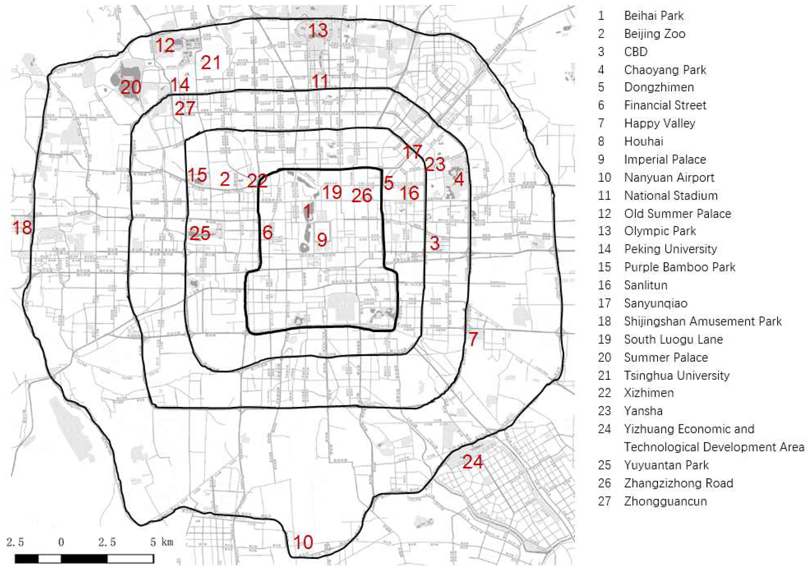
The GPS traces of 33,000 taxicabs in Beijing from 1 May 2015–31 July 2015 were collected. These data were the complete data set of an anonymous taxi company in Beijing during that period. They recorded traces of almost 50% of the taxis in service in Beijing, covering the whole study area. The status of a taxicab was sampled every minute for 24 h a day, including ID, position, timestamp, and whether a taxicab was occupied by passengers or not. The taxi traces were first cleaned by removing invalid or floating points. A sequence of consecutive points with an occupied status was identified as a passenger trip. Invalid trips that were less than 100 m or more than 100 km were filtered out. Then, the O-D pairs and their timestamps of each passenger trip were extracted. The pick-up point (O point) and drop-off point (D point) of each taxi trip were geo-coded to the grids. Any trip which had a point outside the study area was removed. All pick-ups and drop-offs were averaged on a daily basis and were allocated into 24 h accordingly. Finally, 15,033,149 passenger O-D trips were obtained. The spatial and temporal distributions of average pick-ups and drop-offs per day are shown in Figure 1. The temporal distributions are different during weekdays and weekends. From inside to outside of the map in Figure 1a, the ring roads are from the Second Ring Road to the Fifth Ring Road, in order. The locations of the place names that will be mentioned in the following sections are mapped in Appendix B.

4.2. Modeling

The spatiotemporal distribution differs not only between pick-ups and drop-offs, but also between weekdays and weekends. Therefore, STC-NMF should model passenger departures and arrivals on weekdays and weekends.
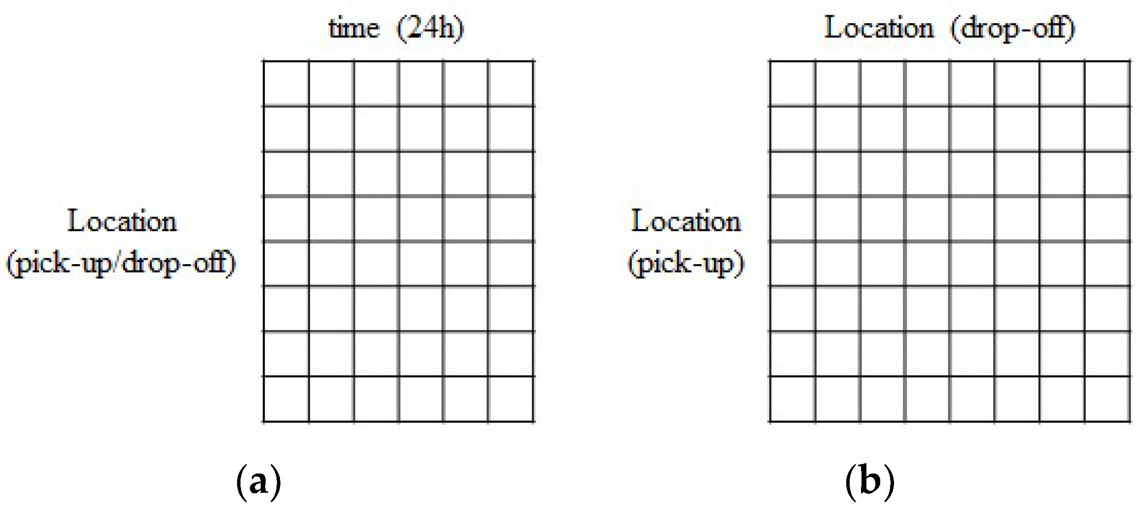
For the spatiotemporal pattern of departures, a location–time matrix was constructed (Figure 2a), in which a row denotes a location identified by a grid cell, a column denotes a time slot of 24 h a day, and an entry is the number of pick-ups in the location at the time. As a result, departures during weekdays and weekends were represented by two 900 × 24 matrices. Arrivals during weekdays and weekends were modeled by two location–time matrices of drop-offs in the same way. The objective function of the STC-NMF model for these location–time matrices is as Equation (8).
For the spatial interaction pattern, an O-D matrix was constructed (Figure 2b), in which both a row and a column denote locations, which are identified by grid cells, and an entry is the trip flows from the row location to the column location. For weekdays and weekends, two 900 × 900 location-location matrices were constructed. Spatial autocorrelations exist in both rows and columns, while temporal autocorrelations are ignored. Its objective function of the STC-NMF model is as Equation (9).
In the models, the parameters λ u , λ v , λ c , and λ r could be set as 0.1, after trial and error for the trade-off. The residual sum of squares (RSS)-based method [45] was employed to predetermine the optimal k because it is simple and easy to compute. After trying different k s, the k value at the inflection point of the RSS curve was determined as the optimal one.

4.3. Discovering Spatiotemporal Mobility Patterns

A taxi trip includes a pick-up point and a drop-off point, which represent a passenger’s departure and arrival, respectively. In a location, the frequency of departures represents the travel demand and the frequency of arrivals indicates the travel purpose. To discover intra-urban mobility patterns, four 900 × 24 location–time matrices were constructed for the STC-NMF model, i.e., matrices of pick-ups and drop-offs during weekdays and weekends. The RSSs of the factorized results of the four matrices exhibit that 4 was the optimal k value for the two pick-up matrices and 3 was optimal for the two drop-off matrices. Each matrix was factorized by the proposed STC-NMF model with the optimal k . As a result, k mobility patterns were discovered in the final U and V . U is the location–pattern matrix in which each column is a vector with a length of 900. The j th ( j k ) column of U represents the spatial distribution of the intensity of pattern # j over all grid cells, and the i th ( i 900 ) row of U is the contribution of each pattern in the i th cell. The pattern with the largest contribution in a cell is considered as the dominant mobility pattern at that location. V is the pattern–time matrix in which each row is a vector with a length of 24. The i th ( i k ) row of V represents temporal variations in the intensity of pattern # i in 24 h and the j th ( i 24 ) column of V is the contribution of each pattern in the j th time slot.

4.3.1. Mobility Patterns During Weekdays

Departure Patterns During Weekdays

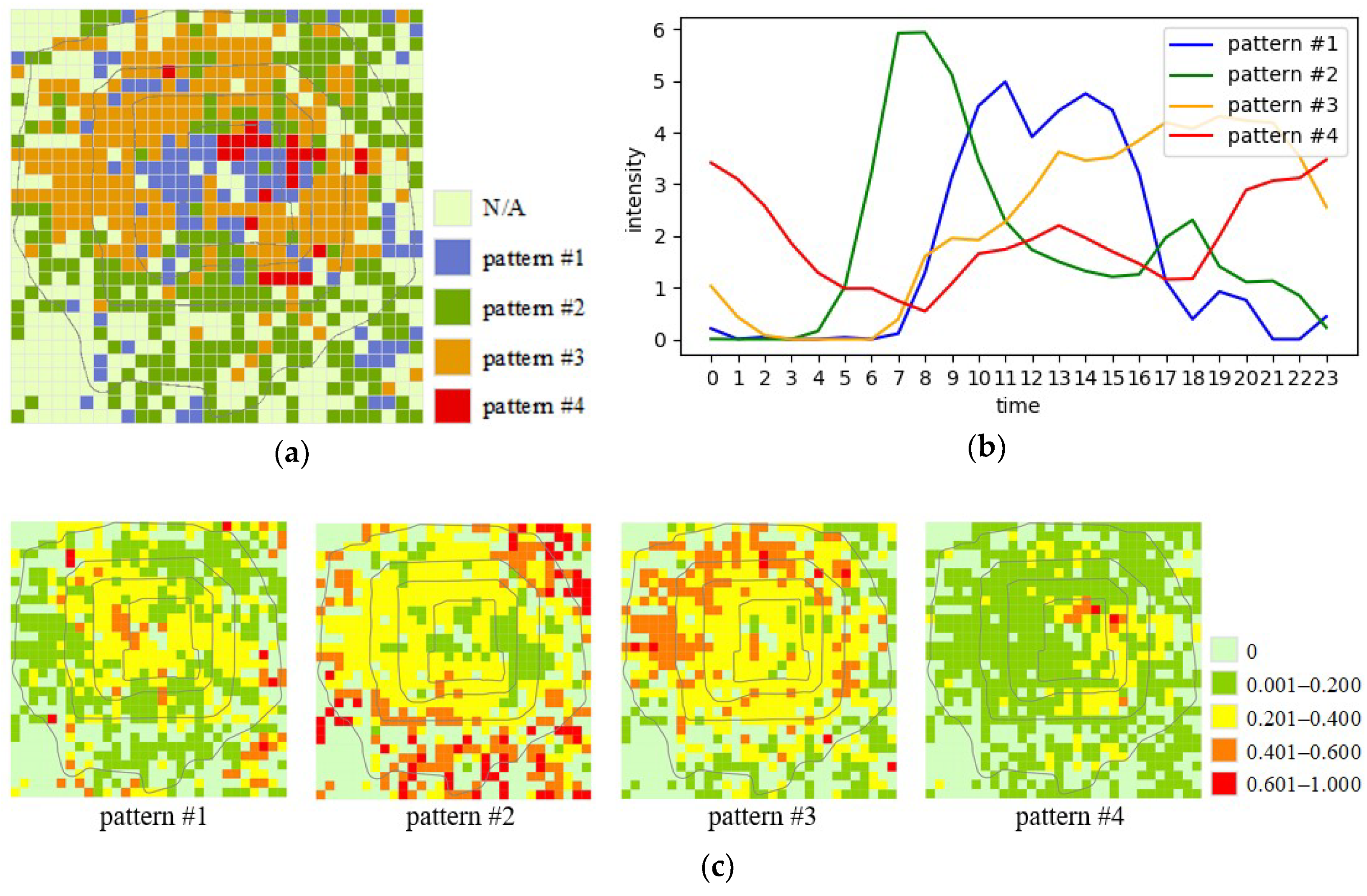
As mentioned previously, the optimal k was 4 for departures during weekdays, so four patterns were discovered (Figure 3). Figure 3a represents the dominant pattern in each grid cell. The dominant pattern was set as N/A for a cell if few pick-ups were observed, because no pattern can be recognized. Figure 3b plots the temporal variations of the four patterns in V . The x-axis in this figure denotes the time slots of 24 h and the y-axis is the pattern intensity that represents the relative departure frequencies. Figure 3c illustrates the spatial distributions of each pattern in U , in which the colors represent the normalized pattern intensity in locations.
In pattern #1, the grid cells with the highest intensity of departures are the places where business or high-tech districts were located, such as Zhongguancun in the northwest, the Yizhuang Economic and Technological Development Area in the southeast, and the Financial Street in the center. The temporal variation of this pattern peaked from 10:00 to 16:00, with a slight decline during lunchtime. Accordingly, pattern #1 is recognized as travel behavior to work, with business purposes.
Pattern #2 showed departures distributed mainly in the city peripheries, especially outside the Fourth Ring Road, where residential neighborhoods are clustered, as well as some office buildings. On the contrary, the high value of this pattern was rarely distributed in the city center within the Second Ring Road. The first peak time of this pattern was from 06:00 to 10:00, and the second peak was around 18:00. This pattern is believed to represent the travel behavior of commuting to work. Most people live in the peripheries of the urban area, where the rent is lower. Their commuting to work in the early morning results in the first travel peak. Moreover, the peak is sharp because people rush to work. The commuting from work to home is dispersive and not significant. Some nearby companies generated a small departure peak after work.
Pattern #3 is prominent in the west and north of the urban area in Beijing. Most of the intensive areas are large parks, such as Olympic Park in the north, Summer Palace in the northwest, Shijingshan Amusement Park in the west, and Chaoyang Park and Happy Valley in the east. The intensive travels were throughout the daytime, rising slowly from 08:00 to 22:00. This pattern can be considered the travel behavior for non-working purposes, especially for leisure.
Pattern #4 is unique in two aspects. First, the intensive departures were distributed only in two small areas. One is along Houhai, South Luogu Lane, and Zhangzizhong Road, another is around Sanlitun. Both areas are famous for bars and nightclubs. Second, most trips were generated at night, which is different from all the other three patterns, and the peak was from 00:00 to 01:00. As a result, this pattern is identified as the travel behavior for late night entertainments.
Overall, the four patterns account for 10.6%, 28.3%, 26.9%, and 2.6% of all grid cells, respectively, and the remaining 31.6% is N/A. Commuting and leisure-related travel were the main taxi trip purposes during weekdays, followed by work-related travel. Most taxi passengers departed to work from peripheral residences in the morning rush hours, traveled on business purposes in city centers during work time, got out by parks in the afternoon through the evening, and left bars in the late night.

Arrival Patterns During Weekdays

With an optimal k of 3, three patterns of arrivals during weekdays were discovered from drop-offs, represented in Figure 4. Figure 4a represents the dominant pattern in each grid cell. The value is N/A if no pattern is recognized, because the number of drop-offs was too few. The three patterns account for 30.2%, 10.9%, and 32.8% of this area, respectively. Pattern #1 and #3 are more dominant. Figure 4b,c illustrate the temporal variations and spatial distributions, respectively, of the three patterns.
Arrival pattern #1 is similar to departure pattern #1 during weekdays. Most drop-offs were distributed in the region with intensive office buildings within the Third Ring Road, and the high frequency times were from 09:00 to 17:00, with a slight decline during lunchtime (see Figure 4b). This pattern is recognized as arrivals due to business purposes during work time. Furthermore, it can be speculated that arrival pattern #1 is highly correlated with departure pattern #1 during weekdays, and the two mobility behaviors together make up complete journeys.
Arrival pattern #2 is also related to departure pattern #2 during weekdays. The high frequency drop-offs happened at 09:00 and 18:00, outside the Fourth Ring Road (see Figure 4b,c). This pattern is identified as the commuting pattern, in which the arrivals correspond to the departures of pattern #2 during weekdays.
Arrival pattern #3 during weekdays was mainly distributed around parks and other leisure places. The number of drop-offs increased significantly from 13:00, and peaked from 19:00 to 22:00. This pattern represents people’s arrivals, which are generated by the departures of pattern #3 during weekdays. The mobility of these two patterns is jointly caused by short-distance recreational travels.
Obviously, during weekdays, departure and arrival patterns are one-on-one correspondence. The corresponding pairs construct complete flows, which are categorized into business mobility flows, commuting flows, and leisure mobility flows. No significant arrival pattern was recognized which was related to departure pattern #4 for late night entertainment. People might leave bars intensively at late night, but their destinations are dispersed. On the other hand, people usually go to these entertainment places in scattered times. As a result, no intensive region or time of such drop-offs was detected.

4.3.2. Mobility Patterns During Weekends

Departure Patterns During Weekends

Departures at weekends were also decomposed into four mobility patterns, with the optimal k = 4 (Figure 5). The four patterns account for 29.0%, 0.7%, 4.5%, and 32.7% of this area, and the remaining 33.1% is N/A. Different from the travel patterns during weekdays, departures during weekends are mainly for leisure and entertainment purposes.
The departures of pattern #1 were mainly clustered in some famous tourist attractions, including the Imperial Palace, Beihai Park, Summer Palace, and Happy Valley. Temporally, it peaked in the afternoon. Therefore, this pattern is recognized as the departures after visiting a scenic spot. Pattern #2 during weekends is similar to pattern #4 during weekdays. The intensive mobility was around South Luogu Lane and Sanlitun at night. It was triggered by leaving entertainment venues late at night on weekends. The mobility of pattern #3 was distributed quite evenly, with a few high- or low-value regions. The intensity of most locations was 20–40%. Temporally, the mobility increased at sunset and peaked at 21:00. Thus, it is considered as normal behavior of taking taxis in the evening without typical purposes. The intensive areas of pattern #4 were mainly outside the Fourth Ring Road in the morning. It is considered as travels from personal residences to the city center, for various weekend activity purposes. As shown in Figure 5a, patterns #1 and #4 were more dominant than the other two, covering most areas of the city. It is popular for most people taking taxis to go out for weekend activities in the morning and return home in the afternoon.
By comparing Figure 3a and Figure 5a and comparing Figure 3b and Figure 5b, it was found that travel patterns of taxi passengers are different during weekdays and weekends, with respect to space and time. The variations during the weekend are more gradual than those during weekdays. Each pattern during weekends had only one peak, and those peaks did not have large overlaps. Given that people go out more arbitrarily during weekends, as a result, the travel volumes were relatively even in the four distinct periods of morning, afternoon, evening, and night, which are divided by three mealtimes.

Arrival Patterns During Weekends

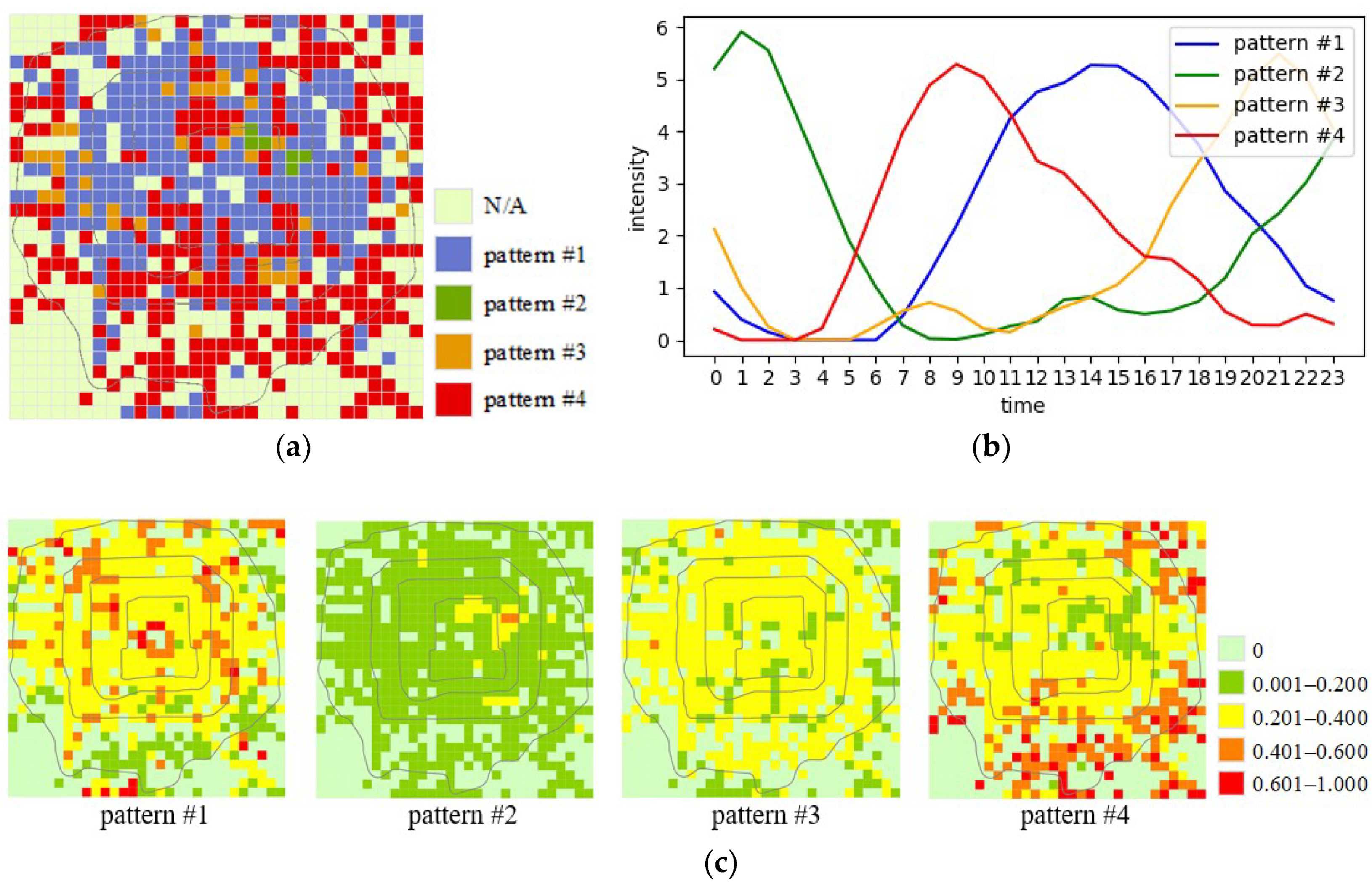
Similarly, three patterns were also found for arrivals during weekends (Figure 6), with the optimal k = 3 . Patterns #2 and #3 covered most areas (Figure 6a), with ratios of 33.8% and 37.3%, and pattern #1 only accounted for 0.2%. Figure 6b,c represent the temporal variations and the spatial distributions of the three patterns.
Pattern #1 is very special because its temporal curve has only one sharp peak, from 06:00 to 07:00. The peak indicates that some people arrived at their destination very early during weekends. The drop-offs were distributed sparsely, with relatively small quantities. Five regions with relatively high intensities can be recognized, which are represented as orange cells in pattern #1 of Figure 6c. The one orange cell in the northeast and the two in the southwest are where driving schools are located. Some people get there early on weekends to take a driving class. The orange area in the south is Nanyuan Airport, where some people catch early flights. The last one in the southeast is the Yizhuang Economic and Technological Development Area. Employees might go there in the morning to work overtime. In summary, pattern #1 is some people arriving at certain places for specific reasons on weekend mornings.
Pattern #2 is distributed dispersedly, with different intensities mixed together, in which the highest intensities were mostly outside the Third Ring Road. Its temporal curve is similar to the superposition of departure curves of pattern #2 and #3 during weekends. The arrival mobility continued from the afternoon through the late night. This pattern is estimated as the mobility of people returning home after weekend entertainment activities.
Pattern #3 is also dispersive in the city. Different from pattern #2, however, dense drop-offs covered almost all regions within the Third Ring Road. Most of the intensive areas are famous tourist attractions, especially around the Imperial Palace in the city center. The temporal curve peaks from 09:00 to 16:00. Therefore, this pattern shows arrivals at tourist attractions during the daytime. It is the combined result of departure patterns #1 and #4 during weekends.

4.4. Spatial Interaction Patterns

The pair of a pick-up and a drop-off is essential to construct a complete taxi trip. The movement of a passenger from the pick-up location to the drop-off location indicates the spatial interaction between the two places. Two 900 × 900 location–location matrices were constructed from the taxi O-D relationships of weekdays and weekends. The two matrices were factorized by the STC-NMF model to discover the spatial interaction patterns. The RSSs of the factorized results exhibit that the optimal k value was 8 for both matrices. Therefore, eight spatial interaction patterns were discovered from the final U and V of each O-D matrix. In the results, U T , which is the transpose of U , is the pattern–departure matrix, in which each row is a 900-length vector representing the departure contribution of the corresponding pattern in each location. V is the pattern–arrival matrix of the same size, in which each row represents the arrival contribution of each pattern in all locations. Both U T and V were normalized by rows to highlight the relative intensity differences of a pattern at different locations.
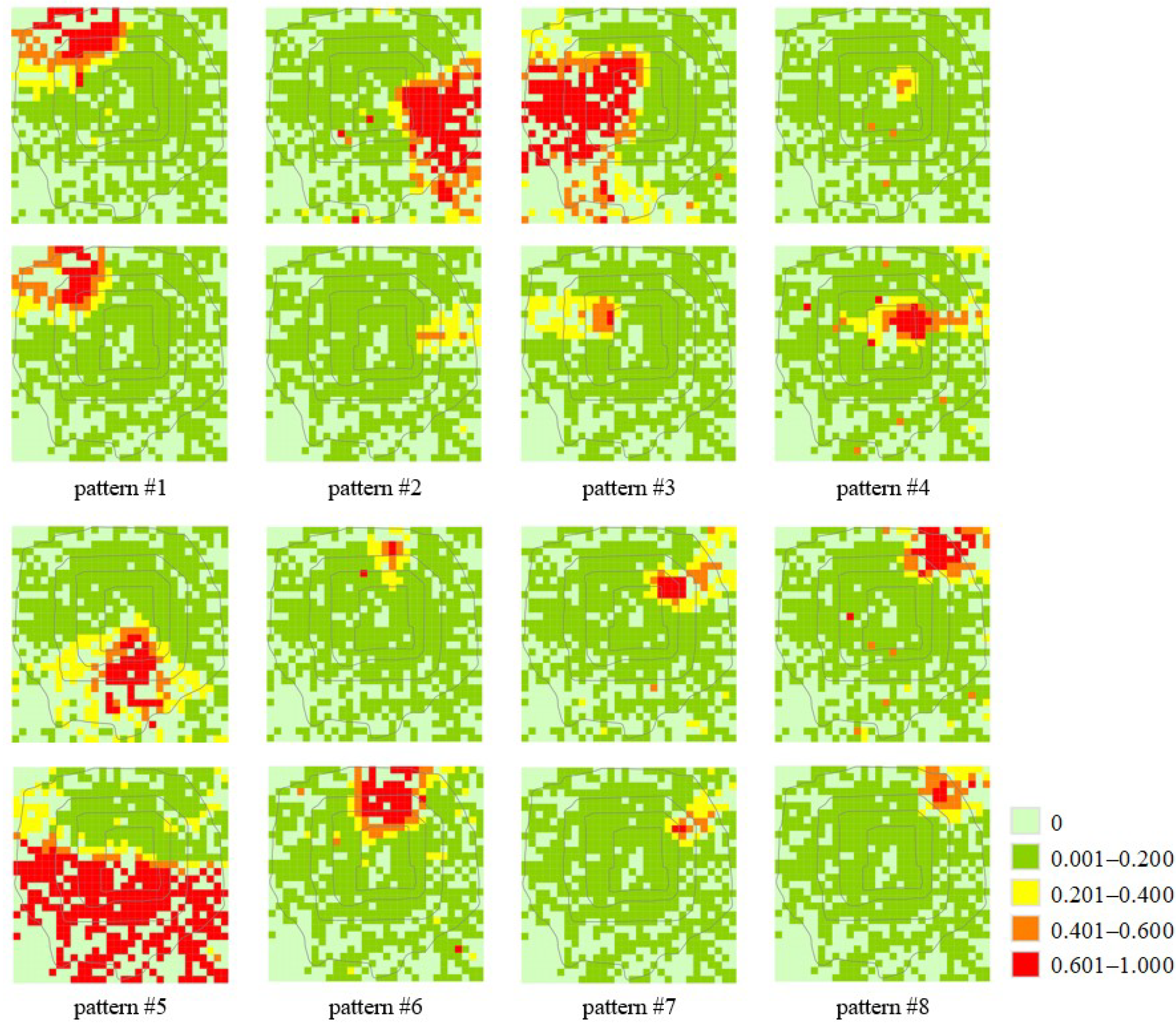
As a result, eight patterns of spatial interactions during weekdays were extracted, as shown in Figure 7. Each pair of maps is a spatial interaction pattern in terms of pick-ups and drop-offs, in which the above map is the departure distribution in U T and the below one is the corresponding arrival distribution in V . The colors in each map denote the normalized intensities of the corresponding pattern in U or V , which represent the relative frequency of travel flows. The eight interaction patterns reveal the taxi passengers’ mobility in different regions in Beijing. Through visualization, the dominant travel purpose in each interaction pattern can be identified by its consistency with the departure and arrival patterns in Figure 3, Figure 4, Figure 5 and Figure 6. This is considered to be the corresponding dominant departure or arrival trip purpose in the same grid cell. Pattern #1 was mainly located in the northwest of the city, which is a mixture of tour and work destinations. Pattern #2 was distributed in the east region, with dispersive intensive departures and small-scale arrivals. It is consistent with commuting travels from the east to the CBD (central business district). In pattern #3, the departures map shows high intensities in the west part of the city, which is mostly for leisure purposes. Some of the arrivals were around Xizhimen area, where a big subway interchange station and a railway station are located, and other intensive arrival regions, including Beijing Zoo and Purple Bamboo Park. Therefore, this pattern shows leisure travel to transportation hubs or famous parks in the west. Pattern #4 shows travel for business purpose from Dongzhimen, which is another transportation hub, to the nearby office locations. Pattern #5 shows mainly the commuting flows from work to home in the southern areas. Pattern #6 shows the leisure travel in the north, mainly from the National Stadium. Trips in pattern #7 are for business purposes, from around Dongzhimen and Sanyunqiao, both of which are transportation hubs, to the Yansha business districts. Pattern #8 consists of commuting flows in the northeast of the city. The eight interaction patterns exhibit different movement modes. In patterns #1, #7, and #8, departures were distributed similarly to arrivals. The dispersion of departures converged to concentrated arrival locations in patterns #2 and #3, which reveals the passenger-generating regions of the hubs or centers. Passengers were dispersed widely from centers in pattern #4, #5, and #6, which demonstrates the travel destinations from the centers.
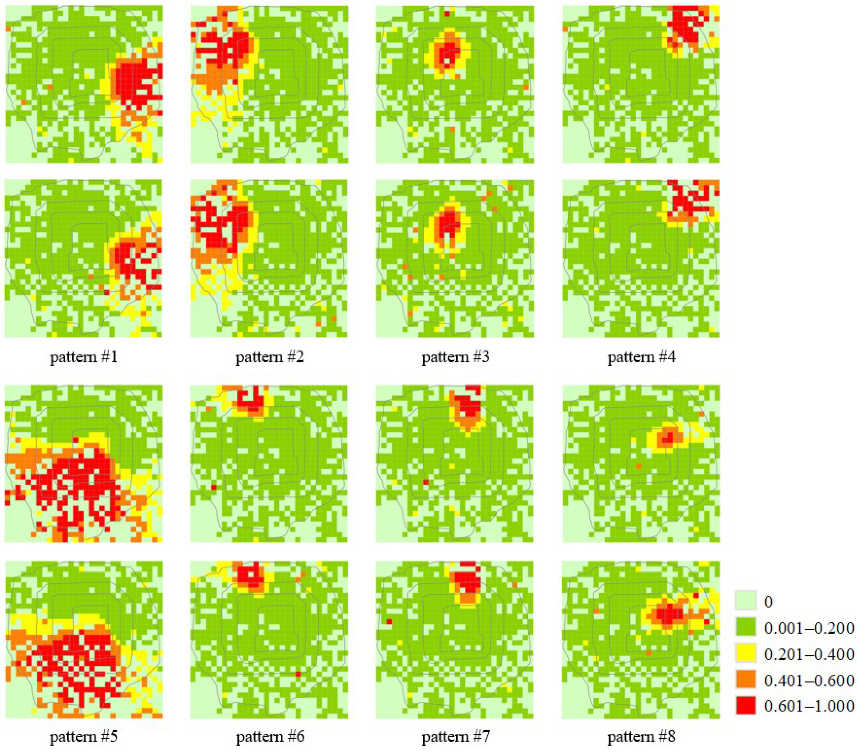
In the same way, the spatial interaction patterns during weekends are visualized in Figure 8. Each pair of maps is a spatial interaction pattern, in which the above map is the departure distribution and the bottom map is the corresponding arrival distribution. The interaction patterns have a certain consistency with the mobility patterns in Figure 3, Figure 4, Figure 5 and Figure 6, too. Because leisure travel dominated mobility during weekends, most interaction flows were for leisure purposes in different regions in the city, including around Chaoyang Park in the east (pattern #1), the Summer Palace and Old Summer Palace in the northwest (pattern #2), Beijing Zoo and Yuyuantan Park in the city center (pattern #3), and the National Stadium and the Olympic Park in the north (pattern #7). Some trips for shopping and entertainment were distributed around Zhongguancun, Peking University, and Tsinghua University in the north (pattern #6), and in Sanlitun and the CBD in the east (pattern #8). Patterns #4 and #5 show normal weekend activities without a distinct purpose. The former was concentrated in the residential areas of the northeast, and the latter was travels between private residences and the city center in large southwest regions. In all patterns, the departures were distributed similarly to arrivals, which means that dominant mobility flows are generated in local regions.
Both departures and arrivals in each spatial interaction pattern were significantly clustered. In each pattern, moreover, the intensive regions of the departure and the arrival overlapped very much. It indicates that the drop-off locations were usually near the pick-up locations in the same interactions. Of all the taxi trips, 84% were no more than 10 km, i.e., 10-cell length in the grid. As a result, the departure and arrival locations were spatially dependent, with a trend of short trips. Spatial interactions were more significant between near locations.
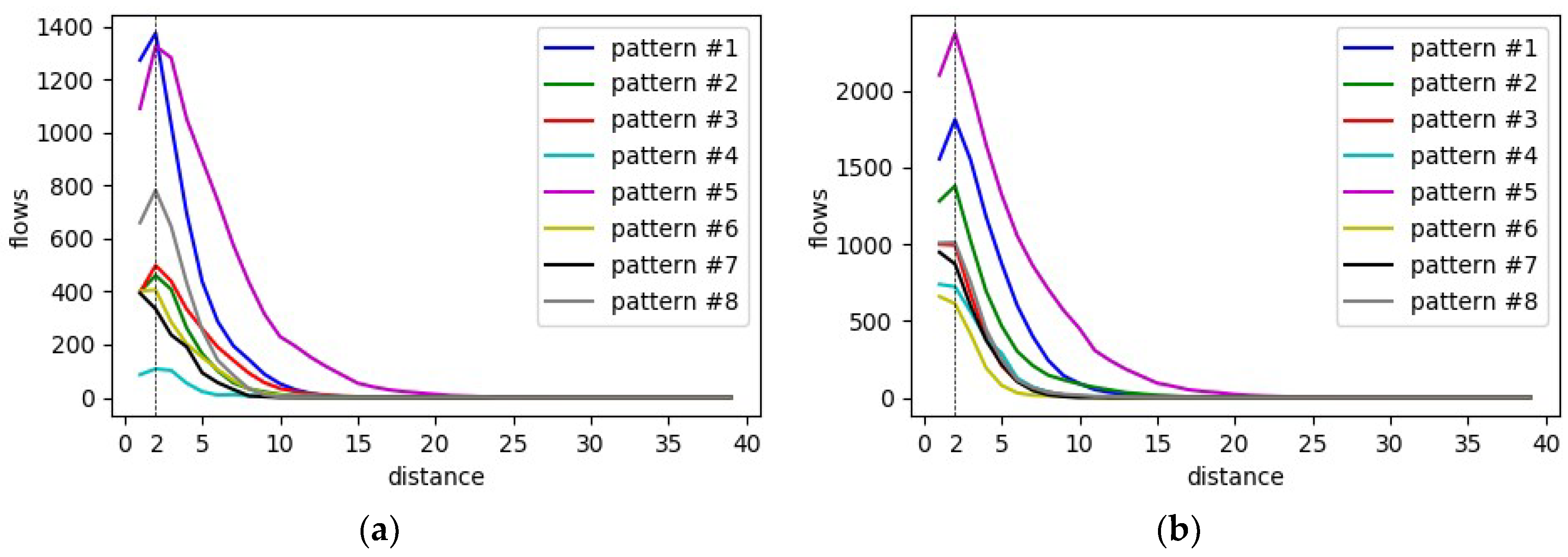
To illustrate such a tendency of short taxi travels in spatial interaction patterns, trips between the high-valued regions with relative intensity greater than 40% were extracted. These trips were the major flows of the corresponding pattern, because they occupied almost more than 35% of trips, but less than 10% of departure or arrival regions. The distance distribution of average major flow numbers per day during weekdays and weekends are plotted, respectively, in Figure 9. The distances are measured by cells. Major flows in each pattern exhibit a significant distance decay effect, and short taxi trips are preferred. The distance distributions of major flows follow the similar trends of the results generated from taxi trips in Shanghai, China by Liu et al. [8]. The main difference to Liu et al. [8] is that the major flows at a one-cell distance, i.e., less than 2 km, were relatively more. In such a distance, spatial interactions occur within the same cell or between neighbor cells. Then, the number reaches a peak at the two-cell distance, which is 2–4 km, which indicates that short-distance interactions are dominant. Subsequently, flows decline persistently with the increase in distance. All distribution curves followed a similar trend, with few intersections with each other. The spatial interactions of different patterns followed a similar distance decay effect. The difference is just the quantity.
It can also be noticed that the number of major flows during weekdays was much less than those on weekends. The purposes for which people take taxis during workdays are more diverse, so the origins, destinations, and then major flows are more spatially dispersed. On the contrary, taxi trips on weekends are mainly for leisure and entertainment, and the major flows are more clustered. The ratios of intensive grid cells in which the intensity of each interaction pattern and major flows were more than 40% are listed in Table 1. The ratio of intensive grid cells of a departure pattern was much different to that of the corresponding arrival pattern during workdays, while the difference was small on weekends. Taxi travels were much more dispersed during workdays. Meanwhile, the intensive grid cells occupied by complete major flows were less during workdays than on weekends. More diverse taxi trip purposes lead to more spatially dispersed mobility, then result in less major flows.
These discovered mobility and interaction patterns are the results of the types of taxi passengers, especially of their travel purposes. On the other hand, these patterns can also reveal travel purposes by supplementing other information. Some research has been conducted to recognize trip purposes from taxi trajectories, and main trip purposes were distinguished, including work-related, transportation transfer, dining, shopping, recreation, and schooling [20,47,48,49]. Each pattern of departures, arrivals, and spatial interactions discovered by STC-NMF was also related to some specific trip purposes. A better understanding of the spatiotemporal distribution of peoples’ travel purposes will contribute to sustainable transport and urban planning.

4.5. Verification

The proposed STC-NMF model was verified by being compared to classical NMF. No ground truth can validate the results directly. Clustering methods were employed by Cai et al. [50] and Chen et al. [51] to evaluate their NMF methods, and performed well. They demonstrated that the ability of NFM methods to provide perceptually reasonable feature representations can benefit clustering. Therefore, clustering was also utilized to compare the factorized results of STC-NMF and classical NMF. If a model factorizes a matrix more perfectly, the factorized features will be more distinct and more separated, and then the clustering result will be finer. The cluster results were then evaluated by the silhouette coefficient [52] to examine whether the patterns were recognized properly. For each item i in the cluster C i , its silhouette value was defined as:
s ( i ) = { b ( i ) a ( i ) max { a ( i ) , b ( i ) } if   | C i | > 1 0 if   | C i | = 1 ,
in which a ( i ) = 1 | C i | 1 j C i , j i d ( i , j ) measures the dissimilarity between i and all other items in the same cluster, b ( i ) = min k i 1 | C k | j C k d ( i , j ) measures the smallest mean dissimilarity of i to all items in any other cluster, and d ( i , j ) is the difference between the values of item i and j . Then, the silhouette coefficient of the clustering result is the mean s ( i ) over all data of the entire dataset. A larger silhouette coefficient indicates a better clustering result. The number of clusters that leads to the largest silhouette coefficient is the optimal one.
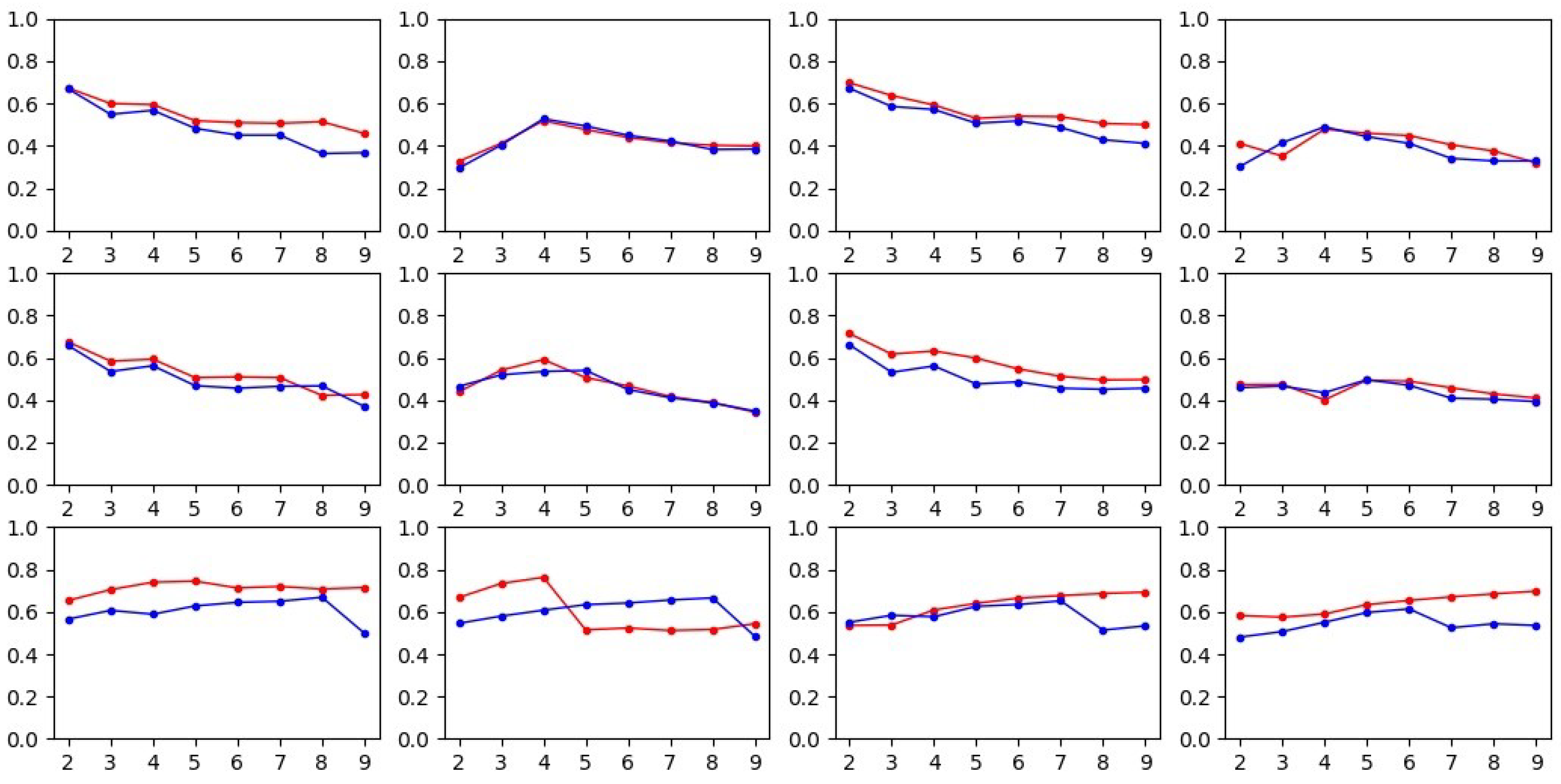
The twelve matrices that were constructed in Section 4.2 were factorized by STC-NMF and the classical NMF. In each result, the locations and time slots were clustered based on the factorized patterns by the k -medoids method, through setting a cluster number from 2 to 9. k -medoids [53] is a popular clustering method due to its simplicity and robustness to noise. The objective of its algorithm is to minimize the dissimilarity between items of a cluster and an item designated as the center (medoid) of that cluster under a given cluster number. The silhouette coefficients of all factorized results at every cluster number were compared in pairs, as shown in Figure 10, in which the results of STC-NMF are represented by red lines and the classical NMF by blue lines. The silhouette coefficients of the results factorized by the STC-NMF model are mostly larger than those of the classical NMF. In every result, moreover, the maximal silhouette coefficient of the STC-NMF model is always larger than that of the classical model. As a result, it can be believed that the STC-NMF model outperforms the classical model.

5. Conclusions

Rich human spatiotemporal mobility patterns in a city are embedded in taxi trajectories. By abstracting taxi trips as O-D pairs, travel flows can be represented by a matrix model. Although NMF is an optimal method to find latent patterns in the matrix, the accuracy of the results might be biased or distorted by its failure to deal with the spatial–temporal dependencies presented in taxi trips. By incorporating the spatiotemporal constraint into the classical model, the STC-NMF model was proposed. This novel method not only has the advantages of NMF to extract low-ranked latent factors, but also models spatial and temporal dependencies, and thus enhances pattern discovery under the constraint. It is superior to classical NMF methods when dealing with spatiotemporal data. The STC-NMF model is more consistent with the natural distribution of human mobility, therefore inherent spatial and temporal patterns embedded in taxi trajectories can be revealed. From passenger mobility during weekdays and weekends, four departure patterns and three arrival patterns were discovered from the location–time matrices, and eight spatial interaction patterns were found in the O-D matrix. Travel flows were distinctly different during working, commuting, and leisure hours during weekdays, while travel patterns were naturally distinguished by three mealtimes during weekends. Within certain time periods, intensive mobility was significantly recognized in particular regions, which can be related to the land uses in those areas. The interaction flows between locations exhibited a significant distance decay tendency, and short taxi trips were preferred. The patterns obtained by STC-NMF give low-ranked representations of massive taxi trips. The primary latent features are revealed distinctly. After incorporating spatial and temporal dependencies in this model, bias and distortion in the results were reduced. The novel model and discovered patterns are useful for predicting taxi demands, understanding intra-urban mobility patterns, and enhancing sustainable urban transportations. The proposed model is also generally applicable for other spatiotemporal interactions, beyond taxi trips.
More effort is needed to improve the STC-NMF model. For example, more different matrix representations for taxi trajectories can be investigated to discover other meaningful mobility patterns. Moreover, tensor factorization, as an extension of matrix factorization, is capable of decomposing higher dimensional datasets. This will be promising for embedding spatiotemporal dependencies into tensor factorization methods for mining human mobility in multiple dimensions. At the current stage, however, it will be a challenge to solve a spatiotemporal constraint tensor factorization model due to its complexity.

Author Contributions

Conceptualization, Y.G., J.L. and Y.L.; methodology, Y.G. and J.L; formal analysis, J.L. and Y.G; writing—original draft preparation, Y.G., J.L. and Y.X; writing—review and editing, L.M.; supervision, Y.L.; Funding Acquisition, Y.L.

Funding

This research was funded by the National Key Research and Development Program of China, grant number 2017YFB0503602; and the National Natural Science Foundation of China, grant number 41625003.

Conflicts of Interest

The authors declare no conflict of interest.

Appendix A

Frobenius norm can be defined as the square root of the sum of all elements [54], i.e.,
R F = i m j n R i j 2 .
It is also equal to the square root of the matrix trace of R R T , so,
R F = t r ( R R T ) ,
where t r ( · ) refers to the matrix trace function. Through the Frobenius norm expansion of Equation (A2), the objective function in Equation (7) is transformed to:
f ( U , V ) = t r [ ( R U V ) ( R U V ) T ] + λ u t r [ U T U ] + λ v t r [ V T V ]     + λ r h n i m j m W i j r ( R i h R j h ) 2 + λ c h m i n j n W i j c ( R h i R h j ) 2 .
For the row autocorrelation term, let L r = D r + E r W r , where D r ,   E r + m × m , D i i r = 1 2 j m W i j r and E i i r = 1 2 j m W j i r , then,
1 2 h n i m j m W i j r ( R i h R j h ) 2 = t r [ R T L r R ] .
It can be observed that L r is definite if Wr is definite. The proof of Equation (A4) is as follows.
The right side can be written as:
= t r [ R T ( D r + E r W r ) R ] = t r [ R T D r R ] + t r [ R T E r R ] t r [ R T W r R ] = h n i m j m R h i T D i j r R j h + h n i m j m R h i T E i j r R j h h n i m j m R h i T W i j r R j h .
D r and E r are diagonal matrices, so the above equation can be rewritten as:
= h n i m R h i T D i i r R i h + h n i m R h i T E i i r R i h h n i m j m R h i T W i j r R j h       = h n i m D i i r R i h 2 + h n i m E i i r R i h 2 h n i m j m R i h W i j r R j h .
Let D i i r = 1 2 j m W i j r ,   E i i r = 1 2 j m W j i r , then the above equation can be represented as:
= 1 2 h n i m j m W i j r R i h 2 + 1 2 h n i m j m W j i r R i h 2 h n i m i m R i h W i j r R j h       = 1 2 h n i m j m W i j r ( R i h R j h ) 2 .
Thus, the Equation (A4) is proved.
In the same way, for the column autocorrelation term, it can be transformed as:
1 2 h m i n j n W i j c ( R h i R h j ) 2 = t r [ R T L c R ] ,
where L c = D c + E c W c , and D c , E c + n × n , D i i c = 1 2 j n W i j c , E i i c = 1 2 j n W j i c .
Finally, the objective function is expressed as:
f ( U , V ) = t r [ ( R U V ) ( R U V ) T ] + λ u t r [ U T U ] + λ v t r [ V T V ] + λ r t r [ R T L r R ] + λ c t r [ R L c R T ] .
To solve the STC-NMF model, according to the multiplicative update algorithm [41], f ( U , V ) / U and f ( U , V ) / V are solved first as:
f ( U , V ) U = [ t r ( R U V ) ( R U V ) T + λ u t r [ U T U ] + λ v t r [ V T V ] + λ r t r [ R T L r R ] + λ c t r [ R L c R T ] ] U        = 2 R V T + 2 U V V T + 2 λ u U + λ r ( L r T + L r ) U V V T + λ c U V ( L c + L c T ) V T , f ( U , V ) V = [ t r ( R U V ) ( R U V ) T + λ u t r [ U T U ] + λ v t r [ V T V ] + λ r t r [ R T L r R ] + λ c t r [ R L c R T ] ] V                = 2 U T R + 2 U T U V + 2 λ v V + λ r U T ( L r + L r T ) U V + λ c U T U V ( L c T + L c ) .
To guarantee the results in each iteration step to be non-negative, the iteration multiplier is obtained with the negative part of the partial derivatives as the numerator and the positive part as the denominator [55]. Then, the iteration formula is:
V i j V i j ( U T R ) i j [ U T U V + λ v V ( n 1 ) + λ r 2 U T ( L r + L r T ) U V + λ c 2 U T U V ( L c T + L c ) ] i j , U i j U i j ( R V T ) i j [ U V V T + λ u U ( n 1 ) + λ r 2 ( L r T + L r ) U V V T + λ c 2 U V ( L c + L c T ) V T ] i j .

Appendix B

The locations of the place names that are mentioned in the paper are mapped in Figure A1.
Figure A1. The locations of the place names.
Sustainability 11 04214 g0a1

References

  1. Bruun, E.; Givoni, M. Sustainable mobility: Six research routes to steer transport policy. Nature 2015, 523, 29–31. [Google Scholar] [CrossRef] [PubMed] [Green Version]
  2. Gillis, D.; Semanjski, I.; Lauwers, D. How to monitor sustainable mobility in cities? Literature review in the frame of creating a set of sustainable mobility indicators. Sustainability 2016, 8, 29. [Google Scholar] [CrossRef]
  3. Jung, J.; Jayakrishnan, R.; Choi, K. Dually sustainable urban mobility option: Shared-taxi operations with electric vehicles. Int. J. Sustain. Transp. 2017, 11, 567–581. [Google Scholar] [CrossRef]
  4. Li, M.; Dong, L.; Shen, Z.; Lang, W.; Ye, X. Examining the interaction of taxi and subway ridership for sustainable urbanization. Sustainability 2017, 9, 242. [Google Scholar] [CrossRef]
  5. Nikulina, V.; Simon, D.; Ny, H.; Baumann, H. Context-adapted urban planning for rapid transitioning of personal mobility towards sustainability: A systematic literature review. Sustainability 2019, 11, 1007. [Google Scholar] [CrossRef]
  6. Zheng, Y. Trajectory data mining: An overview. ACM Trans. Intell. Syst. Technol. 2015, 6, 1–41. [Google Scholar] [CrossRef]
  7. Jiang, B.; Yin, J.; Zhao, S. Characterizing the human mobility pattern in a large street network. Phys. Rev. E 2009, 80, 021136. [Google Scholar] [CrossRef] [Green Version]
  8. Liu, Y.; Kang, C.; Gao, S.; Xiao, Y.; Tian, Y. Understanding intra-urban trip patterns from taxi trajectory data. J. Geogr. Syst. 2012, 14, 463–483. [Google Scholar] [CrossRef]
  9. Li, B.; Zhang, D.; Sun, L.; Chen, C.; Li, S.; Qi, G.; Yang, Q. Hunting or waiting? Discovering passenger-finding strategies from a large-scale real-world taxi dataset. In Proceedings of the IEEE International Conference on Pervasive Computing and Communications (PERCOM), Seattle, WA, USA, 21–25 March 2011; pp. 63–68. [Google Scholar] [CrossRef]
  10. Yuan, N.J.; Zheng, Y.; Zhang, L.; Xie, X. T-Finder: A recommender system for finding passengers and vacant taxis. IEEE Trans. Knowl. Data Eng. 2013, 25, 2390–2403. [Google Scholar] [CrossRef]
  11. Kang, C.; Qin, K. Understanding operation behaviors of taxicabs in cities by matrix factorization. Comput. Environ. Urban Syst. 2016, 60, 79–88. [Google Scholar] [CrossRef]
  12. Gao, Y.; Jiang, D.; Xu, Y. Optimize taxi driving strategies based on reinforcement learning. Int. J. Geogr. Inf. Sci. 2018, 32, 1677–1696. [Google Scholar] [CrossRef]
  13. Castro, P.S.; Zhang, D.; Chen, C.; Li, S.; Pan, G. From taxi GPS traces to social and community dynamics: A survey. ACM Comput. Surv. 2013, 46, 17. [Google Scholar] [CrossRef]
  14. Liu, X.; Gong, L.; Gong, Y.; Liu, Y. Revealing travel patterns and city structure with taxi trip data. J. Transp. Geogr. 2015, 43, 78–90. [Google Scholar] [CrossRef] [Green Version]
  15. Zhu, X.; Guo, D. Urban event detection with big data of taxi OD trips: A time series decomposition approach. Trans. GIS 2017, 21, 560–574. [Google Scholar] [CrossRef]
  16. Hu, Y.; Miller, H.J.; Li, X. Detecting and analyzing mobility hotspots using surface networks. Trans. GIS 2014, 18, 911–935. [Google Scholar] [CrossRef]
  17. Guo, D.; Zhu, X.; Jin, H.; Gao, P.; Andris, C. Discovering spatial patterns in origin-destination mobility data. Trans. GIS 2012, 16, 411–429. [Google Scholar] [CrossRef]
  18. Peng, C.; Jin, X.; Wong, K.-C.; Shi, M.; Liò, P. Collective human mobility pattern from taxi trips in urban area. PLoS ONE 2012, 7, e34487. [Google Scholar] [CrossRef]
  19. Scholz, R.W.; Lu, Y. Detection of dynamic activity patterns at a collective level from large-volume trajectory data. Int. J. Geogr. Inf. Sci. 2014, 28, 946–963. [Google Scholar] [CrossRef]
  20. Gong, L.; Liu, X.; Wu, L.; Liu, L. Inferring trip purposes and uncovering travel patterns from taxi trajectory data. Cartogr. Geogr. Inf. Sci. 2015, 43, 103–114. [Google Scholar] [CrossRef]
  21. Wang, P.; Fu, Y.; Liu, G.; Hu, W.; Aggarwal, C. Human mobility synchronization and trip purpose detection with mixture of hawkes processes. In Proceedings of the KDD’17, Halifax, NS, Canada, 13–17 August 2017. [Google Scholar] [CrossRef]
  22. Zhan, X.; Ukkusuri, S.; Yang, C. A Bayesian mixture model for short-term average link travel time estimation using large-scale limited information trip-based data. Autom. Constr. 2016, 72, 237–246. [Google Scholar] [CrossRef] [Green Version]
  23. Zheng, Z.; Zhou, S. Scaling laws of spatial visitation frequency: Applications for trip frequency prediction. Comput. Environ. Urban Syst. 2017, 64, 332–343. [Google Scholar] [CrossRef]
  24. Liu, X.; Kang, C.; Gong, L.; Liu, Y. Incorporating spatial interaction patterns in classifying and understanding urban land use. Int. J. Geogr. Inf. Sci. 2016, 30, 334–350. [Google Scholar] [CrossRef]
  25. Zhang, W.; Qi, G.; Pan, G.; Lu, H.; Li, S.; Wu, Z. City-scale social event detection and evaluation with taxi traces. ACM Trans. Intell. Syst. Technol. 2015, 6, 40. [Google Scholar] [CrossRef]
  26. Lee, D.D.; Seung, H.S. Learning the parts of objects by non-negative matrix factorization. Nature 1999, 401, 788–791. [Google Scholar] [CrossRef] [PubMed]
  27. Berry, M.W.; Browne, M.; Langville, A.N.; Pauca, V.P.; Plemmons, R.J. Algorithms and Applications for Approximate Nonnegative Matrix Factorization. Comput. Stat. Data Anal. 2007, 52, 155–173. [Google Scholar] [CrossRef]
  28. Gillis, N. The why and how of nonnegative matrix factorization. In Regularization, Optimization, Kernels, and Support Vector Machines 2014; Suykens, J., Signoretto, M., Argyriou, A., Eds.; Chapman & Hall/CRC: Boca Raton, FL, USA, 2014; pp. 257–291. [Google Scholar]
  29. Guillamet, D.; Vitrià, J. Non-negative matrix factorization for face recognition. In Lecture Notes in Artificial Intelligence; Escrig, M.T., Toledo, F., Golobardes, E., Eds.; Springer: Berlin/Heidelberg, Germany, 2002; Volume 2504, pp. 336–344. [Google Scholar] [CrossRef]
  30. Arora, S.; Ge, R.; Halpern, Y.; Mimno, D.; Moitra, A.; Sontag, D.; Wu, Y.; Zhu, M. A Practical Algorithm for Topic Modeling with Provable Guarantees. In Proceedings of the 30th International Conference on Machine Learning, Atlanta, GA, USA, 16–21 June 2013; pp. 280–288. [Google Scholar]
  31. Bell, R.; Koren, Y.; Volinsky, C. Matrix factorization techniques for recommender systems. IEEE Comput. 2009, 42, 30–37. [Google Scholar] [CrossRef]
  32. Saito, S.; Hirata, Y.; Sasahara, K.; Suzuki, H. Tracking time evolution of collective attention clusters in twitter: Time evolving nonnegative matrix factorisation. PLoS ONE 2015, 10, e0139085. [Google Scholar] [CrossRef]
  33. Yong, N.; Ni, S.; Shen, S.; Chen, P.; Ji, X. Uncovering stable and occasional human mobility patterns: A case study of the Beijing subway. Phys. A Stat. Mech. Its Appl. 2018, 492, 28–38. [Google Scholar] [CrossRef]
  34. Cazabet, R.; Jensen, P.; Borgnat, P. Tracking the evolution of temporal patterns of usage in bicycle-Sharing systems using nonnegative matrix factorization on multiple sliding windows. Int. J. Urban Sci. 2018, 22, 147–161. [Google Scholar] [CrossRef]
  35. Graells-Garrido, E.; Caro, E.; Parra, D. Inferring modes of transportation using mobile phone data. EPJ Data Sci. 2018, 7, 49. [Google Scholar] [CrossRef]
  36. Maeda, T.N.; Shiode, N.; Zhong, C.; Mori, J.; Sakimoto, T. Detecting and understanding urban changes through decomposing the numbers of visitors’s arrivals using human mobility data. J. Big Data 2019, 6, 4. [Google Scholar] [CrossRef]
  37. Pang, J.; Huang, J.; Yang, X.; Wang, Z.; Yu, H.; Huang, Q.; Yin, B. Discovering fine-grained spatial pattern from taxi trips: Where point process meets matrix decomposition and factorization. IEEE Trans. Intell. Transp. Syst. 2018, 19, 3208–3219. [Google Scholar] [CrossRef]
  38. Zheng, V.W.; Zheng, Y.; Xie, X.; Yang, Q. Collaborative location and activity recommendations with GPS history data. In Proceedings of the 19th International Conference on World Wide Web, Raleigh, NC, USA, 26–30 April 2010; pp. 1029–1038. [Google Scholar] [CrossRef]
  39. Shang, J.; Zheng, Y.; Tong, W.; Chang, E.; Yu, Y. Inferring gas consumption and pollution emission of vehicles throughout a city. In Proceedings of the 20th ACM SIGKDD International Conference on Knowledge Discovery and Data Mining, New York, NY, USA, 24–27 August 2014; pp. 1027–1036. [Google Scholar] [CrossRef]
  40. Tobler, W.R. A computer movie simulating urban growth in the detroit region. Econ. Geogr. 1970, 46 (Suppl. 1), 234–240. [Google Scholar] [CrossRef]
  41. Lee, D.D.; Seung, H.S. Algorithms for non-negative matrix factorization. In Advances in Neural Information Processing Systems 13, Proceedings of the 2000 Conference, Denver, CO, USA, 27–30 November 2000; Leen, T.K., Dietterich, T.G., Tresp, V., Eds.; MIT Press: Cambridge, MA, USA, 2001; pp. 556–562. [Google Scholar]
  42. Ambroise, C.; Govaert, G. Convergence of an EM-type algorithm for spatial clustering. Pattern Recognit. Lett. 1998, 19, 919–927. [Google Scholar] [CrossRef]
  43. Liu, J.; Zhang, Y.; Li, Z.; Hu, L. Correlation consistency constrained probabilistic matrix factorization for social tag refinement. Neurocomputing 2013, 119, 3–9. [Google Scholar] [CrossRef]
  44. Brunet, J.P.; Tamayo, P.; Golub, T.R.; Mesirov, J.P. Metagenes and molecular pattern discovery using matrix factorization. Proc. Natl. Acad. Sci. USA 2004, 101, 4164–4169. [Google Scholar] [CrossRef] [Green Version]
  45. Hutchins, L.N.; Murphy, S.M.; Singh, P.; Graber, J.H. Position-dependent motif characterization using non-negative matrix factorization. Bioinformatics 2008, 24, 2684–2690. [Google Scholar] [CrossRef] [PubMed]
  46. Chen, Z.; Cichocki, A. Nonnegative Matrix Factorization with Temporal Smoothness and/or Spatial Decorrelation Constraints; RIKEN Brain Science Institute: Saitama, Japan, 2005; Volume 68. [Google Scholar]
  47. Chen, C.; Jiao, S.; Zhang, S.; Liu, W.; Feng, L.; Wang, Y. TripImputor: Real-time imputing taxi trip purpose leveraging multi-sourced urban data. IEEE Trans. Intell. Transp. Syst. 2018, 19, 3292–3304. [Google Scholar] [CrossRef]
  48. Meng, C.; Cui, Y.; He, Q.; Su, L.; Gao, J. Towards the inference of travel purpose with heterogeneous urban data. IEEE Trans. Big Data 2019. [Google Scholar] [CrossRef]
  49. Chen, C.; Liao, C.; Xie, X.; Wang, Y.; Zhao, J. Trip2Vec: A deep embedding approach for clustering and profiling taxi trip purposes. Pers. Ubiquitous Comput. 2019, 23, 53–66. [Google Scholar] [CrossRef]
  50. Cai, D.; He, X.; Han, J.; Huang, T.S. Graph regularized nonnegative matrix factorization for data representation. IEEE Trans. Pattern Anal. Mach. Intell. 2011, 33, 1548–1560. [Google Scholar] [CrossRef] [PubMed]
  51. Chen, X.; Li, C.; Liu, H.; Cai, D. Spatially correlated nonnegative matrix factorization. Neurocomputing 2014, 139, 15–21. [Google Scholar] [CrossRef]
  52. Rousseeuw, P.J. Silhouettes: A graphical aid to the interpretation and validation of cluster analysis. J. Comput. Appl. Math. 1987, 20, 53–65. [Google Scholar] [CrossRef] [Green Version]
  53. Rousseeuw, P.J.; Kaufman, L. Clustering by Means of Medoids. In Data Analysis Based on the L1-Norm and Related Methods; Dodge, Y., Ed.; North-Holland/Elsevier: Amsterdam, The Netherlands, 1987; pp. 405–416. [Google Scholar]
  54. Golub, G.H.; van Loan, C.F. Matrix Computations, 3rd ed.; The John Hopkins University Press: Baltimore, MD, USA, 1996; p. 55. [Google Scholar]
  55. Tjoa, S.K.; Liu, K.J.R. Multiplicative update rules for nonnegative matrix factorization with co-occurrence constraints. In Proceedings of the IEEE International Conference on Acoustics Speech and Signal Processing (ICASSP), Dallas, TX, USA, 14–19 March 2010; pp. 449–452. [Google Scholar] [CrossRef]
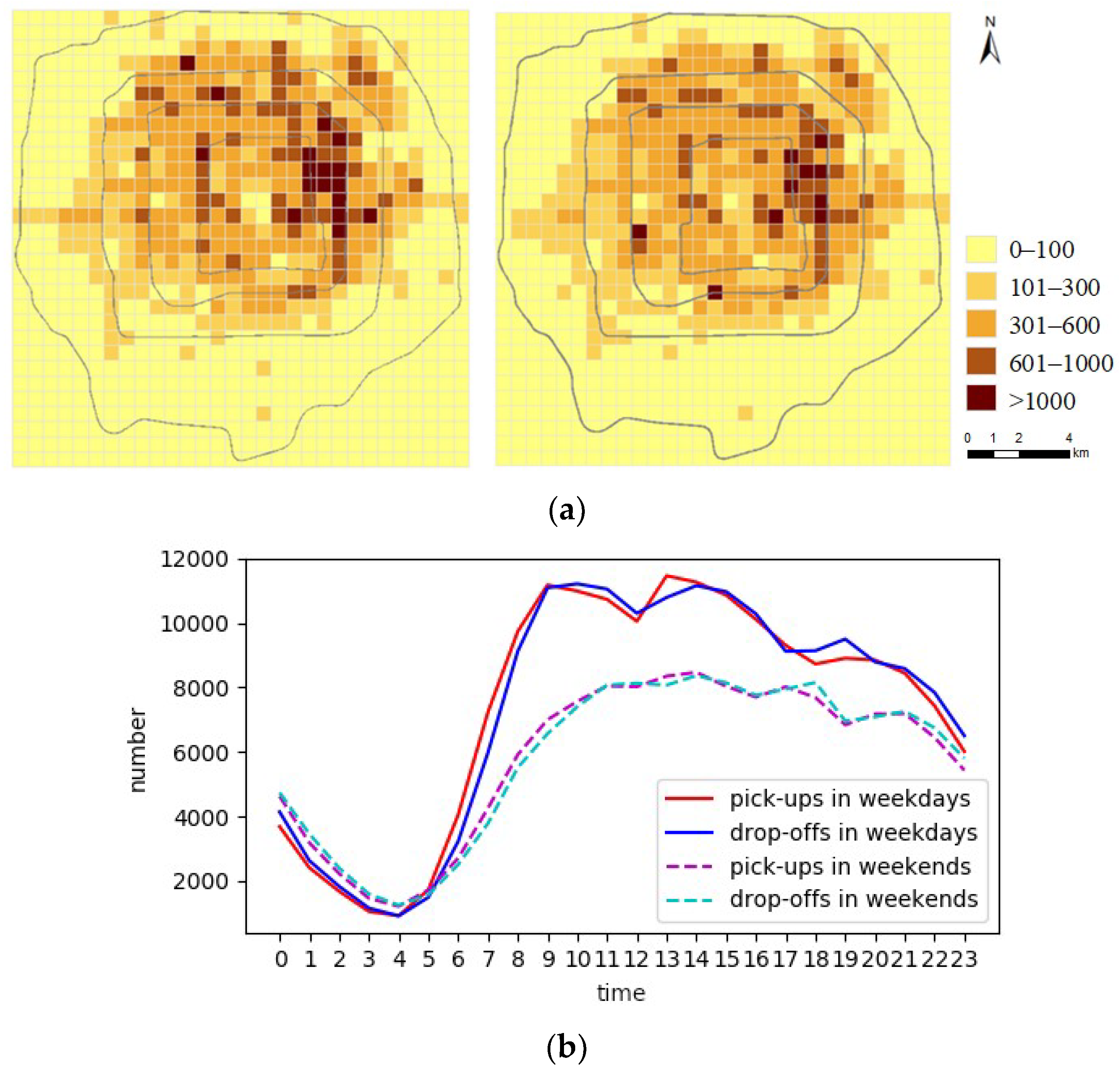
Figure 1. Distributions of origin and destination (O-D) pairs in Beijing. (a) Spatial distributions of average pick-ups (left) and drop-offs (right) per day. (b) Temporal distributions of average pick-ups and drop-offs during weekdays and weekends.
Sustainability 11 04214 g001
Figure 2. The constructed matrices. (a) A location–time matrix. (b) An O-D matrix.
Sustainability 11 04214 g002
Figure 3. Spatiotemporal patterns of departures during weekdays. (a) The spatial distribution of dominant patterns. (b) The temporal variations of the four patterns. (c) The spatial distribution of the four patterns.
Sustainability 11 04214 g003
Figure 4. Spatiotemporal patterns of arrivals during weekdays. (a) The spatial distribution of dominant patterns. (b) The temporal variations of the three patterns. (c) The spatial distribution of the three patterns.
Sustainability 11 04214 g004
Figure 5. Spatiotemporal patterns of departures during weekends. (a) The spatial distribution of dominant patterns. (b) The temporal variations of the four patterns. (c) The spatial distribution of the four patterns.
Sustainability 11 04214 g005
Figure 6. Spatiotemporal patterns of arrivals during weekends. (a) The spatial distribution of the dominant patterns. (b) The temporal variations of the three patterns. (c) The spatial distribution of the three patterns.
Sustainability 11 04214 g006
Figure 7. Spatial interaction patterns during weekdays.
Sustainability 11 04214 g007
Figure 8. Spatial interaction patterns during weekends.
Sustainability 11 04214 g008
Figure 9. Distance distributions of major flows per day during (a) weekdays and (b) weekends.
Sustainability 11 04214 g009
Figure 10. Silhouette coefficients of clustering patterns of STC-NMF (red) and classical NMF (blue). From left to right and top to bottom, the plots are the results of U of pick-ups during weekdays, V of pick-ups during weekdays, U of pick-ups during weekends, V of pick-ups during weekends, U of drop-offs during weekdays, V of drop-offs during weekdays, U of drop-offs during weekends, V of drop-offs during weekends, U of interactions during weekdays, V of interactions during weekdays, U of interactions during weekends, and V of interactions during weekends.
Sustainability 11 04214 g010
Table 1. Ratios of intensive grid cells (%).
PeriodMobilitySpatial Interaction Patterns
#1#2#3#4#5#6#7#8
workdaydeparture8.0015.3321.220.677.671.002.896.22
arrival6.780.561.565.2234.567.781.113.00
major flow5.560.561.440.336.561.000.443.00
weekenddeparture10.8911.443.565.4426.333.333.892.00
arrival8.2212.674.335.1123.563.443.674.67
major flow6.8910.003.004.0018.892.563.113.89