Abstract
One of the most important parameters in sustainable urban land valuation is the risk premium. Correct assessment of the risk premium is essential for sustainable valuation. Generally, it is estimated that traditional financial models or historic rates do not take into account the specific risk factors of an investment project. In this paper, we propose a sustainable model to obtain it. It is based on investment risk factors and the urban planning land development stages. We conducted a study in Badajoz, Spain, on four urban stages: first, land without an execution program; second, land with an execution program; third, land with reparceling; and fourth, fully developed and urbanized land. We calculated one different risk premium value for each urban stage. The results show that with this model, we can obtain the risk premium at any time during urban planning development. The urban stage is one of the most influential factors in the risk premium value. It decreases during urban planning development, and fully developed and urbanized land has a lower risk premium.
1. Introduction
Since the beginning of the 21st century, the concept of sustainable urban development (SUD) has been a popular topic due to its importance for the rational growth and sustainable development of cities [1,2,3]. SUD implies that relations between society and the surrounding environment are not catalysts to uncontrolled growth, but they do induce qualitative improvements that favor development over growth. This is the main difference between growth and development: There should be no indefinite growth, while there must indeed be continued development. Growth has to be kept to a minimum according to desired development in order not to compromise essential resources for future generations. SUD prioritizes the concept of urban regeneration over the idea of unlimited growth in such a fashion that when new developments are intended, they are justified. To ensure the effectiveness of SUD, its inspiring principles must be reflected in the urban planning instruments [3].
Land is a scarce, limited natural resource [4,5], and one of the main goals of urban and territorial planning instruments is finding good use for land itself, which must be done following sustainable guidelines. Amidst the process of urban planning, the establishment of land classification and edification intensity and their use imply the attribution of the economic value to the target soil of planning itself.
The aspects most directly associated with SUD are land and development. Given this fact, it is essential to establish an objective methodology for land valuation with efficient development in order to avoid speculation and to get the most sustainable value for land, also taking into account the assignment of development planning, excluding hard or impossible realization expectations. As development planning progresses, the land goes through different stages or urbanization levels, and its value changes over time as a proportion of the urban development stage that it is currently in [6,7,8].
Through urban planning progression, the characteristic elements that define the transition between levels or urbanization stages are predetermined by legal and physical aspects. From this, it is taken for granted that the elements that define the transition are the establishment of detailed territorial planning, both as a general plan or partial; the approval of an execution program; the approval of the reparceling project of the actuation unit; and finally, the execution of the development of the land itself, which solidifies the land stage as fully developed [9]. Detailed planning involves the establishment of public spaces, sidewalks, detailed uses, and specific building typologies, whose development parameters define the form of future construction [10]. Reparceling is an urbanistic instrument with the goal of carrying out estate and parcel grouping on the boundaries of the actuation unit in order to, once again, establish a division of the parcels a posteriori, gifting them a specific, more lucrative use. This provides the administration with nonresidential land for public use and a predetermined percentage of that lucrative improvement defined by law [11]. Once reparceling is approved, the necessary development works will take place, in order to provide all the elements necessary for edification of the land. The development levels considered for this study are as follows: delimited developable land, without properly detailed planning; land with detailed urban planning; land with actuation units and approved reparceling; and finally, fully developed, urbanized land, ready for construction. Through the complexity of this process, specific transformations occur in diverse contexts, including changes in the surrounding environment, at demographic, economical, and physical levels [12].
The most used method for the urban development land valuation is the dynamic residual model (DRM). In fact, its basis is to determine the price of the land in a manner that the investment conducted by the building developer in the construction and sale of the finished building will be profitable [13,14]. An investment plan is an economic viability assessment to which cash, material, human, and technical resources are assigned in order to generate revenue for a specific timeframe up until desired gains are collectable. The valuation consists of getting the corresponding economical sum, up to the realization of urbanistic use rights, through real estate promotion. These rights are a function of uses, activities, and building intensities, which can be developed on the target land, according to urban classification [14]. Thus, the evaluation of land is, in effect, equivalent to assessing the viability of an investment project. There is a link between sustainable urban development and land valuation [15,16], and, by association, to the risk premium for this valuation (Figure 1).
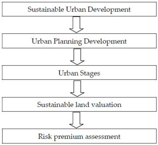
Figure 1.
Links between sustainable urban development and the risk premium for land valuation. Source: Own work.
Furthermore, land price fluctuation will significantly affect investment projects and so will have an important impact on the macroeconomy. Thus, we must be accurate in assessing land valuation. Currently, the most suitable method for land valuation when land is available for development is the dynamic residual method (DRM) [17,18], which is based on discounted cash flows (DCF) [19,20,21]. This methodology is based on the economic analysis of a real estate project to be developed over land that one wants to appraise. One of the most important parameters of this model is the risk premium used to calculate the discount rate [22,23,24,25].
The risk premium depends on the specific investment project. There is no rigorous historical database to calculate this parameter, because it depends on the concrete project risk [23,26]. In this sense, there is an evident difficulty in obtaining the necessary information of the other project risk premiums due to the reservations of the developers to make data on the returns of their projects available. This matter means that developers making appraisals do not have access to sufficient data to calculate the risk premium with the required rigor. Thus, the risk premium is assessed by the evaluation of factors that affect the specific investment project [22].
Because of that, the main aim of this article is to determine different risk premiums according to the urban stage of the land, as it increases along the execution of its urban plan. The estimation of risk premiums of each urban stage is realized by the assessment of the factors that affect the investment project risk [14,26]. The method used is the analytic hierarchy process (AHP) [27].
Each stage assumes a different investment project, and by association, a different risk premium is considered for each level [28]. In order to achieve this, in each development stage, a two-step model is established: The first one includes a qualitative analysis to obtain each risk level priority, and the second one includes another qualitative assessment for the global risk premium of the investment project. The goals of the first step are to identify the factors that influence the global risk of a real estate investment project [29,30], establish the different risk levels to be considered for an investment, and conduct a qualitative assessment for the prioritization of such risk levels. The goals of the second step are to conduct a qualitative assessment to obtain the project’s global risk premium as a function of the prioritization from the first step.
2. Materials and Methods
2.1. Data—Study Case
We targeted a study area in Badajoz, a town with a population of 150,000, in Southwest Spain, Southwest Europe. Badajoz is the most populated city in the Extremadura region. Figure 2 shows the location of Extremadura inside Spain as well as the administrative divisions of Extremadura and Badajoz inside Extremadura.
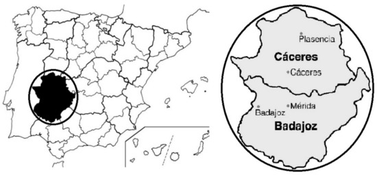
Figure 2.
Location of Extremadura in Spain. Administrative division of Extremadura and Badajoz. Source: Own work.
The municipal urban planning (MUP) of Badajoz was approved in 2007. This describes the general urban planning of the town in a technical document which establishes the directives of the urban development process and the design of land use. The study area covers land in the MUP named Sector SUB-CC-6.1–5 (Suelo Urbanizable con Condiciones nº 6.1-5—Urban Land for Development with Conditions nº 6.1–5). We show the location of the study area in Badajoz (Figure 3), an orthophoto-map (Figure 4), and boundaries Sector SUB-CC-6.1–5 (Figure 5).
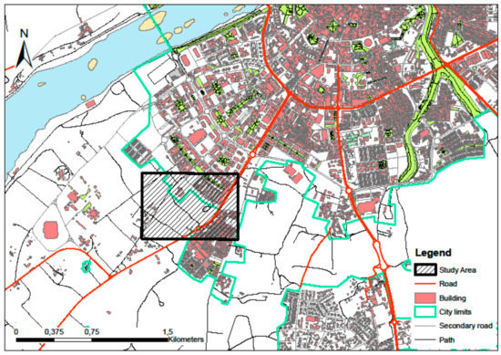
Figure 3.
Location of the study area and city limits. Source: Own work with GIS.
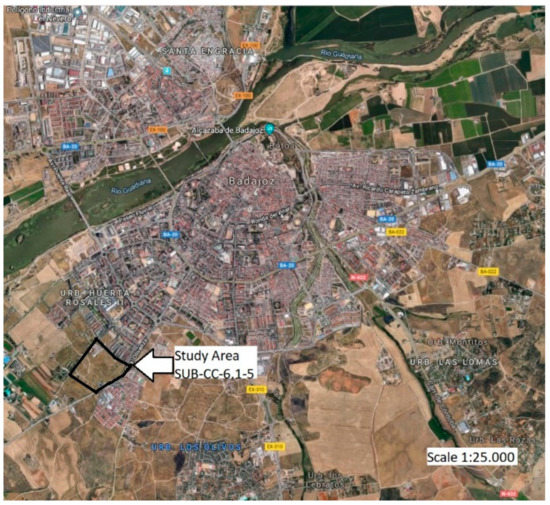
Figure 4.
Orthophoto map of the study area. Source: Orthophots Google, National Geography Institute.
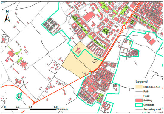
Figure 5.
Boundaries of the study area. Source: Source: Own work with GIS.
In Spain, the planning and spatial development law is different in each region, although, in any case, it is necessary to carry out an execution program (EP). In the MUP, the planning considerations in the analyzed area should be EP-approved through a document that establishes the detailed ordering design of the sector that is approved by the administration.
At the time of the study, the study area sector did not have an approved EP. In MUP, the EP must obey the urban use condition parameters displayed in Table 1. These parameters are mandatory. The table explains the coefficient values of each parameter related to sector buildability given in built square meters (bsm) divided by land square meters (lsm). In order to calculate the net area with urban use rights, the endowment of services public area must be defined in the gross area of the sector (Table 1).

Table 1.
Sector SUB-CC-6.1-5 urban use condition.
2.2. Methodology
2.2.1. Fundaments
The urban stages were determined according to the presence of an approved EP. In this study, four urban stages were considered: S1, the current stage of the selected land, corresponding to a limited area of developable land without an execution program; S2, the following stage, which considers the hypothesis of the land having an approved execution program; S3, the stage in which the hypothesis of the land being included in an actuation unit with approved reparceling is considered; and finally S4, corresponding to fully developed land on all its parcels. The overall estimated time horizon for the development of this methodology (from the urban state S1 to the final urbanized land S4) is 10 years [16].
In S1, S2, and S3, there is no physical transformation of the land; these stages are only different based on whether they have an approved EP document or not. There is only physical transformation is S4, in which the land is fully urbanized. Current, the land is in S1. The proposed model calculates the risk premiums for S1, S2, S3, and S4. Afterwards, by regression analysis, the graphic tendency and its formula are obtained. This is the equation that defines the evolution of the risk premium over time. For each urban stage, the project’s risk premium calculation method was divided in two steps: step one, the establishment of priorities for the different risk levels that the project can have, using the AHP model; and step two, quantifying the risk premium of each risk level, in order to assess the project’s global risk premium. An overview of the model is presented in Figure 6.
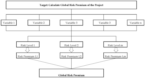
Figure 6.
Overview of the proposed model. Source: Own work.
This process was developed according to two phases:
2.2.2. First Phase: Risks Level Weighting
Considering the land valuation process aims to determine its price in a manner that the investment made by the building developer is profitable, during the decision-making process, and while assessing its profitability, it is essential to correctly identify the main risk factors that oppose the investor, as they are vital to the project’s viability. The supply and demand of the real estate being promoted along with physical, economical, and juridical factors will influence this risk. This is why specialized publications [31,32] as well as academic research from several authors [33,34] were used for the assessment of these risk factors.
The methodology used to establish the importance of the levels was based on the analytic hierarchy process (AHP), developed by Professor Saaty in the 1980s [27,35,36,37,38,39]. Through these methods, the different risk levels that the project can have were determined. At present, this methodology has been successfully used in various disciplines, such as education, economy, resource allocation, environmental applications, and also urban planning [40,41,42,43,44]. AHP’s potential is strong thanks to its multiple applications. In sum, AHP is a hypothesis selection model that is a function of its variables or criteria, which can have greater or lesser influence on the alternatives. It effectively uses a divide and conquer strategy, where the smaller tasks are combined to give a solution to the general problem. The explanatory variables are supplied by the different considered risk factors which influence the project, which are identified according to the previous paragraph. The goal is to find the best alternative. In order to do so, both the criteria and the alternatives are taken into account through a comparison of pair combinations in a matrix, judicious consideration of expert opinion on the subject, and a fundamental pair comparison scale. The reasoning behind comparing pairs is simplification—it is easier for the human brain to distinguish the best of two elements than to pick from a larger group, while having to ponder all the group’s characteristics simultaneously [45].
Having identified the criteria combined with the explanatory variables, the risk factors that can influence the investment building global risk can be characterized [34] and a hypothesis of the different risk levels that the investment project can have can be made [15,16].
To carry out the AHP, a group of experts was selected [27,41], in which all its members are endowed with the qualifications or the professional expertise regarding building and urban development. Contextually, 12 experts have been selected, and the inherent data are showing in the following (Table 2):
Table 2.
Experts group.
The expert´s perceptions were used to perform the analysis of the variables that influence the risk of investment. Each expert develops its hierarchy and makes its assessments—through the application of the geometric average, the group valuation results were obtained [42,46]. Therefore, the paired comparison matrix of the variables and the paired comparison matrices of the risk levels are formed.
Thus, the following 8 variables were selected [16]: V1, the land location; V2, the global sector use; V3, the average subjective use; V4, the urban development state; V5, the necessary amount of investment; V6, access to financing by potential buyers; V7, financial leverage of the investment project (30%) [16]; and V8, interest type. The analysis of the variables that influence the investment building risk [25,47] reported a paired comparison matrix, in which its elements represent the importance of each variable compared to the rest—according to the scale defined in Table 3. The eigenvector of this matrix indicates the weight that each variable has in the variables set [38].
Table 3.
Fundamental scale of pair comparisons.
On the other hand, 5 levels of risk were considered, from the minimum level to the maximum: RL1, RL2, RL3, RL4, and RL5. RL1 is related to the minimum level of risk estimated for the national sector of building contractors and RL5 to the maximum risk level [16]. The analysis of the influence of each variable on the different risk levels reports a pairwise comparison matrix of the risk level (PCMR) matrix for each variable. The eigenvector of each of these matrices gives us the weight that each risk level has—regarding the variable under analysis.
The process was developed by the follow steps:
- Criteria definition, which refers to the variables (Vi) which are assumed to have an influence on the global project risk;
- Determining a group of alternatives, which will determine the risk level (RL) which represents the different intensities the project is subject to;
- Establishing the pairwise comparison Matrix of the variables (PCMV). This is obtained through a comparison between pairs of variables, in which the pairs are individually compared according to the Saaty fundamental scale (Table 3).
The intermediate (even) values of the scale were used to qualify between two others of the fundamental scale.
To infer PCMV, variable V1 was initially compared to V1, V2, V3…Vn, and using the same logic, we iteratively compared V2 to V1, V2, V3…Vn. This occurred successively until Vn. In effect, by comparing a variable with itself, the quantifying value will be 1. The pair comparisons between each differing variable were based on the question “How much is variable Vx more influential than Vy in the project’s global risk?” Through these pair comparisons, PCMV was structured as a square matrix with n x n dimensions. The normalized eigenvector (EVV), associated with the greatest eigenvalue of the PCMV, indicated the pondered value of each variable in the set [38]. This assessment provided the relative relevance of each of them. In the following, the paired comparison matrix (PCMV) and its own vector (EVV) are obtained:
- 4.
- Establishing the pairwise comparison matrix of the risk level (PCMR): This was obtained by comparing the RLs, two by two, for each of the variables. This induced as many matrices as the number of considered variables. Like in the previous step, these comparisons were made with Saaty’s fundamental scale. With n variables, there would be the matrices PCMR1, PCMR2, PCMR3,…PCMRn squared with dimensions m x m, with m being the RL. The RL pair comparisons were based on answering the question “Given variable X, how much more influential is RLx than RLy?”
- 5.
- For each PCMRn matrix, we calculated its normalized eigenvector (EVR1, EVR2, EVR3…EVRn) to indicate the assessed risk levels according to the considered variable.
- 6.
- With the column matrices EVR1, EVR2, EVR3…EVRn of dimension (m x 1), from the previous step, a matrix of dimensions m xn was constructed (m being the RL and n being the number of Vi). This was the matrix of the risk level eigenvector (MRLE), with dimensions m x n.
- 7.
- The result of the product of MRLE (m x n) multiplied by EVV (n x 1) was a column matrix W (m x 1), whose elements indicated the weighting of the differing RLs of the project’s global risk.
Every pair comparison matrix had to adhere to the following conditions [42,48]:
- (a)
- Reciprocity: Si aij = x, => aji = 1/x.
- (b)
- Homogeneity: If the elements i and j were considered equally relevant and with the same weight, => aij = aji = 1, and furthermore, for every i => aii = 1, since every element compared with itself has equivalent relevance.
- (c)
- Consistency: This property was provided by the subjectivity of the expert opinion appraisal. Through the condition of consistency, this subjectivity was made as concretely as possible and thus needed to avoid inconsistencies that may arise from comparisons. The matrix had to be consistent. The matrix consistency was measured by the consistency ratio (CR). The maximum values for CR when the matrix was kept consistent and thus valid are presented in Table 4:
Table 4. Consistency ratio maximum percentages.
When an inconsistent matrix was obtained, consistency was improved until an acceptable consistency ratio that did not surpass the provided values of the previous table was obtained.
2.2.3. Second Phase: Global Risk Premium of Each Urban Stage
In order to assign a risk premium to the individual risk levels, a basis was established. A valid values range (VVR) was established, where the values of the risk premiums fluctuance in order that the investment building will be profitable were considered. Furthermore, it was estimated based on the expected returns on building development investments in Spain [49,50,51]. RL1 was linked to the minimum risk premium of the national sector of the building investment; RL5 was linked to the maximum risk premium possible in which the value for the building development investment is still profitable [15,16]. According to the abovementioned, the following VVR was estimated: minimum risk premium, RPmin = 8.00%; maximum risk premium, RPmax = 28.00%. Next, the different ranges amongst the VVR of RP were determined. Each of them corresponded to the individual risk levels that were considered. The estimated VVRs of the risk premiums for each level of risk are shown in the following table (Table 5):
Table 5.
Valid values range (VVR) of risk premium (RP) for each risk level.
The associate risk premiums (ARPi), for each RL were obtained by applying the weight of each of them (wi), to the valid range of each RL while linearly interpolating through weights. These weights were obtained from matrix (W) of each urban stage. The ARPi for each urban stage was obtained by the following formula:
with:
- ARPi, the value for the associated risk premium for each risk level;
- i, the risk level from 1 to 5;
- , the minimum value of the range for each risk level;
- , the maximum value of the range for each risk level;
- wi, the weight of each risk level, obtained from matrix W.
The risk premium for each urban state (RPS) is given by the following expression:
with:
- RPs, the risk premium for each urban state;
- i, the risk level from 1 to 5;
- ARPi, the value for the associated risk premium for each risk level.
- wi, the weight of each risk level, obtained from matrix W.
Thus, for the development of the model, the study was carried out considering a time horizon similar to those of other analyzed studies [16]; the point where the time horizon is 10 years and the time to get the different urban states (since S1) are presented in the following (Table 6):
Table 6.
Time to get the urban stage.
Through a linear regression analysis, we established the equation from the line that best fits the obtained results.
3. Results
3.1. Pairwise Comparison Matrix of the Variables (PCMV) and Eigenvctor (EVV)
It was estimated that the variables considered influenced all the urban states with the same weights, obtaining a single paired comparison matrix of variables (Table 7).
Table 7.
Pairwise comparison matrix of the variables (PCMV) and eigenvector (EVV).
3.2. Matrices of the Risk Level Eigenvector (MRLE) to Each Urban Stage
It was estimated that the risk levels were influenced differently in each urban state, obtaining a matrix of vectors of different levels of risk for each urban state (Table 8, Table 9, Table 10 and Table 11).
Table 8.
Matrix of the Risk Level Eigenvector (MRLE) for urban stage S1.
Table 9.
Matrix of the risk level eigenvector (MRLE) for urban stage S2.
Table 10.
Matrix of the risk level eigenvector (MRLE) for urban stage S3.
Table 11.
Matrix of the risk level eigenvector (MRLE) for urban stage S4.
3.3. Risk Level Weights on the Global Risk—W Matrix
The weight that each distinct risk level takes in terms of the projects’ global risk was provided by data from matrix W = (MRLE) x (EVV). The elements of this column in matrix W (5 x 1) express the relative weights of each RL. Thus, the weights of each risk level in the projects total risk are as follows: S1, risk level weights in Table 12; S2, risk level weights in Table 13; S3, risk level weights in Table 14; and S4, risk level weights in Table 15:
Table 12.
W Matrix—risk level weights for S1.
Table 13.
W Matrix—risk level weights for S2.
Table 14.
W Matrix—risk level weights for S3.
Table 15.
W Matrix—risk level weights for S4.
3.4. Global Risk Premium of each Urban Stage
Applying Formula (1), we obtain ARPi for Urban Stage S1:
Equally, we obtained the ARPi values for S2, S3, and S4.
Afterwards, by applying Formula (2), we obtained the global risk premium for each urban stage. The results are presented in the following tables (Table 16, Table 17, Table 18 and Table 19):
Table 16.
Global risk premium for S1.
Table 17.
Global risk premium for S2.
Table 18.
Global risk premium for S3.
Table 19.
Global risk premium for S4.
A summary of the risk premium results according to the urban stages is presented in the following (Table 20):
Table 20.
Summary of risk premium results according to the urban stages.
By regression linear analysis, the next figure (Figure 7) presents the model’s chart, which includes the tendency line obtained and the formula for the risk premium result as a function of the project’s progression year as an independent variable.
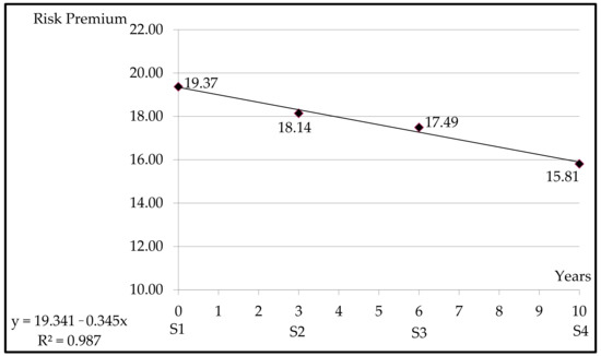
Figure 7.
Graphic and equation. Source: Own work.
By applying this model, we can calculate the risk premium value of a real estate investment project at any moment of urban planning development in order to assess any urban land for development in the same sector. The formula obtained to calculate the risk premium is the following:
where x is the year of urban planning development.
By applying the tendency line Formula (8) obtained, we present the risk premium values for each considered year in the following (Table 21):
Table 21.
Risk premium values according to the year of development of urban planning.
4. Discussion
In order to achieve rational growth and sustainable development in cities, it is very important to coordinate local policies for the development of municipal urban planning [52,53].
It was observed that a real estate investment project’s risk is influenced by many factors that affect both the systematic and nonsystematic risks. These factors materialize as a set of explanatory variables, which was considered in our case study [54]. The internal rate return is an index for evaluating and ranking investment projects. Recently, the selective internal rate of return, a criterion which selects an extended set of possible internal rates which can be used to evaluate projects, was introduced [55]. The main parameter to calculate this index is the risk premium of the investment project.
By applying the proposed model, the risk premium is obtained by a mathematical process which is valid and accurate. The results certify the validity of the model, as they are in a valid range of risk premium fluctuation according to Spanish real estate sector data [23,49]. The scientific rigor of this model emanates from the use of AHP, a method with widespread international adherence and acceptance as a support tool for assisted decision making and for establishing a specific selection of alternatives [27]. In our case study, information on risk factors was structured. Different weights were calculated for corresponding risk levels that the project is subject to. We also associated each risk level with a range of risk premium fluctuation for each stage. The partial risk premium for each level was also inferred. Finally, using all the above, we estimated the project’s global risk premium.
Risk premiums were calculated in four development urban stages [16] as a function of the specific point in the execution of urban planning: S1, developable land, delimited without an execution plan; S2, land with an approved execution plan; S3, land with an execution unit and approved reparceling; and finally, S4, fully developable land with completely urbanized parcels, ready to be built upon. For each of them, an accurate and scientifically rigorous risk premium was determined. The present work studied an overall time horizon of 10 years, from the current urban state (S1) to the final urbanized land (S4). The time horizons used in the present study are collected at Table 19. As an example, if there were changes in the times considered, there would also be changes in the function and, consequently, in the obtained results. Thus, the formula (8) could be used to perform different simulations depending on the time horizons considered.
The risk level weight results obtained for each urban stage imply that risk level 5 has the biggest value in S1 and risk level 1 has the biggest value in S4. This is due to the assumed risk in the real estate investment project being higher when the land does not have an execution program (S1) than when the land is fully urbanized and ready to be built (S4).
During urban stages S1, S2, and S3, there are no physical changes to the land. In these stages, there are only legal changes due to the progress of the administrative process related to the approval of the execution program and reparceling project documents. There are only physical changes to the land when moving from S3 to S4, when the land is just fully urbanized.
The global risk premium of each urban stage was obtained by applying the weighted average of the risk level weights obtained by AHP according to eight estimated variables which the expert panel considered as being most influential factors on the development of urban planning. This analysis showed that the risk premium in stage S4 is around 20% smaller than the risk premium in S1.
The risk premium results obtained for each urban stage are in the valid range of risk premiums estimated for both the national and local real estate markets [49].
Therefore, the novelty of this paper is based on the following aspects:
- 8.
- With the proposed model, the risk premium can be determined for the valuation of developable land. Furthermore, this model can be used in cases where historical profitability data of similar projects are not available. This is quite usual, given that developers are reluctant to offer the profitability data obtained in their investment projects. The risk premium must be estimated by evaluating the factors that influence the risk of the specific investment project [22,23].
- 9.
- The variation in the risk premium is considered based on the development of urban planning over time. This aspect is based on the fact that as urban planning develops, the risk of the investment project varies, since the time horizon is a variable that influences the assumed risk level [33].
The proposed model was applied to a sector of developable land in the city of Badajoz, Spain. The model can easily be applied to any developable land in Spain or in other country. In fact, starting from the risk factors that influence the assessment of land to be valued, paired comparison matrices are formed, and the level of risk of the investment project, depending on the variables under consideration, is determined following the methodology [27]. To set the valid range of values (VVR) of the risk premium (see Section 2.2.3 of the present work), it is necessary to establish the maximum and minimum values estimated for the country under evaluation.
Effectively, in this paper, it was observed that when the dataset on other projects’ risk premiums is small, the proposed model is a valid and scientifically rigorous method that can be used to estimate a specific real estate project’s future risk premium. This model provides the weight of each risk level. Subsequently, instead of picking the alternative with the most weight, we opted to process the weighted average of each weight’s value in order to get the end result. From the identification of the project’s risk factors, the global risk premium is obtainable [23]. Once obtained, it is ready to be used for assessing potentially developable land.
The proposed method is an alternative to the classic models for estimating the risk premium. The most used are the one based on historical data from similar projects [56]; the one based on direct surveys to experts [57,58]; and the Capital Assets Pricing Model (CAPM) [19,59]. The models based on historical data and exploratory tools as the survey method are, today, a base of several discussions among academicians [22,23,56], due to the fact that investors do not have the same expectations of profitability and risk and, therefore, each project needs to be analyzed individually. On the other hand, the CAPM model starts from the premise that there is investment diversification; however, when valuing a land using the flow rate discount model, in fact, we are valuing a specific investment project, and consequently, there is no diversification in the investment. Therefore, there would be more rigor if the estimate was in the risk presented in the variables that affect the investment project [26,60].
The obtained results, in comparison with other analyzed works carried out in nearby areas in the same city, are similar [15,16], all being within the range of a valid value defined for the risk premium of the investment building. Thus, analyzing the obtained results, it is possible to verify that they are within the range of values collected in other works for the investment building in Spain [49,50,51]. In addition, if we compare the obtained results with the other studies conducted on the Spanish risk premium market [57], it is possible to realize that the results for the risk premium of the investment project in the study area are higher—presenting an excess risk premium, considering the Spanish market.
With this in hand, the risk premium at any stage of execution is easily inferable, as shown by the straight line presented in Figure 5. It must be stated that, despite higher risks usually offering higher profitability, given a similar straight line with an acute incline, the risk premium would increase significantly. Under these conditions, inconsistency in the net present value of the project could be implied, and consequentially, it would become unfeasible [55].
It has been reasoned from the obtained results that one of the risk premium’s most influential factors is the urban stage of the land, as identified according to its urban development planning time. Gathered data show that this variable impacts the risk level decisively.
This paper shows that the risk premium decreases during urban planning development. In other words, it is much larger in the initial stage (S1), when the land has no execution program, and decreases as it approaches S4, the final stage. The regression linear analysis (Figure 7) shows the risk premium variation during urban planning development. The regression results show a very high correlation with good adjustment, so the risk premium variation can be explained by the equation of the straight line obtained.
Once the graphic equation is obtained, the way to apply this model is, first, to establish the current time of the urban stage, and second, to apply the graphic equation. This can calculate the risk premium value of a real estate investment project at any moment of urban planning development to assess any urban land for development in the same sector.
This model is a good alternative for calculating the risk premium of a real estate investment project in a scientific and mathematical way [22]. The main constraint could be that the results are only valid for a certain period of time during which the economic and financial variables do not change significantly [30]. Following changes, a new analysis of the variables must be done.
As a possibility for future research, we point to the study of other factors that could influence the risk of the investment project based on different economic indicators of the country where it is being applied. This work can help to determine the land value into the scope of other studies’ research linked with smart city services [61].
5. Conclusions
A model that represents a solid alternative for risk premium assessment using scientific, technical, and mathematical approaches was presented. This study makes the following main conclusions:
- The urban stage is one of the most influential factors in the risk premium value.
- The risk premium for a land for development varies depending on the urban state in which the land is inserted by the time of the valuation. It is decreasing as the development of urban planning that affects the sector progresses.
- In the case study, and based on the obtained results, the variables that most influence the determination of the risk premium are: V6, access to financing; followed by V8, the interest rates. On the other hand, the variables that less influence the determination of the risk premium are: V7, financial leverage of the investment; followed by V3, average subjective use of the sector.
- We can calculate the risk premium at any moment during urban planning development. In fact, Equation (7) is used to calculate the risk premium for the valuation of any developable land within the same sector of the city—depending on the year after which the urban planning that affects this sector begins to develop. The value of the risk premium when the land is urbanized (S4) represents 81.62% of the value at the initial moment (S1)—when the land has no execution program.
- The presented methodology can be replicated in other areas, obtaining, however, different results based on the analysis of the influence on risk and which variables are considered.
- With this model, we can assess the risk premium for the valuation of urban land for development, without needing historic data on project returns; these data can be deceptive because they are related to a previous time.
Author Contributions
Conceptualización, J.M.C.R.; Methodology, J.M.C.R.; software, J.M.C.R.; Validation, J.M.C.R.; Formal analysis, J.M.C.R.; Investigation, J.M.C.R.; Resources, J.M.C.R.; Data curation, J.M.C.R.; Writing-original draft preparation, J.M.C.R.; Writing-review and editing, J.M.N.G. and R.A.C.; Visualization, J.M.N.G. and R.A.C.; Supervision, J.M.N.G., R.A.C. and J.C.F.; Project administration, J.C.F.; Funding acquisition, J.C.F.
Funding
This research received no external funding.
Acknowledgments
The publication of the present work was possible thanks to funding granted by the European Regional Development fund (FEDER in Spanish) and by the Board of Extremadura to the Research Group of Sustainable Development and Territorial Planning through the financial help of reference GR18052 and the Environmental Resources Analysis Research Group through the financial help of reference GR18054.
Conflicts of Interest
The authors declare no conflict of interest.
References
- Naess, P. Urban Plannign and Sustainable Development. Eur. Plan. Stud. 2001, 9, 503–524. [Google Scholar] [CrossRef]
- Tosics, I. European urban development: Sustainability and the role of housing. J. Hous. Built Environ. 2004, 19, 67–90. [Google Scholar] [CrossRef]
- Yigitcanlar, T.; Teriman, S. Rethinking sustainable urban development: Towards an integrated planning and development process. Int. J. Environ. Sci. Technol. 2015, 12, 341–352. [Google Scholar] [CrossRef]
- Nooten, G.A. Sustainable development and Nonrenewable resources. A multirateral perspective. In Proceedings, Workshop on Deposit Modeling, Mineral Resource Assessment and Sustainable Development; USGS: Reston, VA, USA, 2007; pp. 35–40. [Google Scholar]
- Berges, A.; Ontiveros, E. La nueva ley del suelo desde la perspectiva económica. Sostenibilidad y eficiencia en los mercados del suelo. Ciudad Territ. 2007, 29, 259–275. [Google Scholar]
- Chirstensen, F.K. Understanding value changes in the urban development process and the impact of municipal planning. Land Use Policy 2014, 36, 113–121. [Google Scholar] [CrossRef]
- Kalbro, T.; Lindgren, E. Markexploaterin, 4th ed.; NorstedtsJurikik: Stockholm, Sweden, 2010. [Google Scholar]
- Williamson, I.; Enemark, S.; Wallace, J.; Rajabifard, A. Land Administration for Sustainable Development; Esri Press: Redlans, CA, USA, 2010. [Google Scholar]
- Bruton, M.; Nicholson, D. Local Planning in Practice; Routledge: London, UK, 2013; ISBN 9781135883249. [Google Scholar]
- Mayer, C.J.; Somerville, T.C. Land use regulation and new construction. Reg. Sci. Urban Econ. 2000, 30, 639–662. [Google Scholar] [CrossRef]
- Gyourko, J.; Saiz, A.; Summers, A. A New Measure of the Local Reguatory Environment for Housing Markets: The Wharton Residential Land Use Regulatory Index. Urban Stud. 2008, 45, 693–729. [Google Scholar] [CrossRef]
- Seto, K.C.; Dhakal, S.; Bigio, A.; Blanco, H.; Delgado, G.C.; Dewar, D.; Huang, L. Human Settlements, Infrastructure and Spatial Planning; Mitigation of Climate Change; IPCC Working Group III Contribution to AR5; Cambridge University Press: Cambridge, UK, 2014; Chapter 12. [Google Scholar]
- Caparros, A. Valoración de Suelos; Aranzadi: Madrid, Spain, 2012. [Google Scholar]
- Wyatt, P. Property Valuation, 2nd ed.; John Wiley & Sons, Inc.: New York, NY, USA, 2013. [Google Scholar]
- Codosero, J.M.; Cabezas, J.; Castanho, R.A.; Naranjo, J.M. Estimación de la prima de riesgo para la valoración del suelo con aprovechamiento urbanístico: Un caso de estudio. Suelo urbanizable en Badajoz, España. Monfragüe Desarro. Resiliente 2017, 8, 60–74. [Google Scholar]
- Codosero, J.M.; Naranjo, J.M.; Castanho, R.A.; Cabezas, J. Land Valuation Sustainable Model on Urban Planning Development: A Case Study in Badajoz, Spain. Sustainability 2018, 10, 1450. [Google Scholar] [CrossRef]
- Scarret, D.; Osborn, S. Property Valuation: The Five Methods; Routledge Taylor and Francis Group: New York, NY, USA, 2014. [Google Scholar]
- European Group of Valuers Asociation. European Valuation Standards; Gillisnv/sa: Brussels, Belgium, 2016. [Google Scholar]
- Damodaran, A. Investment Valuation. Tools and Techniques for Determinig the Value of Any Asset; John Wiley & Sons, Inc.: New York, NY, USA, 2012. [Google Scholar]
- Steiger, F. The Validity of Company Valuation Using Discounted Cash Flow Methods. arXiv 2008, arXiv:1003.4881. [Google Scholar]
- De Andrés, P.; De Fuente G y San Martín, P. Capital budgeting practices in Spain. Bus. Res. Q. 2015, 18, 37–56. [Google Scholar] [CrossRef]
- Shilling, J.D. Isthere a risk premiun puzzle in real estate? Real Estate Econ. 2003, 31, 501–525. [Google Scholar] [CrossRef]
- Fernández, P. La Prima de Riesgo del Mercado; Documento de Investigación, DI-585: 1-33; IESE Business School, Universidad de Navarra: Barcelona, Spain, 2005. [Google Scholar]
- Hammond, P.B.; Leibowitz, M.L.; Siegel, L.B. Rethinking the Equity Risk Premium; Research Foundation of Chartered Financial Analyst Institute: Charlotte Town, VA, USA, 2011; ISBN 978-1-934667-44-6. [Google Scholar]
- D’Amato, M.; Kauko, T. Mass Appraisal Methods: Na International Perspective for Property Valuers; Wiley-Blackwell: San Francisco, CA, USA, 2008. [Google Scholar]
- Isaac, D.; O’Leary, J. Property Valuation Principles; Palgrave Macmillan: London, UK, 2012. [Google Scholar]
- Saaty, T.L. Decision making with the analytic hierarchy process. Int. J. Serv. Sci. 2008, 1, 83–98. [Google Scholar] [CrossRef]
- Contreras, C. Value for money: To what extent does discount rate matter? Rev. Econ. Apl. 2014, 66, 93–112. [Google Scholar]
- Edelstein, R.H.; Magin, K. The Equity Risk Premium for Securitized Real Estate: The Case for U.S. Real Estate Investment Trusts. J. Real Estate Res. 2013, 35, 393–406. [Google Scholar]
- D’Alpaos, C.; Canesi, R. Risks Assessment in Real Estate Investments in Times of Global Crisis. WSEAS Trans. Bus. Econ. 2014, 11, 369–379. [Google Scholar]
- International Valuation Standards Council. International Valuation Standards; International Valuation Standards Council: London, UK, 2017. [Google Scholar]
- Asociación Española de Análisis de Valor. Criterios Técnicos Dirigidos a la Armonización de las Prácticas Profesionales y de los Parámetros Relevantes para la Aplicación de los Métodos de valor Residual a la Valoración de Suelos Urbanos o Urbanizables; AEV: Madrid, Spain, 2014. [Google Scholar]
- Michel, G. Real Estate Risk in Equity Returns: Empirical Evidence from U.S. Stock Markets; European Business School, Springer Science and Business Media: Berlin/Heidelberg, Germany, 2009; ISBN 9783834994967. [Google Scholar]
- Parker, D. Global Real Estate Investment Trusts; John Wiley & Sons: San Francisco, CA, USA, 2012. [Google Scholar]
- Saaty, T.L. The Analytic Hierarchy Process; McGraw Hill: New York, NY, USA, 1980. [Google Scholar]
- Saaty, R.W. The Analytic Hierarchy Process-What it is and how it is used. Math. Model. 1987, 9, 161–176. [Google Scholar] [CrossRef]
- Saaty, T.L. Howtomake a decision: The Analytic Hierarchy Process. Eur. J. Oper. Res. 1990, 48, 9–26. [Google Scholar] [CrossRef]
- Saaty, T.L. Decision-making with the AHP: Why is the principal eigenvector necessary. Eur. J. Oper. Res. 2001, 145, 85–91. [Google Scholar] [CrossRef]
- Saaty, T.L.; Vargas, L.G. Decision Making with the Analytic Network Process: Economic, Political, Socialand Technological Applications with Benefits, Opportunities, Costs and Risks; Springer: New York, NY, USA, 2006. [Google Scholar]
- Martín, L.; De la Torre, C. Valoración de Riesgos de un Proyecto Utilizando el Proceso Jerárquico de Análisis; Asociación Española de Profesores Universitarios de Matemáticas para la Economía y la Empresa. VI Jornadas; Área de Matemáticas, Facultad de Ciencias Jurídicas y Sociales, Universidad de Castilla: La Mancha, Spain, 1998. [Google Scholar]
- Vaidya, O.S.; Kumar, S. Analytic hierarchy process: An overview of applications. Eur. J. Oper. Res. 2006, 169, 1–29. [Google Scholar] [CrossRef]
- Aznar, J.; Guijarro, F. Nuevos Métodos de Valoración. Modelos Multicriterio; Editorial Universidad Politécnica: Valencia, Spain, 2012. [Google Scholar]
- González-Ramiro, A.; Gil Gonçalves, A.; Sanchez-Ríos, A.; Jeong, J.S. Using a VGI and GIS-Based Multicriteria Approach for Assessing the Potencial of Rural Tourism in Extremadura, Spain. Sustainability 2016, 8, 1144. [Google Scholar] [CrossRef]
- Sdino, L.; Rosasco, P.; Magoni, S. Real Estate Risk Analysis: The Case of Caserma Garibaldi in Milan. Int. J. Financ. Stud. 2018, 6, 7. [Google Scholar] [CrossRef]
- Arrow, K.J.; Raynaud, H. Social Choice and Multicriterion Decision-Making; The MIT Press: Cambridge, MA, USA, 1986. [Google Scholar]
- Dong, Y.; Zhang, G.; Hong, W.C.; Xu, Y. Consensus models for AHP group decision making under row geometric mean prioritization method. Decis. Support Syst. 2010, 49, 281–289. [Google Scholar] [CrossRef]
- Adair, A.; Downie, M.L.; McGreal, S.; Vos, G. European Valuation Practice: Theory and Thechniques; Taylor & Francis: New York, NY, USA, 2013. [Google Scholar]
- Brunelli, M.; Canal, L.; Fedrizzi, M. Inconsistency indices for pairwise comparison matrix: A numerical study. Ann. Oper. Res. 2013, 211, 493–509. [Google Scholar] [CrossRef]
- Antuña, R. Protocolos para la Definición del Proyecto Inmobiliario Óptimo Mediante el Análisis de los Riesgos Vinculados al Activo Inmobiliario. Ph.D. Thesis, Universidad de La Coruña, La Coruña, Spain, 2015. [Google Scholar]
- Solvia Market View. Tendencias del mercado inmobiliario. Solvia 2017, 4, 1–31. [Google Scholar]
- Ratios Sectoriales de Sociedades no Financieras. Available online: http://app.bde.es/rss_www/Ratios (accessed on 11 July 2019).
- Kaufmann, V.; Sager, F. The coordination of local policies for urban development and public transportation in four swiss cities. J. Urban Aff. 2006, 28, 353–373. [Google Scholar] [CrossRef][Green Version]
- Engelman, R. Is Sustainability Still Possible? Island Press: Washington, DC, USA; London, UK, 2013; Chapter 1; pp. 3–19. [Google Scholar]
- Tsai, H.-F.; Luan, C.-J. What makes firms embrace risks? A risk-taking capability perspective. Bus. Res. Q. 2016, 19, 219–231. [Google Scholar] [CrossRef]
- Weber, T.A. On the (non-)equivalenceof IRR and NPV. J. Math. Econ. 2014, 52, 25–39. [Google Scholar] [CrossRef]
- Ibbostson, R.G. The Equity Risk Premium; The Research Foundation of CFA Institute: Charlotte Town, VA, USA, 2011; pp. 18–26. ISBN 978-1-934667-44-6. [Google Scholar]
- Fernández, P.; Pershin, V.; Fernandez, I. Discount Rate (Risk-Free Rate and Market Risk Premium used for 41 countries in 2017: A survey. IESE Bus. Sch. 2017. [Google Scholar] [CrossRef]
- Psunder, I.; Cirman, A. Discount rate when using methods based on discounted cash flow for the purpose of real estate investment analysis and evaluation. Geod. Vestnik 2011, 55, 561–575. [Google Scholar]
- Brealey, R.; Myers, S.; Allen, F. Principles of Corporate Finance; McGraw-Hill Irwin: New York, NY, USA, 2011. [Google Scholar]
- Contreras, E.; Cruz, J.M. No más VAN: Value at Risk del VAN, una nueva metodología para el análisis de riesgo. Rev. Trend Manag. 2006, 8, 1–17. [Google Scholar]
- Miltiadis, D.L.; Visvizi, A.; Sariete, A. Clustering Smart City Services: Perceptions, Exceptations, Responses. Sustainability 2019, 11, 1669. [Google Scholar]
© 2019 by the authors. Licensee MDPI, Basel, Switzerland. This article is an open access article distributed under the terms and conditions of the Creative Commons Attribution (CC BY) license (http://creativecommons.org/licenses/by/4.0/).