Impact of Influencing Factors on CO₂ Emissions in the Yangtze River Delta during Urbanization

Abstract

The Yangtze River Delta (YRD) is China’s largest urban agglomeration with a rapid urbanization process. This paper analyzes the dynamic relationship between urbanization rate, energy intensity, GDP per capita, and population with CO₂ emissions in YRD over 1990–2011 based on the extended STIRPAT model, impulse response function, and variance decomposition. A support vector machine model was constructed to further predict the scenarios of YRD’s CO₂ emissions from 2015–2020. The results show that YRD’s CO₂ emissions continuously increased during the sample period and are predicted to increase over 2015–2020. Energy intensity is the most influential factor, both in the short and long term, and the total population contributes the least. However, the influencing magnitude of energy intensity tends to decrease in the long term. The increase of urbanization rate is still accompanied by the increase of CO₂ emissions in YRD, but an inverted-U shape relationship between them may exist in the long term. The contribution of GDP per capita to CO₂ emissions is higher than the population and urbanization rate, and its contribution rate for CO₂ emissions is growing. The Kuznets curve does not exist in the current YRD.

1. Introduction

1.1. Research Background

Cities are the center of energy consumption, and environmental pressure will become more severe during the urbanization process (Al-Mulali et al., 2013; Chikaraishi et al., 2015) [1,2]. According to IEA (2008) [3], more than 66% of the world’s energy is consumed by urban demand and 70% of CO₂ emissions are contributed by cities.

China, one of the largest developing countries, is experiencing rapid urbanization. From 1978–2017, its urbanization rate rose from 17.92–58.52 percent (NBS, 2018) [4]. This may be the main reason for and background behind the sharp increase of energy consumption and related CO₂ emissions in China. Gregg et al. (2008) [5] pointed out that China had become the largest emitter of CO₂ emissions in 2006. To address the severe environmental problems, the National Development and Reform Commission released China’s new urbanization plan (2014–2020), which advocates the concept of an ecological civilization and calls for the formation of low-carbon production mode and lifestyle during the urbanization process.

However, the regional urbanization process is very imbalanced in China, and CO₂ emissions present different characteristics in different regions because of different urbanization rates and the regional development model (Shen et al., 2005; Zhang and Lin, 2012; Lin et al., 2017) [6,7,8]. That means the country-level recommendations are not very instructive for regional low-carbon development. Therefore, it is necessary to choose a specific region as the research object so as to realize the dual strategies of urbanization and the transition to a low-carbon economy in China.

This paper aims to explore the influencing factors and characteristics of YRD’s CO₂ emissions during its urbanization processes. YRD was selected for the following reasons. First, as China’s largest urban agglomeration, YRD plays an important strategic role in the national economic development and urbanization process. In 2017, YRD contributed 20.5 percent of national GDP and nearly 35.3 percent of China’s imports and exports (NBS, 2018) [9]. President Xi declared at the China International Import Expo in 2018 that YRD’s regional integration has risen to the national strategy. According to the Outline of the Yangtze River Delta Regional Integration Development Planning issued in 2019, the regional integration of YRD mainly refers to regional cooperation in some key areas such as coordinated regional development, collaborative innovation, infrastructure, ecological environment, public services, opening-up, and unified market. Second, YRD’s ecosystem function and environmental quality have been deteriorating during the urbanization. The fast-growing economy and energy-intensive industries resulted in huge energy consumption. Its total primary energy consumption reached 643.19 million tons of standard coal equivalent in 2017, which accounted for 14.33 percent of the whole nation (NBS, 2018) [9]. Such a huge energy consumption brings about considerable CO₂ emissions and serious air pollution. According to the “Development plan of Yangtze River Delta Urban Agglomeration” issued by the State Council in 2016, the number of days in which air quality reached the healthy standard was less than 250 days in the whole year. Therefore, analyzing the characteristics of emissions and future potential scenarios during the urbanization can not only help mitigate the tremendous environmental pressures in YRD, but also have a crucial instructive role in China’s low-carbon urbanization.

1.2. Contributions of this Paper

Research into the relationship between urbanization and CO₂ emissions has attracted significant attention (Chikaraishi et al., 2015; Bekhet and Othman, 2017; Martínez-Zarzoso and Maruotti, 2011) [2,10,11]. These studies mainly focused on answering three questions: influencing factors, correlation, and magnitude (Shi and Li, 2018) [12]. The influencing factors involve urbanization itself and its mechanism on CO₂ emissions such as the economy, population, technology, lifestyle, industry structure, transportation, and urban planning (Chikaraishi et al., 2015; Madlener and Sunak, 2011) [2,13]. For example, Yang et al. (2015) [14] found that urbanization would result in population concentration and a more carbon-intensive urban lifestyle. Wang et al. (2019) [15] adopted a factor-reversible structural decomposition method to analyze the impact of urbanization on carbon emissions in China. The results showed that urbanization changed the consumption pattern, and the transportation sector became one of the largest emission sectors. Azizalrahman and Hasyimi (2019) [16] classified the urban sector drivers of CO₂ emissions into residential, commercial, and industrial factors and examined their different roles in different income-level countries.

Studies on the correlation and magnitude are mainly empirical research. A variety of approaches or models are adopted, and the logarithmic division decomposition index method (LMDI), the IPAT or STIRPAT model, and Kaya and U-Kaya (introducing the urbanization factor into the Kaya Identity) are the most-used classical models. However, huge differences exist in the research findings in this field (Wang et al., 2016) [17]. For instance, as for the factor of economic development, Sharma (2011) [18] and Zhang et al. (2017) [19] both found that GDP per capita had a significant positive effect on CO₂ emissions. However, Azizalrahman and Hasyimi (2019) [16] found that GDP per capita only presented positive correlations with CO₂ emissions in upper-middle and lower-middle income countries, and the correlation was negative in high income countries.

As to the factor of urbanization, Sharma (2011) [18] used dynamic panel data of 69 countries from 1985–2005 and found that the influence of urbanization on CO₂ emissions was negative and statistically insignificant. Yao et al. (2018) [20] employed the threshold regression model and also found that urbanization can reduce the CO₂ emissions in China. However, the reducing role is diminishes with the increase of the urbanization rate. In contrast, Zhang and Lin (2012) [7] used the STIRPAT model based on panel provincial data from 1995–2010 in China and found that urbanization continuously increased CO₂ emissions. Zhu et al. (2012) [21] used a panel of 20 emerging countries from 1992–2008 and found that an inverted U-shaped curve did not exist between urbanization and CO₂ emissions. Shahbaz et al. (2017) [22] found that there existed a U-shaped relationship between urbanization and CO₂ emissions in Malaysia based on the STIRPAT model using the data from 1970–2011.

The related literature review revealed that the influencing factors of CO₂ emissions demonstrate obvious geographical characteristics and country-level differences. Many kinds of effects exist along with the urbanization process, which bring about different influences on CO₂ emissions. Therefore, further empirical research on urbanization and CO₂ emissions is still needed, even if they have been widely studied. Some scholars further pointed out that countries that are experiencing a rapid urbanization process should be given more attention (Wang et al., 2016) [17]. In this context, studies on China, a large and developing country with a rapid urbanization process, have increased in recent years (Sheng and Guo, 2016; Wu et al., 2017; Yang et al., 2018) [23,24,25]. However, these studies mainly focus on the country or industrial levels, and few investigate the influence of urban agglomeration regions such as YRD (Ouyang et al., 2018) [26]. Ouyang et al. (2018) [26] analyzed YRD’s energy rebound effect and found that the rebound effect of the industrial sectors was as high as 40.04%. Li et al. (2018) [27] analyzed YRD’s CO₂ emissions efficiency, which is “the ratio of the target CO₂ emissions to the actual CO₂ emissions, and the target CO₂ emissions can be calculated by data envelopment analysis (DEA) model”. However, neither of the above two studies comprehensively considered the influencing factors of CO₂ emissions. Song et al. (2015) [28] and Zhu et al. (2017) [29] used the LMDI model to analyze the influencing effect of energy-related carbon emissions in YRD. However, they did not consider the impact of urbanization on CO₂ emissions and did not analyze the dynamic effects of different factors. Considering the crucial roles of YRD in the Chinese low-carbon urbanization process, this scarcity would influence the effectiveness of policies.

To fill in this research gap and contribute to the literature in this field, this paper proposes an extended STIRPAT model to measure the influencing factors on CO₂ emissions under the background of YRD’s urbanization. Considering data availability and the focus on the fastest urbanization phase, our study selected the period from 1990–2011. Different from most existing literature, the contributions of this paper are two-fold: (1) In order to comprehensively analyze YRD’s CO₂ emissions, we combine the STIRPAT model, the vector autoregression (VAR) model, the impulse response function (IRF), and variance decomposition (VD) to analyze the cointegration and dynamic correlation between CO₂ emissions and different factors, as well as the impact magnitude of each factor. (2) We construct the support vector machine (SVM) model based on the influencing factors to predict the different emission scenarios of YRD. In order to improve the accuracy of forecasting, the future values of all the influencing factors are defined based on the government policy goals. The results obtained from the above models will be useful for YRD’s governments to formulate effective policies and better deal with the emissions pressure during the urbanization.

The rest of the paper is organized as follows: Section 2 describes the models and methodology of STIRPAT, VAR, IRF, VD, and SVM. Section 3 introduces the study area and data source. Results and discussions are presented in Section 4 and Section 5. Finally, the conclusions are summarized in Section 6.

2. Methodology

2.1. STIRPAT Model

Ehrlich and Holdren (1971) [30] proposed the IPAT model to explain the impact of human activities on the environment. The model can be described as I = PAT, where I denotes the environmental pressure, P represents the population, A represents affluence, and T is technology. This model has been considered a useful analytical tool to study the relationship between urbanization and environmental pressure (Shahbaz et al., 2017) [22]. However, it has some limitations, which we will not present here. Based on this model, Dietz and Rosa (1997) [31] and York et al. (2003) [32] developed the STIRPAT model, which can be expressed as:

$$I_i=\alpha P_i{}^{\beta }{A}_i{}^{\gamma }{T}_i{}^{\delta }{e}_i,$$

(1)

where I_i, P_i, A_i, and T_i have the same meanings as the original IPAT model, α, β, γ, and δ are estimated parameters, and e_i is the random error. After taking the logarithm of both sides of Equation (1), the model is transformed into a linear equation:

$$\ln \left(I_i\right)=\alpha +\beta \ln \left(P_i\right)+\gamma \ln \left(A_i\right)+\delta \ln \left(T_i\right)+e_i,$$

(2)

where α and e_i are the Napierian logarithms of α and e_i in Equation (1). β, γ, and δ reflect the elasticity relationship, i.e., the percentages of environmental change, which are caused by one percentage in one of the influencing factors when the others stay the same.

The STIRPAT model allows additional factors to be added as long as they are conceptually consistent with the multiplicative specification described in Equation (1). It has become one of the classical models to examine the influencing forces of CO₂ emissions. To further our analysis, we extended the STIRPAT model by incorporating urbanization level into it. Referring to previous literature, the specific extended model is shown as:

$$CARBO{N}_t={\alpha }_t{ENERTEN}_t^{\beta }{PERGDP}_t^{\gamma }{POPULATION}_t^{\delta }{URBAN}_t^{\lambda }{e}_t,$$

(3)

where CARBON denotes the CO₂ emissions (environmental pressure), PERGDP is GDP per capita, which stands for the economic development level or affluence, POPULATION and URBAN represent the total population size and urbanization rate, respectively, ENERTEN refers to energy intensity (technology level), and t represents time. Taking logs, Equation (3) can be converted to the logarithmic form:

$$\ln CARBO{N}_t={\alpha }_t+\beta \ln ENERTE{N}_t+\gamma \ln PERGD{P}_t+\delta \ln POPULATIO{N}_t+\lambda \ln URBA{N}_t+e_t$$

(4)

2.2. Vector Autoregression Model

The VAR model is formulated by taking every endogenous variable in the system as the function of lagged values of the endogenous variables themselves (Sims, 1980) [33]. This model is mainly employed to “analyze and predict the dynamic impact of systematic random disturbance, the magnitude and nature of the effect and the sustained time” (Hao et al., 2018) [34]. It provides a useful tool for analyzing the dynamic influence among the variables of one system. The mathematical expression of the VAR model is as follows (Talbi, 2017; Chi et al., 2017) [35,36]:

$$Y_t=\alpha +A_1{Y}_{t-1}+A_2{Y}_{t-2}+\cdots +A_p{Y}_{t-p}+{\epsilon }_t$$

(5)

In this paper, Y_t is a vector consisting of 5 endogenous variables as Y_t = (CARBON_t, ENERTEN_t, PERGDP_t, URBAN_t), where A₁, A₂$\cdots$A_p are the parameter matrix, and ε_t is the disturbance vector.

2.3. IRF and VD

In the VAR model, “when the disturbance term of an endogenous variable is plus one-unit or one-unit of standard deviation while other disturbance terms of endogenous variables remain constant, the corresponding value of the explanatory variable is called impulse response function” (Olson et al., 2014) [37]. In IRFs, the shock on one variable will not only influence this variable itself, it also can pass to other endogenous variables through the dynamic structure of VAR. As such, IRF can measure the current and future values of variables in the system when there is a standard deviation shock of a random disturbance term. The vector moving average (VMA) can be obtained from Equation (5) (Wang et al., 2018) [38]:

$$Y_t={\phi }_0{\epsilon }_t+{\phi }_1{\epsilon }_{t-1}+{\phi }_2{\epsilon }_{t-2}+\cdots +{\phi }_p{\epsilon }_{t-p}+\cdots$$

(6)

where φ_p = (φ_p,ij) are coefficient matrixes, p = 0, 1, 2 $\cdots$. The response function of y_i, which is caused by the impulse of y_i, is φ_0,ij, φ_1,ij, φ_2,ij $\cdots$.

VD provides another approach to describe the system dynamics compared to IRF. It is mainly utilized to analyze the contribution of each structural shock to the change of the endogenous variables, often estimated by variance (Sims, 1980) [33]. By decomposing the mean squared error of the whole system into the contribution of shocks on each variable, variance can help to understand the relative significance of each random disturbance’s effect.

2.4. SVM

The SVM was proposed by Cortes and Vapnik (1995) [39], which is a supervised machine learning approach based on the VC dimension (for Vapnik–Chervonenkis dimension) of statistical learning theory and the structural risk minimization principle. It can overcome some traditional difficulties including dimension disaster and over learning (Wang et al., 2018) [40] and thus out-performs similar methodologies such as the classical statistical model (Mladenović et al., 2016) [41]. For non-linearly-separable problems, the core idea of an SVM is mapping the input variables of a low-dimensional space into a high-dimensional feature space to find an optimal hyper-plane. For mathematical equations of SVMs, readers can refer to Li et al. (2018) [42] and Wang et al. (2018) [38].

3. Study Area and Data Source

3.1. Study Area

YRD, the largest urban agglomeration in China and the sixth largest urban agglomeration in the world, includes Shanghai city, Zhejiang province, and Jiangsu province. It is one of the most prosperous regions, and the urbanization process of YRD is very fast. Moreover, its integration development has attracted more attention recently. However, just as stated in “Development plan of Yangtze River Delta Urban Agglomeration” issued by the State Council in 2016, the problem of environmental pollution has become more serious and outstanding in YRD with the rapid urbanization process, and ecological construction should be put in a prominent position.

3.2. Data Source

Considering the availability of data and the focus of this paper on the analysis between the urbanization process and CO₂ emissions, the period of 1990–2011 was chosen as the main sample period. The five variables and their data source in the STIRPAT model are described as follows. All of the data were from the Shanghai Statistical Yearbook (2004–2012), the Jiangsu Statistical Yearbook (2004–2012), the Zhejiang Statistical Yearbook (2004–2012), and the New China 60 Years Statistics Compilation.

3.2.1. Population

Generally speaking, the population size is the number of populations in a specific geographical area or an administrative region. Some scholars have long been concerned about the relationship between population and CO₂ emissions (Shi, 2003) [43]. However, the elasticity coefficient of carbon emissions to population change is different in different regions because it is impacted by many economic and social factors (Cole and Neumayer, 2004) [44].

This study used resident population as the statistical caliber. As shown in Figure 1, the population in YRD showed a continuous upward trend, growing from 123.36 million in 1990 to 150.28 million which accounted for 11.15 percent of the whole nation. One possible reason for such a steady rise may be its attraction of fast economic development to non-registered migrants.

3.2.2. Urbanization Rate

Considering the availability of data and the comparability of statistics among different regions, our study defines the urbanization rate as the proportion of the urban resident population to the total population, in line with the work of Zhang et al. (2017) [19] and Ouyang and Lin (2017) [45]. Figure 2 presents that the urbanization process of YRD was much earlier than that of the whole country. The urbanization rate of China rose from 36.22 percent in 2000 to 51.27 percent in 2011, which is equivalent to that of YRD from 1995–2003. YRD’s urbanization level reached 64.68 percent in 2011. It is worth noting that the urbanization rate of Shanghai was already over 80 percent in 2004 and reached as high as 89.32 percent.

3.2.3. GDP per capita

The economy of YRD has increased rapidly since 1990. By 2011, its GDP had become 10662.5 billion CNY and contributed about 21.3 percent to the national GDP. Following previous studies (Wu et al., 2017) [24], this paper adopted GDP per capita to measure affluence in the STIRPAT model. GDP figures are deflated to 2005 prices.

As shown in Figure 3, YRD’s GDP per capita has demonstrated a gradual increase trend since 1990, reaching 51,922.08 CNY in 2011. The average growth rate was as high as 11.79 percent during the sample period.

3.2.4. Energy Intensity

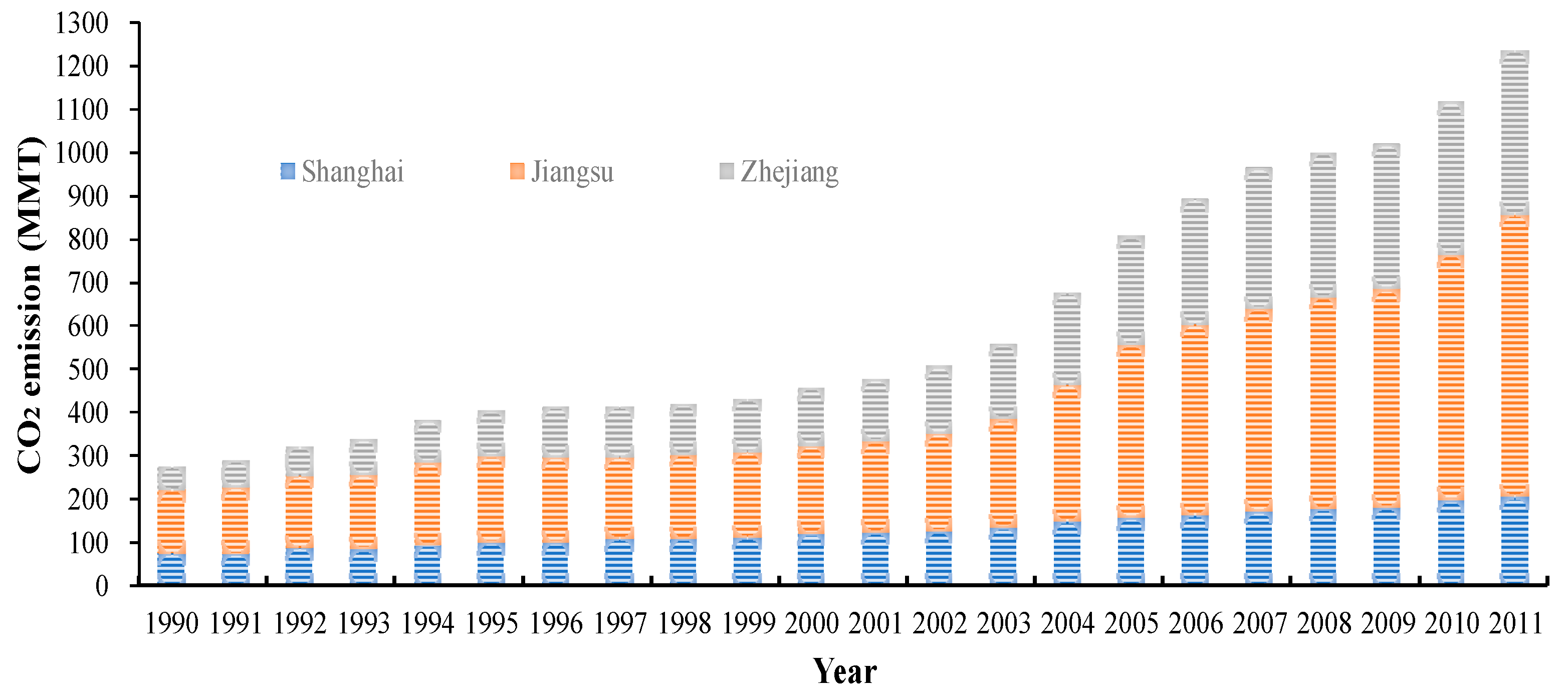
Technology level plays an important role in reducing CO₂ emissions in different ways such as increasing energy efficiency, improving economic structure, and developing decarbonization technology. Energy intensity, calculated as energy consumption per unit of GDP (taken the year of 2005 as the GDP base period), is one of the most frequently-used variables in the STRIPT model for measuring the technology level (Liu and Xiao, 2018) [46]. As illustrated in Figure 4, the overall trend of energy intensity in YRD was downward, decreasing from 1.71 tce/ten thousand CNY in 1990 to 0.69 tce/ten thousand CNY in 2011, at an average annual rate of 4.23 percent. The disparity in energy intensity between the three regions gradually diminished during the sample period.

3.2.5. CO₂ Emission

Many relevant studies adopt the variable of carbon dioxide per capita to describe the environmental pressure. Actually, in the IPAT model, I refers to total environmental pressure (Ehrlich and Holdren, 1971) [30]. Therefore, we employed total CO₂ emission as the explained variable. According to the actual situation of energy consumption in YRD, this study estimated CO₂ emission based on final energy consumption. Since YRD’s electricity and thermal power consumption are supplied by both domestic regions and outside neighboring cities, it is not appropriate to simply treat electricity and thermal power as final energy consumption for the calculation. Thus, in this empirical study, we only calculated the CO₂ emissions from domestic electricity and thermal power production by considering the fuel input during their production.

By referring to the China Energy Statistical Yearbook 1996–2012, 11 major fuels (raw coal, washed coal, coke, crude oil, gasoline, kerosene, diesel, fuel oil, LGP, refinery dry gas, and natural gas) were selected to calculate CO₂ emission by multiplying the consumption of each fuel with the carbon emission factor coefficient and the standard coal coefficient as follows:

$$G={\displaystyle \sum _{i=1}^{11}{G}_{ij}={\displaystyle \sum _{i=1}^{11}{E}_{ij}\times C_i\times F_i\times \frac{44}{12}}}$$

(7)

where G is the total CO₂ emissions in YRD, G_ij represents CO₂ emissions by the i^th fuel in j region, E_ij denotes the consumption of the i^th fuel in j region, C_i is the carbon emission factor coefficient of the i^th fuel, and F_i is the standard coal coefficient of the i^th fuel. The values of C_i and F_i are presented in

Table 1. Carbon emission factor and standard coal coefficient.

Fuel	Ci (t/tce)	Fi
Raw coal	0.7559	0.7143 kgce/kg
Washed coal	0.7559	0.9000 kgce/kg
Coke	0.8550	0.9714 kgce/kg
Crude oil,	0.5857	1.4286 kgce/kg
Gasoline	0.5538	1.4714 kgce/kg
Kerosene	0.5714	1.4714 kgce/kg
Diesel	0.5921	1.4571 kgce/kg
Fuel oil	0.6185	1.4286 kgce/kg
LPG	0.5024	1.7143 kgce/kg
Refinery dry gas	0.4602	1.5714 kgce/kg
Natural gas	0.4483	1.330 kgce/m3

Source: C_i comes from the IPCC National Greenhouse (2006). F_i comes from the China Energy Statistical Yearbook 2008.

.

YRD’s CO₂ emissions are presented in Figure 5. It indicates that the emissions continuously increased from 272.45 million metric tons (MMT) in 1990 to 1238.06 MMT in 2011 at an average annual growth rate of 7.47 percent. The growth rate from 2001–2011 was much higher than that from 1990–2000, and the corresponding rate gap was as much as 4.79 percent. Moreover, Figure 5 shows the obvious regional disparities of CO₂ emissions among Shanghai, Jiangsu, and Zhejiang, although they all showed an increasing trend. Specifically, the annual increase rate of CO₂ emissions in Shanghai was only 5.03 percent (the lowest) during the period over 1990 and 2011, while the annual increase rate of CO₂ emissions in Jiangsu and Zhejiang was as high as 7.37 and 9.92 percent (the highest), respectively.

4. Empirical Results

4.1. Unit Root Test

It is necessary to test the stationarity of time series before we conduct the cointegration analysis, in order to avoid some problems like spurious regression. One commonly-applied approach to do the unit root test is the augmented Dickey–Fuller (ADF) test. Usually, the ADF test can be described as Equation (8):

$$\Delta x_t=\alpha +\beta t+\delta x_{t-1}+{\displaystyle \sum _{j=1}^p{\lambda }_j}\Delta x_{t-j}+u_t$$

(8)

in which the subscript t is the t^th period, and t in Equation (8) is a time variable, representing a deterministic trend (if any) defined by t. Δx_t = x_t-x_t-1, where x is the first-order differencing variable, α is the constant term, u_t is the error term, and δ, β, and λ are all the regression coefficient.

In the ADF test, the null hypothesis is H₀: δ = 0, which represents that there are unit roots and series are nonstationary; the alternative hypothesis is H₁: δ < 0, which stands for that there are no unit roots and series are stable. The test results are shown in

Table 2. Results of the augmented Dickey–Fuller (ADF) test.

Series	ADF Statistics	Result	First Difference	ADF Statistics	Result
lnCARBON	0.50 (0.98 *)	nonstationary	D(lnCARBON)	−2.61 (0.047 *)	stationary
lnENERTEN	−1.19 (0.65 *)	nonstationary	D(lnENERTEN)	−3.31 (0.03 *)	stationary
lnPERGDP	−2.64 (0.1 *)	nonstationary	D(lnPERGDP)	−2.31 (0.049 *)	stationary
lnPOPULATION	2.0 (0.99 *)	nonstationary	D(lnPOPULATION)	−3.44 (0.02 *)	stationary
lnURBAN	−1.41 (0.55 *)	nonstationary	D(lnURBAN)	−5.03 (0.007 *)	stationary

* indicates the statistical significance at the level of 5%.

.

It turns out that all variables were nonstationary series, but were stable at a significance level of 5% with the first difference. Therefore, time series were considered stable after taking the first-order difference, which met the necessary conditions of constructing the cointegration model.

4.2. Johansen Co-Integration Test

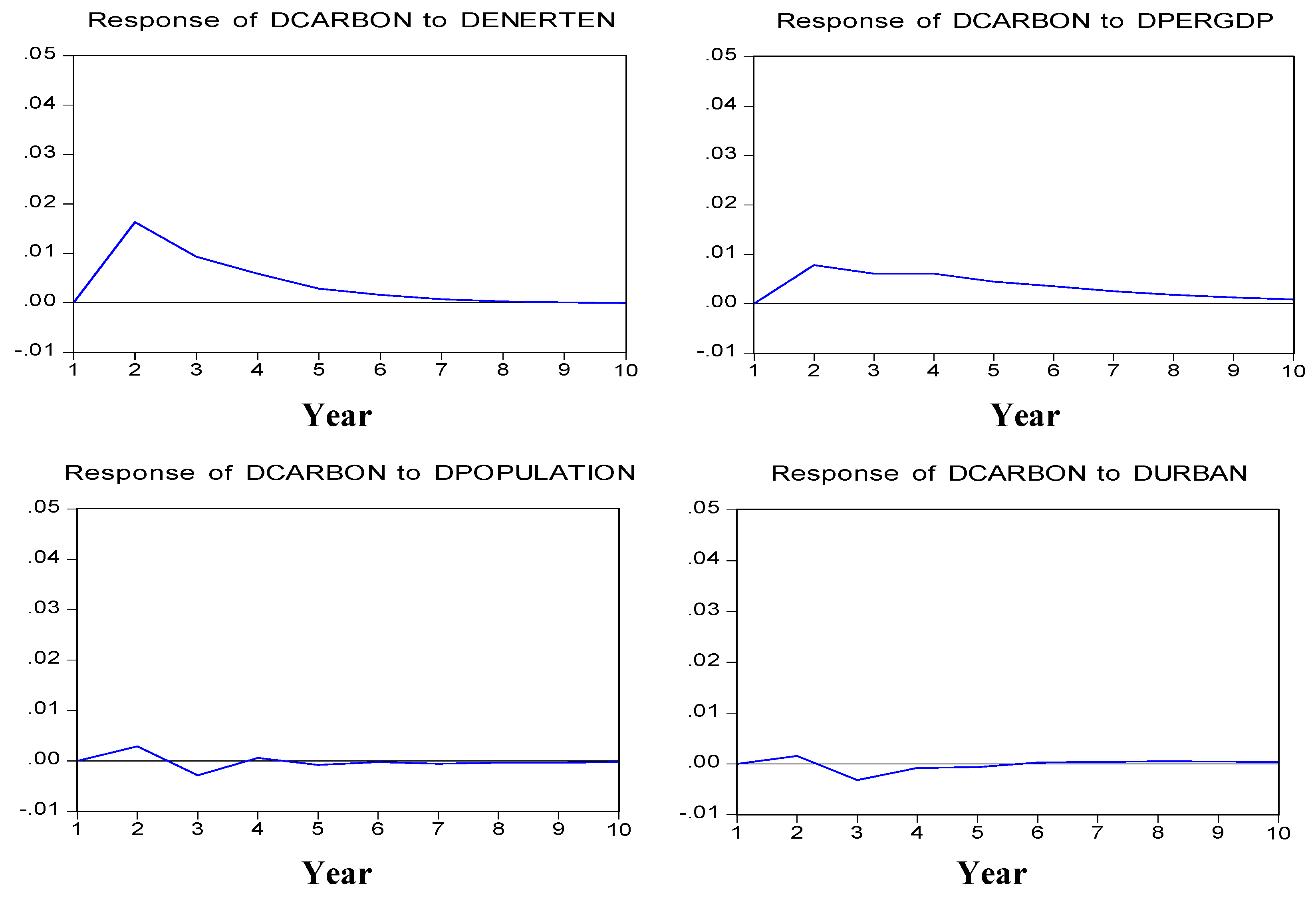
The validity of the regression analysis will be influenced if the time series is nonstationary. Co-integration theory indicates that stationarity may occur when two or more non-stationary time series are specially combined. Thus, equilibrium relations can be found among these nonstationary time series. The Engle–Granger test and Johansen cointegration test are frequently adopted methods to test the long-term equilibrium relationship. We chose the Johansen cointegration test to analyze the long-term equilibrium relationships between CO₂ emissions and the four variables described, because it is a multivariate cointegration method and can precisely determine the number of cointegration relationships through the trace statistic test. To save space, interested readers can refer to Johansen and Juselius (1990) [47] and Ouyang and Lin (2017) [45] for a detailed description.

Table 3. The results of the Johansen cointegration test.

Hypothesized No. of CE (s)	Eigenvalue	Trace Statistic	0.05 Critical Value	Prob. **
None *	0.981936	155.4233	69.81889	0.0000
At most one *	0.846057	75.14633	47.85613	0.0000
At most two *	0.617977	37.72283	29.79707	0.0050
At most three *	0.602754	18.47736	15.49471	0.0172
At moss four *	0.000668	0.013365	3.841466	0.9078

* represents the rejection of the hypothesis at the 0.05 level. ** MacKinnon–Haug–Michelis (1999) p-values.

shows the results of the Johansen cointegration test. According to the trace statistic test, there was four cointegrations among LNCARBON, LNENERTEN, LNPERGDP, LNPOPULATION, and LNURBAN since the trace statistics were greater than critical value at the 5% significance level. Thus, it can be confirmed that there exist long-term equilibrium relationships between CO₂ emission and energy intensity, economic development, population, and urbanization in the YRD.

Considering the standardized cointegration coefficients in the assumption of existing cointegration relations, we extracted a cointegration equation as follows:

$$\begin{gathered} \ln CARBON=2.5\ln ENERTE{N}_t+0.61\ln PERGD{P}_t+1.16\ln POPULATIO{N}_t+2.2\ln URBA{N}_t-14.59 \\ \begin{array}{cccc}\left(0.074\right)& \left(0.056\right)& \left(0.44\right)& \left(0.16\right)\\ \left[33.96\right]& \left[11.05\right]& \left[2.65\right]& \left[13.55\right]\end{array} \end{gathered}$$

(9)

Each number in the parentheses of Equation (9) represents the standard deviation of the explanatory variable above it, and each number in the square brackets of Equation (9) represents the t-statistic of the explanatory variable above it. All coefficients were positive, and this is in line with the economic interpretation, which means the increase of the four explanatory variables will result in the further increase of CO₂ emissions in YRD. Specifically, CO₂ emissions will respectively increase by 2.5%, 2.2%, 1.16%, and 0.6%, with a 1% increase in energy intensity, urbanization level, population, and GDP per capita.

4.3. IRF Results

To describe the duration of the impacts and the dynamic disturbance of whole system when one variable changes, IRF is employed in this section. Figure 6 depicts the results of IRF, which was carried out using a horizon of ten-year periods. The horizontal x-axis represents the duration period of the impacts (unit: year), and the vertical y-axis represents the impact magnitude of a shock. It can be seen that:

• One standard deviation shock in energy intensity will result in a sharp increase of CO₂ emissions, reaching its maximum in the second period. After that, CO₂ emissions ill decrease rapidly and finally stagnate after the eighth period.
• CO₂ emissions in YRD showed a positive response to GDP per capita both in the short and long term; however, the intensity of response reduced over time. The response trajectory was similar to the shock in energy intensity on CO₂ emissions. However, the duration of impact was longer than that from energy intensity. The CO₂ emissions level did not achieve stagnation before the tenth period.
• In response to shocks coming from the population, the CO₂ emissions increased in the first two periods and then decreased, with the reaction turning to a negative response in the third period, slightly fluctuating between the fourth period and fifth period, and eventually stagnating after that.
• The reaction of CO₂ emissions to shock in urbanization maintained a positive response state firstly and reached its maximum in the second period. Then, the response gradually decreased and reached its largest negative value at the end of the third period, then maintained a very small negative value between the fourth and fifth period and eventually stagnating.

It can be seen that all reactions eventually converged, indicating that the VAR system was stable and could improve the robustness of the estimation results.

4.4. VD Results

In order to further examine the relative importance of the four variables to CO₂ emissions in YRD, VD analysis was used. It decomposes the mean squared error of one endogenous variable into the contribution proportion of the shocks to all variables so as to understand the impact magnitude of these variables. The results are reported in

Table 4. Variance decomposition of CO₂ emissions.

Period	S.E.	CARBON (%)	ENERTEN (%)	PERGDP (%)	POPULATION (%)	URBAN (%)
1	0.048120	100.0000	0.000000	0.000000	0.000000	0.000000
2	0.056295	89.35247	7.132033	2.020358	0.132983	1.362158
3	0.059040	86.22024	9.546842	2.740183	0.179444	1.313292
4	0.060342	84.82223	10.11490	3.603223	0.190561	1.269086
5	0.060947	84.33591	10.18274	4.039191	0.193422	1.248743
6	0.061263	84.09282	10.14689	4.327790	0.194559	1.237940
7	0.061418	83.98242	10.10953	4.471183	0.204946	1.231927
8	0.061495	83.92371	10.08601	4.547782	0.212359	1.230137
9	0.061531	83.89404	10.07416	4.583483	0.219036	1.229288
10	0.061547	83.87862	10.06894	4.600212	0.223048	1.229182

and the variance decomposition for a ten-year period was chosen to reflect both the short- and long-term effects.

For CO₂ emissions in YRD, energy intensity shock contributes most to its variability. Its contribution rate was 7.13% in the second period and then grew rapidly in the first five forecast periods, reaching the maximum value of 10.18% in the fifth period. Then, the contribution rate decreased slightly and reached 10.07% in the tenth period and overall represented an inverted U-shaped curve.

GDP per capita shock was the second contributor. At the two-year forecasting horizon, it accounted for 2.02% of the forecast error variance and continuously increased to 4.6% at the ten-year horizon.

Urbanization ranked third in its relative importance. However, different from energy intensity and GDP per capita, its contribution rate to the variability of CO₂ emissions represented a slightly decreasing tread, from 1.36% in the short term to 1.23% in the long term.

Population had the least ability to explain the variability of CO₂ emissions. It could only explain 0.13% of the forecast error variance in the short term, while slightly increasing to 0.22% in the long term.

4.5. Prediction of CO₂ Emissions in YRD

4.5.1. Construction of the SVM Model

SVM is a method that can deal with small samples, nonlinearity, and high-dimensional pattern recognition. CO₂ emission time series in YRD are characterized by nonlinear processes, multiple influencing factors, and short historical data, as described in Section 3. Therefore, an SVM model will be constructed to predict YRD’s CO₂ emission level from 2015–2020 in this section. The specific procedure is as follows.

Step 1: Selecting the input and output variables. To ensure the uniformity and comparability of the research, the influencing factors were still based on the extended STIRPAT model described in the above sections. Then, CO₂ emissions in YRD from 1990–2011 and its influencing factors could be combined into a sample set (x_i⁰, y_i⁰), where x_i is the input and y_i is the output.

Step 2: Normalization of data. To eliminate the dimensional effects in the historical data, we carried out the normalization processing of all input and out variables as following, so that all the data were in the range of [0,1].

$${\mathrm{x}}_{ij}=\frac{x_{il}^0-\underset{i=1,2,\cdots ,n}{\min x_{ij}^0}}{\underset{i=1,2,\cdots ,n}{\max x_{ij}^0}-\underset{i=1,2,\cdots ,n}{\min x_{ij}^0}},i=1,2,\cdots ,n;j=1,2,3,4$$

(10)

$$y_i=\frac{y_i^0-\underset{i=1,2,\cdots ,n}{\min y_i^0}}{\underset{i=1,2,\cdots ,n}{\max y_i^0}-\underset{i=1,2,\cdots ,n}{\min y_i^0}},i=1,2,\cdots ,n$$

(11)

Step 3: Selecting the kernel function. Mapping low-dimensional vectors into a higher-dimensional space will increase the complexity of computing; therefore, the kernel function is needed, which is considered a good solution to this problem. Selecting the right kernel function is the key to SVM. It provides four basic kernel functions, and the radial basic function (RBF) is considered to be better because of its simplicity, reliability, and efficiency (Mladenović et al., 2016). Hence, in this study, the RBF was adopted.

Step 4: Determining training samples and parameter tuning. Before predicting the CO₂ emission level in 2020, it was necessary to test the validity of the SVM model. The test (learning) procedure had two steps: selecting the training sample out of the sample dataset and estimating the separating hyperplane based on this; evaluating the model’s performance in the left subset of the sample dataset. Based on the study of Papadimitriou et al. (2014) [48], 80–95% of the whole sample dataset was needed for evaluating the model’s performance. Therefore, we selected the historical data from 1990–2007 as the training sample to obtain the SVM model, and this model was used to forecast the CO₂ emissions from 2008–2011. Then, the effectiveness of the SVM model could be verified by comparing the predicted and actual values from 2008–2011.

During the training and predicting process, optimally choosing the SVM penalty parameter (C) and the RBF kernel function parameter ơ² was the key. The error of the prediction results was taken as the evaluation criterion, and the appropriate values of C and ơ² were determined according to the performance of the verification set. After repeated tests, we can see that when C = 5.8 and ơ² = 0.1, the prediction results were satisfactory.

Step 5: Constructing the SVM model. After the parameters were optimally chosen, YRD’s CO₂ emissions from 2015–2020 could be forecasted based on the SVM model.

4.5.2. Prediction Results of CO₂ Emissions

In order to improve the accuracy of forecasting, the future values of the four influencing factors in this paper were all defined based on the government policy.

Energy intensity by 2020: The Comprehensive Work for Conserving Energy and Reducing Emissions for the Twelfth Five-Year (2011–2015) Planning has explicitly set the goal that YRD’s energy intensity by 2015 should decrease by 18% compared with 2010. Further, the Comprehensive Work for Conserving Energy and Reducing Emissions for the Thirteenth Five-Year (2016–2020) Planning stated that, at the end of 2020, energy intensity should further decrease by 17% on the basis of 2015. This paper adopted the goals set by the two government documents as the benchmark scenario (0.49 tce/ten thousand CNY) and further set the value floating up and down 0.5%.

Urbanization rate by 2020: According to the Regional Planning for the Yangzi River Delta Region, the share of urban population in total will be up to 72% by 2020. This article adopted this goal by 2020 as the benchmark scenario (72%) and further set the value floating up and down 0.4%.

GDP per capita by 2020: The Regional Planning for the Yangzi River Delta Region clearly put forward the aim of YRD’s GDP per capita by 2020, that is 0.11 million CNY. This article adopted this goal as the benchmark scenario and further set the value floating up and down 0.5%.

Population by 2020: According to the 13^th Five-Year Planning for Population Development in Jiangsu and Zhejiang Province issued in 2017, the permanent population in the two provinces will reach about 82 million and 57.5 million by the end of 2020, respectively. As for Shanghai, the government tends to control population, and its National Economic and Social Development Outline for the Thirteenth Five-Year Planning clearly indicated that the permanent population in Shanghai should not exceed 25 million by 2020. This article adopted these goals as the benchmark scenario (164.5 million) of YRD’s population by 2020 and further set the value floating up and down 0.5%.

CO₂ emissions prediction: By applying the above future values of the influencing factors into the SVM model, we can get the predicted CO₂ emissions from 2015–2020 (baseline scenario), as shown in the second column of

Table 5. Prediction of the impact of influencing factors on CO₂ emissions in YRD under different situations (MMT).

Year	Baseline Scenario	Energy Intensity		Urbanization Level		Per Capita GDP		Population
		+0.5%	−0.5%	+0.4%	−0.4%	+0.5%	−0.5%	+0.4%	−0.4%
2015	1323.8	1324	1323.6	1325.3	1322.3	1325.9	1324	1328.8	1318.8
2016	1370.8	1370.9	1370.8	1372.3	1369.4	1372.9	1370.9	1375.5	1366
2017	1416	1416.1	1415.9	1417.4	1414.6	1418.1	1416.1	1420.4	1411.5
2018	1458.7	1458.8	1458.6	1460	1457.4	1460.7	1458.8	1462.8	1454.6
2019	1497.7	1497.7	1497.6	1498.9	1496.4	1499.5	1497.7	1501.3	1493.9
2020	1534.1	1534.2	1534.1	1535.3	1533	1535.7	1534.1	1537.3	1530.9

. The results were renormalized based on Equation (12):

$$\stackrel{\wedge }{y_s}f\left(x_s\right)\left(\underset{i=1,2,\cdots ,n}{\max y_i^0}-\underset{i=1,2,\cdots ,n}{\min y_i^0}\right)+\underset{i=1,2,\cdots ,n}{\min y_i^0}$$

(12)

The result showed that CO₂ emissions in YRD presented an observed increase from 2015 (1323.8 MMT) to 2020 (1534.1 MMT) under the baseline scenario, increasing by 37.2% compared with 2010. Moreover, CO₂ emissions increase compared to the baseline scenario, whichever influencing factor is fine-tuned upward, as shown in Columns 3–10 of Table 5. However, when the four variables were fine-tuned downward, the effects on CO₂ emissions were different. A 0.5% increase in energy intensity and per capita GDP had little impact on CO₂ emissions. In contrast, the downward fine-tuning on the urbanization rate and population caused an obvious decrease of CO₂ emission level. Whether it was fine-tuned upward or downward, the change impact of energy intensity on the baseline scenario was the smallest among the four factors, and the impact of population, in contrast, was the largest.

5. Discussion

5.1. The Overall Change in CO₂ Emission Level

From 1990–2011, CO₂ emission levels in YRD presented a continued growth trend. According to the prediction, CO₂ emissions will still increase by 2020. However, if we take ten years as an observation period, we can find that the growth rate of CO₂ emissions will show an inverted-U shape. The growth rate between 2000 and 2010 was as high as 145.89%, which was the highest among the three periods. By contrast, the growth rate from 2010–2020 was the lowest, which was only 37.2%, far below that of 1990–2000 (66.93%).

Figure 7 illustrates the growth rate change trending of CO₂ emissions from 1991–2011. It can be divided into five parts: a slowing increase of the growth rate from 1991–1994 (except 1993), followed by a sharp decrease in 1994–1997, then a significant increase in 1997–2004, followed by another obvious decline from 2004–2009, and then a slight increase in 2009–2011.

The reason for a lower growth rate of CO₂ emissions in 1994–1997 may be the relatively low growth rate of the economy. From 1994–1997, China implemented a moderately tight fiscal and monetary policy to tackle serious inflation. With these policies, the infrastructure investment slowed down, and so did the energy consumption, which in turn resulted in the low growth rate of CO₂ emissions. However, the outbreak of the Asian financial crisis in 1997 and the great flood in 1998 produced large shocks on the slowed domestic economy, which led the Chinese government to change the previous policies into pro-active fiscal and sound monetary policies. These stimulated the domestic market needs and accelerated the economic development, which in turn led to a huge increase in the growth rate of energy demand and the related CO₂ emissions. The reason for the decreasing growth rate in 2004–2009 in Figure 7 was similar to that of 1994–1997. The government implemented sound fiscal and monetary policies to tackle the inflation pressure and the increasing energy prices, which curbed the growth rate of CO₂ emissions. As for the increasing growth rate from 2009–2011 in Figure 7, the reason may lie in China’s four trillion CNY investment plan after the global financial crisis in 2008.

5.2. The Relationship between CO₂ Emission and Urbanization Rate

The correlation between urbanization rate and CO₂ emissions had a significant spatial heterogeneity (Yao et al., 2018; Xu and Lin, 2015; Al-mulali et al., 2012) [20,49,50]. This paper revealed the urbanization and CO₂ emissions had a positive correlation in YRD. However, its shock effect on CO₂ emissions was not significant, far below the energy intensity. This is consistent with the study of He et al. (2017) [51]. Further, the shock effect was positive only in the short term. After getting the highest value, the effect tended to decline and eventually became negative in the long term (see Figure 6). Moreover, its contribution rate also showed the decline trend in the long term (see Table 4). These results indicated that there may exist an inverted U-shaped relationship between urbanization and CO₂ emissions in YRD in the long term. This is consistent with the study of Shi and Li (2018) [12], which revealed that the relationship between urbanization rate and CO₂ emissions may become negative in China, when the urbanization rate reached the turning point (about 73%).

Structural transformation is considered to be a critical factor to understand the impact mechanism of urbanization on CO₂ emissions (Madlener and Sunak, 2011) [13], and the reason for high carbon emissions in Chinese cities mainly lies in the industrial sector. This study calculated CO₂ emissions of YRD’s industrial sector from 1995–2011 based on Equation (7) and found that this sector accounted for over 80% of total CO₂ emissions in each year. This indicates that the initial stage of urbanization in YRD required large investment in infrastructure and mainly depended on high energy-consuming manufacturing. Therefore, related CO₂ emissions increased with the increase of the urbanization rate. Just as shown in Figure 8, the annual growth rate of CO₂ emissions from the industrial sector increased from 1.3% in 1996 to 25.7% in 2004, during which the urbanization rate increased from 37.14–53.5% (see Figure 2). However, with the acceleration of the urbanization process, the increasing rate of CO₂ emissions from the industrial sector decreased gradually, as shown in Figure 8. This may be due to the low-carbon technology development and the transfer of energy-consuming industries to other regions during the urbanization process. These results are consistent with the study of Shi and Li (2018) [12], which pointed out that in the provinces where the urbanization rate and the proportion of service sector were both high, such as Shanghai, Jiangsu, and Zhejiang, the carbon emissions increased with the acceleration of the urbanization process at the beginning; however, the increasing rate of carbon emission will gradually decrease after the urbanization rate reaches a relative high point.

5.3. The Relationship between CO₂ Emission and Energy Intensity

The change of economic structure and the development of low-carbon technology can influence energy intensity and thus exert an effect on CO₂ emissions. This paper revealed that the impact of energy intensity on YRD’s CO₂ emissions was the greatest among all the influencing factors (see Figure 6 and Table 4). According to the IRF research, the maximum value of the energy intensity’s shock effect was the highest compared to other factors. The shock effect remained positive both in the short and long term. The contribution rate of energy intensity to the change of CO₂ emissions was over 10%, both in the short and long term, which was also the largest compared to other factors (see Table 4). According to the study of Wang and Zhao (2015) [52] and Shi and Li (2018) [12], the effect of energy efficiency largely depended on the economic development and urbanization level. YRD, the fastest growing economy with a high urbanization level, has an advanced technical level and high-tech industries, which can greatly improve energy efficiency and reduce energy-related CO₂ emissions. In addition, the economic structure is gradually changing, and the tertiary industry increased from 33.4% in 1995 to 45.9% in 2011, which would significantly improve the energy intensity and reduce the related CO₂ emissions.

However, after getting the highest value, the shock effect began to decline in the long term (see Figure 6); so did the contribution rate, which became relatively stable in the long term (see Table 4). This situation represents an inverted U-shaped curve and implies that the decreasing effect of energy intensity may become relatively smaller in the long term. The small change of the simulation results under different scenarios also verified the result (See Table 5). Some reasons can explain this. According to the study of Lin and Zhu (2017), the industrial structure is an important factor influencing energy intensity; however, the influence tends to be stable in the long term. This means the room for improvement of YRD’s industrial structure was relative smaller in the long term, which in turn influenced the continuous improvement of energy intensity. In addition, the impact of energy intensity on CO₂ emissions may become relatively stable once the energy structure achieves fundamental transformation in the long term. The energy rebound effect may also restrain the decreasing effect, since lower energy prices and extensive economic growth caused by improvement in energy efficiency will in turn stimulate more energy consumption [45]. According to the study of Ouyang et al. (2018) [45], the direct energy rebound of the YRD’s industrial sectors is approximately 40.04%.

5.4. The Relationship between CO₂ Emission and GDP per Capita

It seems that most literature studies agree that GDP per capita has a positive influence on CO₂ emissions, and this paper also demonstrated this. However, the studies differed in the magnitude of this effect due to the regional difference. This paper showed the dynamic impact of GDP per capita ranked the second among all the influencing factors, relatively smaller than energy intensity (see Table 4). In contrast, the shock effect of GDP per capita on CO₂ emissions lasted longer than all other factors (See Figure 6). Moreover, the contribution rate of GDP per capita had the fastest growth rate, increasing from 2.02 in the second period to 4.6 in the tenth period (see Table 4). The fine-tuning of GDP per capita also had surprising and interesting results. Upward fine-tuning can obviously increase the CO₂ emissions; however, downward fine-tuning had almost no impact on CO₂ emissions. These all demonstrate that the fast growth of the economy in YRD was still accompanied by increasing CO₂ emissions, and the turning point of the Kuznets curve has not yet appeared. The finding supports the results obtained by Alam et al. (2016) [53].

5.5. The Relationship between CO₂ Emission and Population Size

It is generally recognized that population size is an influencing factor for CO₂ emissions. This paper also revealed that total population had a positive influence on YRD’s CO₂ emissions. As for the magnitude of influence, however, its contribution was not significant. According to the results of variance decomposition, the contribution rate of the total population to CO₂ emissions was the least compared to other factors, both in the short and long term. This finding is consistent with the studies of Song et al. (2015) [28] regarding that population plays a negligible role in YRD’s CO₂ emissions compared to economy scale and energy intensity. Wang and Zhao (2015) [52] also presented that the effect of population on CO₂ emissions is smallest in China’s developed regions and largest in developing regions. The main reason might lie in the slow growth of population in YRD, which may restrain its influencing force on CO₂ emissions (Song et al., 2015) [28]. YRD, one of the most developed regions in China, has a relatively higher cost of living and stricter population control measures compared to the developing regions, which may influence the population inflow. In contrast, the developing regions have a faster economic growth than the under developed ones and a lower living cost than the developed ones, which make them more attractive for many people.

6. Conclusions

• Johansen cointegration test results provided evidence of the existence of the cointegration relationship among urbanization, population, economy growth, energy intensity, and CO₂ emissions.
• During the urbanization process, YRD’s CO₂ emissions continued increasing and was predicated to further increase in the long term. However, the contribution of urbanization to emissions continued to decline in the long term. The dynamic shock of urbanization on emissions in the long term even changed to negative. These findings mean that there may exist an inverted U-shaped relationship between urbanization and CO₂ emissions when the turning point comes. Therefore, there is no need for YRD’s government to sacrifice the urbanization process for emission reduction. This is different from the suggestion that China should slow down the process of urbanization in order to combat CO₂ emission (Zhang and Lin, 2012) [7].
• All the model results indicated that energy intensity had the greatest impact on YRD’s CO₂ emissions. Therefore, increasing low-carbon technology levels and lowering energy intensity is still the main task of the transition to a low-carbon economy in YRD. First, the efficiency of energy utilization should be enhanced. YRD can fully take advantage of high-level foreign investment itself to accelerate the introduction, digestion, and absorption of advanced low-carbon technologies, establish bilateral or multilateral energy efficiency cooperation plans, and promote the improvement of energy efficiency. Second, the energy structure should be further adjusted by increasing the proportion of non-fossil energy consumption. The coal consumption should be controlled, and economic and effective clean coal technologies should be applied. Moreover, clean and renewable energy sources, such as wind, solar, biomass, geothermal, and water, should be vigorously developed. The governments should actively promote the construction of nuclear energy in Zhejiang and Jiangsu.
• The contribution of GDP per capita to CO₂ emissions is higher than the population and urbanization rate. However, the finding related to GDP per capita, which needs to be emphasized most, is its fastest growth rate contribution. This indicates that the economic development in YRD is always accompanied by large emissions, and this trend is predicted to last in the future. The Kuznets curve does not exist in the current YRD.
• The results showed that population contributed the least to YRD’s CO₂ emissions, far below the three other factors, and the impact was negligible. This means that the policies related to population control in YRD can hardly achieve emission reductions.

References

1. Al-Mulali, U.; Fereidouni, H.G.; Lee, J.Y.M.; Sab, C.N.B.C. Exploring the relationship between urbanization, energy consumption, and CO2 emission in MENA countries. Renew. Sustain. Energy Rev. 2015, 23, 107–112. [Google Scholar] [CrossRef]
2. Chikaraishi, M.; Fujiwara, A.; Kaneko, S.; Poumanyvong, P.; Komatsu, S.; Kalugin, A. The moderating effects of urbanization on carbon dioxide emissions: A latent class modeling approach. Technol. Forecast. Soc. Chang. 2015, 90, 302–317. [Google Scholar] [CrossRef]
3. International Energy Agency. World Energy Outlook; IEA: Paris, France, 2008. [Google Scholar]
4. National Bureau of Statistics of China. China Statistical Yearbook 2018; China Statistics Press: Beijing, China, 2018.
5. Gregg, J.S.; Andres, R.J.; Marland, G. China: Emissions pattern of the world leader in CO2 emissions from fossil fuel consumption and cement production. Geophys. Res. Lett. 2008, 35, 135–157. [Google Scholar] [CrossRef]
6. Shen, L.; Cheng, S.; Gunson, A.J.; Wan, H. Urbanization, sustainability and the utilization of energy and mineral resources in China. Cities 2005, 22, 287–302. [Google Scholar] [CrossRef]
7. Zhang, C.; Lin, Y. Panel estimation for urbanization, energy consumption and CO2 emissions: A regional analysis in China. Energy Policy 2012, 49, 488–498. [Google Scholar] [CrossRef]
8. Lin, S.; Wang, S.; Marinova, D.; Zhao, D.; Hong, J. Impacts of urbanization and real economic development on CO2 emissions in non-high income countries: Empirical research based on the extended STIRPAT model. J. Clean. Prod. 2017, 166, 952–966. [Google Scholar] [CrossRef]
9. National Bureau of Statistics of China. China Energy Statistics Yearbook 2018; China Statistics Press: Beijing, China, 2018.
10. Bekhet, H.A.; Othman, N.S. Impact of urbanization growth on Malaysia CO2 emissions: Evidence from the dynamic relationship. J. Clean. Prod. 2017, 154, 374–388. [Google Scholar] [CrossRef]
11. Martinez-Zarzoso, I.; Maruotti, A. The impact of urbanization on CO2 emissions: Evidence from developing countries. Ecol. Econ. 2011, 70, 1344–1353. [Google Scholar] [CrossRef]
12. Shi, X.; Li, X. Research on three-stage dynamic relationship between carbon emission and urbanization rate in different city groups. Ecol. Indic. 2018, 91, 195–202. [Google Scholar] [CrossRef]
13. Madlener, R.; Sunak, Y. Impacts of urbanization on urban structures and energy demand: What can we learn for urban energy planning and urbanization management? Sustain. Cities Soc. 2011, 1, 45–53. [Google Scholar] [CrossRef]
14. Yang, Y.; Zhao, T.; Wang, Y.; Shi, Z. Research on impacts of population-related factors on carbon emissions in Beijing from 1984 to 2012. Environ. Impact Assess. Rev. 2015, 55, 45–53. [Google Scholar] [CrossRef]
15. Wang, Z.; Cui, C.; Peng, S. How do urbanization and consumption patterns affect carbon emissions in China? A decomposition analysis. J. Clean. Prod. 2019, 211, 1201–1208. [Google Scholar] [CrossRef]
16. Azizalrahman, H.; Hasyimi, V. A model for urban sector drivers of carbon emissions. Sustain. Cities Soc. 2019, 44, 46–55. [Google Scholar] [CrossRef]
17. Wang, Y.; Li, L.; Kubota, J.; Han, R.; Zhu, X.; Lu, G. Does urbanization lead to more carbon emission? Evidence from a panel of BRICS countries. Appl. Energy 2016, 168, 375–380. [Google Scholar] [CrossRef]
18. Sharma, S.S. Determinants of carbon dioxide emissions: Empirical evidence from 69 countries. Appl. Energy 2011, 88, 376–382. [Google Scholar] [CrossRef]
19. Zhang, N.; Yu, K.; Chen, Z. How does urbanization affect carbon dioxide emissions? A cross-country panel data analysis. Energy Policy 2017, 107, 678–687. [Google Scholar] [CrossRef]
20. Yao, X.; Kou, D.; Shao, S.; Li, X.; Wang, W.; Zhang, C. Can urbanization process and carbon emission abatement be harmonious? New evidence from China. Environ. Impact Assess. Rev. 2018, 71, 70–83. [Google Scholar] [CrossRef]
21. Zhu, H.-M.; You, W.-H.; Zeng, Z.-F. Urbanization and CO2 emissions: A semi-parametric panel data analysis. Econ. Lett. 2012, 117, 848–850. [Google Scholar] [CrossRef]
22. Shahbaz, M.; Chaudhary, A.; Ozturk, I. Does urbanization cause increasing energy demand in Pakistan? Empirical evidence from STIRPAT model. Energy 2017, 122, 83–93. [Google Scholar] [CrossRef] [Green Version]
23. Sheng, P.; Guo, X. The Long-run and Short-run Impacts of Urbanization on Carbon Dioxide Emissions. Econ. Model. 2016, 53, 208–215. [Google Scholar] [CrossRef]
24. Wu, Y.; Shen, J.; Zhang, X.; Skitmore, M.; Lu, W. Reprint of: The impact of urbanization on carbon emissions in developing countries: A Chinese study based on the U-Kaya method. J. Clean. Prod. 2017, 163, S284–S298. [Google Scholar] [CrossRef]
25. Yang, L.; Xia, H.; Zhang, X.; Yuan, S. What matters for carbon emissions in regional sectors? A China study of extended STIRPAT model. J. Clean. Prod. 2018, 180, 595–602. [Google Scholar] [CrossRef]
26. Ouyang, X.; Gao, B.; Du, K.; Du, G. Industrial sectors’ energy rebound effect: An empirical study of Yangtze River Delta urban agglomeration. Energy 2018, 145, 408–416. [Google Scholar] [CrossRef]
27. Li, J.; Huang, X.; Kwan, M.-P.; Yang, H.; Chuai, X. The effect of urbanization on carbon dioxide emissions efficiency in the Yangtze River Delta, China. J. Clean. Prod. 2018, 188, 38–48. [Google Scholar] [CrossRef]
28. Song, M.; Guo, X.; Wu, K.; Wang, G. Driving effect analysis of energy-consumption carbon emissions in the Yangtze River Delta region. J. Clean. Prod. 2015, 103, 620–628. [Google Scholar] [CrossRef]
29. Zhu, X.-H.; Zou, J.-W.; Feng, C. Analysis of industrial energy-related CO2 emissions and the reduction potential of cities in the Yangtze River Delta region. J. Clean. Prod. 2017, 168, 791–802. [Google Scholar] [CrossRef]
30. Ehrlich, P.R.; Holdren, J.P. Impact of population growth. Science 1971, 171, 1212–1217. [Google Scholar] [CrossRef]
31. Dietz, T.; Rosa, E.A. Effects of population and affluence on CO2 emissions. Proc. Natl. Acad. Sci. USA 1997, 94, 175–179. [Google Scholar] [CrossRef]
32. York, R.; Rosa, E.A.; Dietz, T. STIRPAT, IPAT and ImPACT: Analytic tools for unpacking the driving forces of environmental impacts. Ecol. Econ. 2003, 46, 351–365. [Google Scholar] [CrossRef]
33. Sims, C.A. Macroeconomics and Reality. Econometrica 1980, 48, 1–48. [Google Scholar] [CrossRef]
34. Hao, Y.; Wang, L.; Zhu, L.; Ye, M. The dynamic relationship between energy consumption, investment and economic growth in China’s rural area: New evidence based on provincial panel data. Energy 2018, 154, 374–382. [Google Scholar] [CrossRef]
35. Talbi, B. CO2 emissions reduction in road transport sector in Tunisia. Renew. Sustain. Energy Rev. 2017, 69, 232–238. [Google Scholar] [CrossRef]
36. Zhang, C.; Zhou, K.; Yang, S.; Shao, Z. Exploring the transformation and upgrading of China’s economy using electricity consumption data: A VAR–VEC based model. Phys. A Stat. Mech. Appl. 2017, 473, 144–155. [Google Scholar] [CrossRef]
37. Olson, E.; Vivian, A.J.; Wohar, M.E. The relationship between energy and equity markets: Evidence from volatility impulse response functions. Energy Econ. 2014, 43, 297–305. [Google Scholar] [CrossRef] [Green Version]
38. Wang, S.; Wang, J.; Zhou, Y. Estimating the effects of socioeconomic structure on CO2 emissions in China using an econometric analysis framework. Struct. Chang. Econ. Dyn. 2018, 47, 18–27. [Google Scholar] [CrossRef]
39. Cortes, C.; Vapnik, V. Support-Vector Networks. Mach. Learn. 1995, 20, 273–297. [Google Scholar] [CrossRef]
40. Wang, X.; Luo, D.; Zhao, X.; Sun, Z. Estimates of energy consumption in China using a self-adaptive multi-verse optimizer-based support vector machine with rolling cross-validation. Energy 2018, 152, 539–548. [Google Scholar] [CrossRef]
41. Mladenović, I.; Sokolov-Mladenović, S.; Milovančević, M.; Marković, D.; Simeunović, N. Management and estimation of thermal comfort, carbon dioxide emission and economic growth by support vector machine. Renew. Sustain. Energy Rev. 2016, 64, 466–476. [Google Scholar] [CrossRef]
42. Li, C.; Lin, S.; Xu, F.; Liu, D.; Liu, J. Short-term wind power prediction based on data mining technology and improved support vector machine method: A case study in Northwest China. J. Clean. Prod. 2018, 205, 909–922. [Google Scholar] [CrossRef]
43. Shi, A. The impact of population pressure on global carbon dioxide emissions, 1975–1996: Evidence from pooled cross-country data. Ecol. Econ. 2003, 44, 29–42. [Google Scholar] [CrossRef]
44. Cole, M.A.; Neumayer, E. Examining the Impact of Demographic Factors on Air Pollution. Popul. Environ. 2004, 26, 5–21. [Google Scholar] [CrossRef] [Green Version]
45. Ouyang, X.; Lin, B. Carbon dioxide (CO2) emissions during urbanization: A comparative study between China and Japan. J. Clean. Prod. 2017, 143, 356–368. [Google Scholar] [CrossRef]
46. Liu, D.; Xiao, B. Can China achieve its carbon emission peaking? A scenario analysis based on STIRPAT and system dynamics model. Ecol. Indic. 2018, 93, 647–657. [Google Scholar] [CrossRef]
47. Johansen, S.; Juselius, K. Maximum likelihood estimation and inference on co-integration. Oxf. Bull. Econ. Stat. 1990, 52, 169–201. [Google Scholar] [CrossRef]
48. Papadimitriou, T.; Gogas, P.; Stathakis, E. Forecasting energy markets using support vector machines. Energy Econ. 2014, 44, 135–142. [Google Scholar] [CrossRef]
49. Xu, B.; Lin, B. How industrialization and urbanization process impacts on CO2 emissions in China: Evidence from nonparametric additive regression models. Energy Econ. 2015, 48, 188–202. [Google Scholar] [CrossRef]
50. Al-Mulali, U.; Sab, C.N.B.C.; Fereidouni, H.G. Exploring the bi-directional long run relationship between urbanization, energy consumption, and carbon dioxide emission. Energy 2012, 46, 156–167. [Google Scholar] [CrossRef]
51. He, Z.; Xu, S.; Shen, W.; Long, R.; Chen, H. Impact of urbanization on energy related CO2 emission at different development levels: Regional difference in China based on panel estimation. J. Clean. Prod. 2017, 140, 1719–1730. [Google Scholar] [CrossRef]
52. Wang, Y.; Zhao, T. Impacts of energy-related CO2 emissions: Evidence from under developed, developing and highly developed regions in China. Ecol. Indic. 2015, 50, 186–195. [Google Scholar] [CrossRef]
53. Alam, M.M.; Murad, M.W.; Noman, A.H.M.; Ozturk, I. Relationships among carbon emissions, economic growth, energy consumption and population growth: Testing Environmental Kuznets Curve hypothesis for Brazil, China, India and Indonesia. Ecol. Indic. 2016, 70, 466–479. [Google Scholar] [CrossRef]
Figure 1. Population size of Yangtze River Delta (YRD) from 1990–2011.
Sustainability 11 04183 g001
Figure 2. Urbanization process of YRD from 1990–2011.
Sustainability 11 04183 g002
Figure 3. GDP per capita in YRD from 1990–2011.
Sustainability 11 04183 g003
Figure 4. Energy intensity trend of YRD from 1990–2011. Note: tce means ton of coal equivalent.
Sustainability 11 04183 g004
Figure 5. CO2 emission of YRD from 1990–2011.
Sustainability 11 04183 g005
Figure 6. Response of CO2 emission to the influencing variables in YRD.
Sustainability 11 04183 g006
Figure 7. Growth rate of CO2 emission.
Sustainability 11 04183 g007
Figure 8. Growth rate of CO2 emission from the YRD’s industrial sector.
Sustainability 11 04183 g008