Principal Component Analysis of the Potential for Increased Rail Competitiveness in East-Central Europe

Abstract

Increased rail competitiveness has been the objective of many countries around the world, including member states of the EU. Although railway market liberalization has always been accompanied by high expectations of increased efficiency and competitiveness, the overall impact of such decisions can be considered controversial. This paper aims to contribute to the scientific debate by conducting a factor analysis of some East-Central European countries from the aspect of rail freight competitiveness. Since many highly correlated factors influence competitiveness, its mathematical–statistical representation and analysis is difficult due to the high number of dimensions of the factor space. Moreover, competitiveness cannot be measured directly only as a latent variable which is a feature of Principal Component Analysis (PCA). The introduced PCA, model by way of reducing the number of dimensions, can highlight the relations among the attributes and determine the most crucial issues capable of increasing rail competitiveness in the given countries and also of clustering those national railway markets. Recommendations for structural changes in national rail freight markets of the region are also supplied. Our results show that international rail competitiveness depends rather on market efficiency than on market liberalization due to the fact that the Global Competitiveness Index and Export/Import attributes did not significantly correlate with market concentration. As for the larger domestic rail freight sectors, small freight forwarders—spawned by liberalization—are shown to play a significant role in increasing competitiveness.

1. Introduction

Economic theory states that market liberalization generally increases competition, hence motivates companies to more efficient and more productive operations that cause improved competitiveness in the market [1]. Regarding the European rail freight markets, the experience so far has not completely validated this logic of the theory [2]. On the one hand, several scientific studies confirm that the rail companies with the highest degree of independence from external influences are the most efficient and competitive players in the market [3]. Moreover, the expansion of the markets is often followed by increased technical innovation [4], which also contributes to efficiency. (In this paper, we use the term “competitiveness” in a broader sense than market efficiency. In our view, the notion of competitiveness covers both the efficiency/productivity of the operations and the demand for rail transport services. We also note that, in our paper, we only consider rail freight markets in our database and results. Although passenger rail markets undoubtedly have common characteristics with the rail freight sector such as infrastructure used and some macroeconomic attributes, there are a number of rail freight-specific ones as well. Nevertheless, in our literature review, we apply the most relevant references from findings related to the passenger rail market taking into account the differences.) Many researchers also state [5,6] that liberalization resulted in more efficient railway undertakings and higher consumer surplus. On the other hand, there are noteworthy studies that doubt the strong correlation between productivity and market liberalization in the railway industry. One of the best examples is the work of Bougna and Crozet [7], in which the authors applied an input–output approach to measure the productivity of 17 European railway systems with the dataset of Eurostat from 1997 to 2011. In terms of methodology, they used stochastic distance functions to measure productive efficiency and change, and subsequently a limited dependent variable model to test the impact of liberalization on productivity. Their conclusion was that, in Europe, policy makers should give priority to raising productivity instead of forcing market liberalization by all means.

Our paper aims to contribute to this debate by focusing on East-Central European rail freight markets, having been more recently liberalized than their western counterparts within the EU but already having accumulated an experience of over a decade of free market operation. The outcome so far has not been an unqualified success story in this region. Based on recent statistics, these liberalized rail freight markets have been stagnating for the past ten years [8]. Despite the availability of new business opportunities, nowadays, the rail freight sector of the region still suffers from low attractivity and capability [9] compared to other regions in Europe. Thus, analyzing examples of this east-central cluster of EU member states may suffice to draw some conclusions contributing to the ongoing debate on the real impacts of rail freight market liberalization.

For our analysis, first the proper indicators of productivity, efficiency and competitiveness need to be selected. Our objective was not only a comparison of the markets, but also their assessment from a competitiveness point of view considering the fact that pure transport volume data (export, import, transit) did not seem sufficient. The determination of the relevant attributes was partly based on the paper of Feuerstein, Busacker and Xu [10]. They examined 34 factors in five categories: technical, economic, social, political/legal and other. All factors were influencers of the open access competition in European long-distance passenger rail transport. (In our case, only freight service is examined but most of the factors are identical to that of passenger transport.) Among the 34 influencers of competition, the economic and political/legal clusters proved to be of highest importance; especially factors like market potential, access to attractive train paths and governments’ attitude were among the most important ones. The authors also stated that, for different countries, different influencing attributes proved to be important. Although they applied rather different influencers from ours, the study inspired us to perform our own analysis on rail freight competition and liberalization. Since, due to their methodology, they incorporated many intangible attributes in their calculation, instead we decided to use tangible datasets or reliable indices computed based on trustworthy sources and methodology.

Thus, to ensure arrival at appropriate findings, a relevant, reliable database and a suitable analytical tool are also required. The sources of our raw data are referenced in

Table 1. Sources of data.

Influencer Number	Source
1, 12, (9 calculated)	The Czech Republic, Slovakia: The Railway Infrastructure Administration, state organization https://www.szdc.cz/en/o-nas/zeleznice-cr.html Románia: Compartiment Mass Media, Relatii cu Publicul CFR Marfa s.a. http://www.cfrmarfa.cfr.ro/index.php?option=com_content&view=article&id=223&Itemid=69&lang=en Poland: PKP Polskie Linie Kolejowe S.A. https://en.plk-sa.pl/for-customers-and-partners/the-rules-for-allocating-train-paths/network-statement-20192020/ Hungary: Innovációs és Technológiai Minisztérium Nemzeti Közlekedési Hatóság vasúti főosztály adatszolgáltatások: https://www.nkh.gov.hu/web/vasuti-foosztaly1/a-szervezet
2, 3, 7, 8, 13, 15	Eurostat: Goods transported by type of transport (2004–2016) http://appsso.eurostat.ec.europa.eu/nui/show.do?dataset=rail_go_typeall&lang=en
4, 5, 6	Word Economic Forum: The Global Competitiveness Report: https://www.weforum.org/reports/the-global-competitiveness-report-2017–2018
14	Best available data: Czech: Network Statement: https://www.szdc.cz/web/en/our-railway/how-to-operate-on-our-railway/prohlaseni-2019, Slovakia: Železnice Slovenskej republiky Network Statement, 2007–2015 https://www.zsr.sk/dopravcovia/infrastruktura/podmienky-pouzivania-zel-infrastruktury/network-statement-2020-english-version/ Hungary: Network Statement 2007–2015 https://www2.vpe.hu/halozati-uzletszabalyzat-husz/hatalyos-husz-2007–2015, Polen: pkp polskie linie kolejowe s.a. network statement 2007–2015 https://www.plk-sa.pl/dla-klientow-i-kontrahentow/warunki-udostepniania-infrastruktury-i-regulaminy/regulamin-sieci/archiwum-regulaminow/ Romania: Network Statement 2007–2015, http://www.cfr.ro/index.php/ct-menu-item-126 Eurostat, https://eur-lex.europa.eu/LexUriServ/LexUriServ.do?uri=COM:2019:0051:FIN:HU:PDF
10	Railway enterprises—by type of enterprise [rail_ec_ent] Last update: 26 February 2018 www. http://appsso.eurostat.ec.europa.eu/nui/show.do?dataset=rail_ec_ent&lang=en

. The Herfindahl–Hirsch index (HHI) values were calculated from publicly available governmental publications.

In terms of methodology, a multivariate factor analysis technique, the Principal Component Analysis (PCA), was selected due to its capability of determining not only complex interactions of factors but also the clusterization of the entities while highlighting dependencies from background variables. In a 15-dimensional space, the Eucledian distance of the attributes cannot be determined, so the cluster analysis of the raw data is impossible. We used an 8-year dataset to examine five East-Central European (ECE) countries including Slovakia, the Czech Republic, Hungary, Poland and Romania, representing altogether 40 entities, which all have 15 coordinates due to the selected 15 attributes, which are rather difficult to handle with the general multivariate statistical techniques. Our basic research objective was the analysis of recently transitioned countries after their railway market liberalization, so the extension of the 40 entities was impossible due to obvious reasons (the rail freight markets of these countries were opened up in the last decade, so the time frame could not be extended neither could the number of examined countries). As a substantial reduction in the number of dimensions could significantly contribute to the efficacy of the analysis, PCA was selected as a useful methodological tool to that end. Furthermore, the research concept of analyzing the complex issue of competitiveness necessitated the assumption of “latent attributes” besides the provided 15 measured attributes. The method can be applied to various kinds of datasets not only to subjective, preference-based ones but also to “objective”, measurement-based datasets [11]. Additionally, one of PCA’s main areas of application is macroeconomics [12] and our dataset contained dominantly macroeconomic data.

In the following sections, firstly, we give an overview the existing literature references to the selected competitiveness attributes. Afterwards, the applied PCA methodology is introduced, followed by the results of the analyzed five countries. Finally, conclusions are drawn with outlined limitations and recommendations for further research.

2. Theory/Literature Overview on Competitiveness Factors of Rail Freight Markets

In order to apply a complex approach integrating technical, cost- and user-preference elements, we consider competitiveness as a combination of efficiency attributes and the demand for railway transport services. Demand is considered here as motivation for rail freight service and not as a consequence [13]. In the transportation literature, technical and cost issues are generally examined by statistical techniques [14] while, for preference analyses, multi-criteria decision-making techniques are applied [15]. In our study, influencing factors from both groups were selected and also direct competitiveness indices (Global Competitiveness Index (GCI), GCI6P, GCI2P) have been integrated to elaborate the dependencies of these influencers. Since it has been argued that single measures of competitiveness are not sufficient, several authors propose composite indices [16,17]. One of our objectives was to shed light on the connections of single factors and these composite indices—especially the Global Competitiveness Index (GCI)—in our paper.

Undoubtedly, one of the most important determining factors of rail freight and passenger transport competitiveness is the quality of the infrastructure. This assertion has been proven for passenger transport [18] and for freight [19,20,21]. In their exhaustive survey, Purwanto et al. [17] concluded that increased competitiveness is among the wider benefits of transport infrastructure investments. The second pillar of the GCI is also related to the quality of rail infrastructure of the national railway.

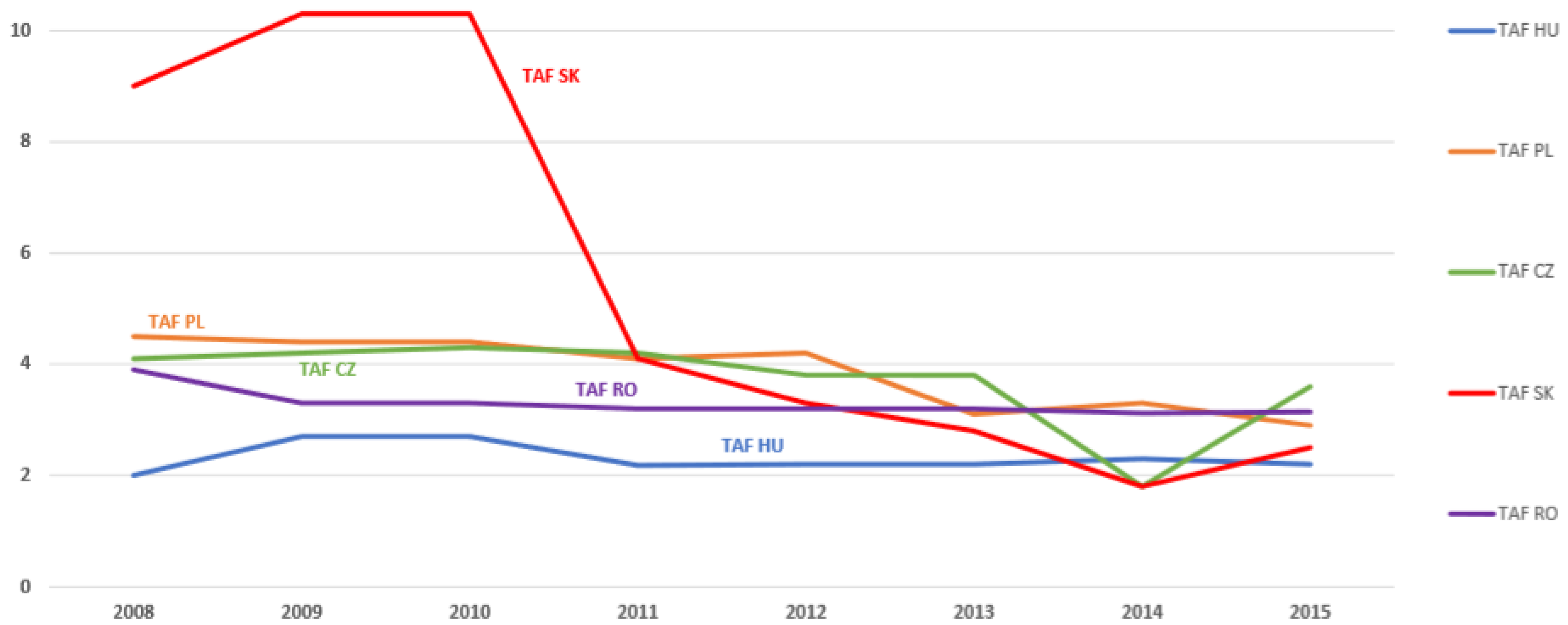
Rail freight market competitiveness and track access fees of the country or region also have interrelations [22], hence we applied this factor among the influencers in our model.

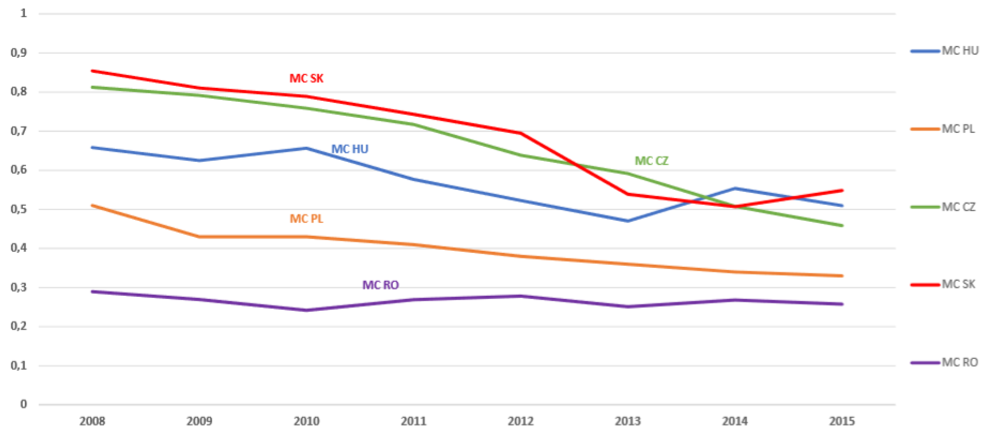
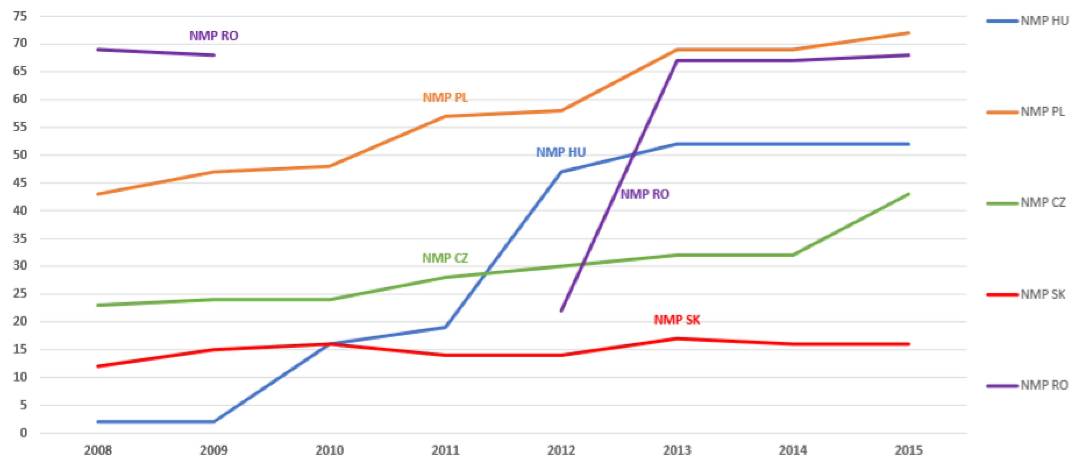
Since one of the main objectives of this paper is to analyze the correlation between market liberalization and competitiveness, we have selected factors that reflect the assumed higher intensity of competition. Market concentration is generally measured by the Herfindahl–Hirschman index (HHI) [23] and, for rail freight markets, applicable references exist, e.g., Crozet, 2016 [24]. Although in his paper, Crozet leaves the question open as to whether high market concentration in the rail freight industry should be regulated or whether this situation leads to high(er) competitiveness. He states that dominancy of one or some major operators might be abusing and thus likely decrease competitiveness. Based on this, we applied market concentration attributes such as calculated HHI, market share of the biggest player of the total freight volume, market share of the smallest market player and number of market players.

Determining connections between regulative actions and competitiveness was also among the objectives of our survey. There have been several notable attempts in the scientific literature concerning this issue including the case of the European railways [25,26]. In our study of East-Central European countries, we decided to apply a direct regulatory factor, namely, the annual number of railway-related legislative actions in these countries.

Considering the demand side, many authors (e.g., Jarzemskis and Jarzemskiene, 2017) stated [27] that higher competitiveness in rail markets does not necessarily originate from a higher intensity of competition in the market (in Lithuania there is only one rail freight operator so the market is monopolized and still has been proven to be more competitive internationally than Poland where the competition is higher) but from the existing demand of the destination sites. Thus, we selected factors such as import, export, and transit freight volumes, domestic freight volume and total rail volumes in million tons, all measured in national levels in the examined five ECE countries.

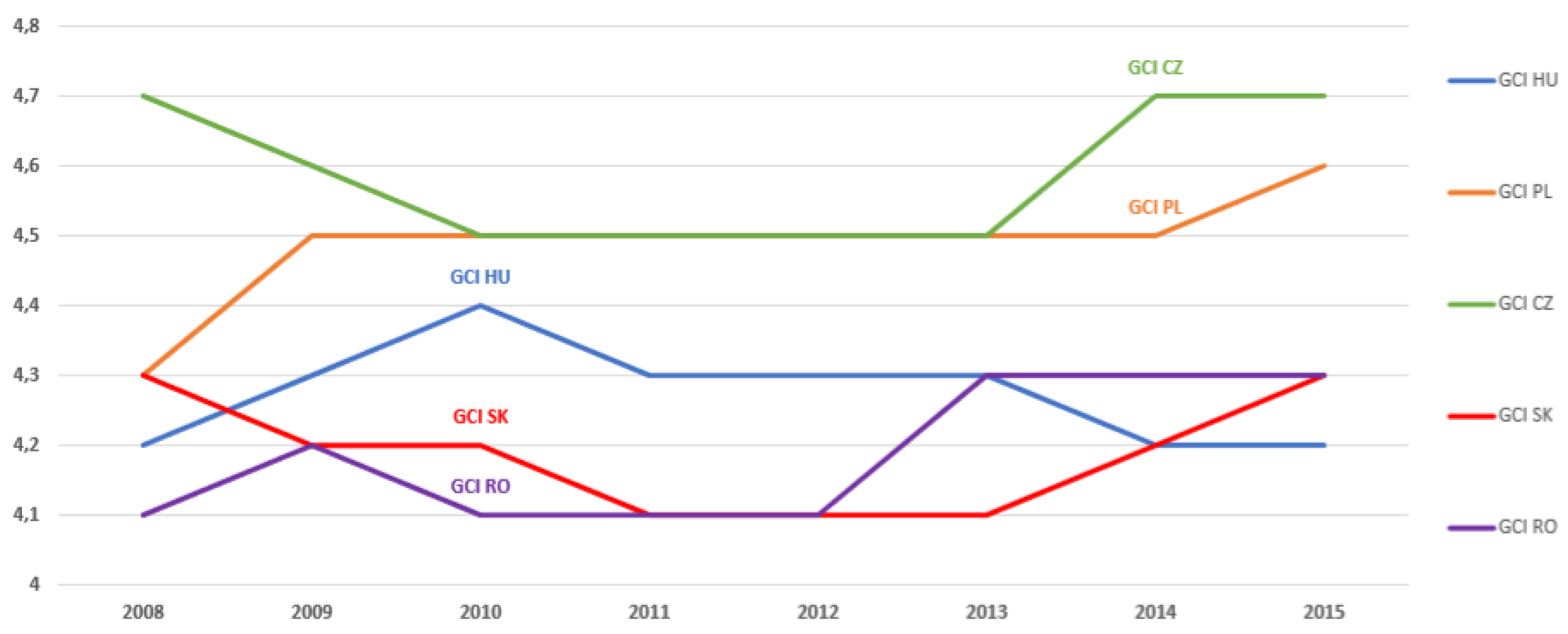
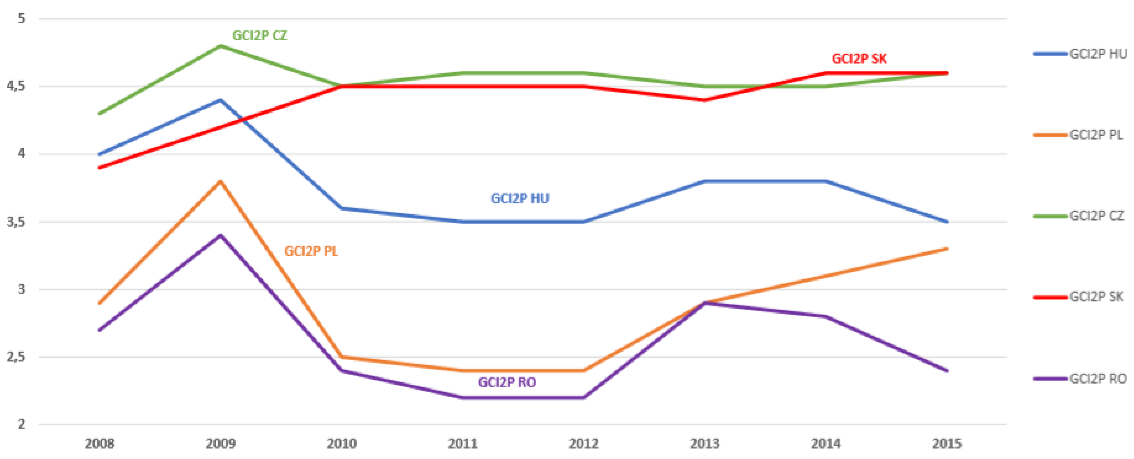
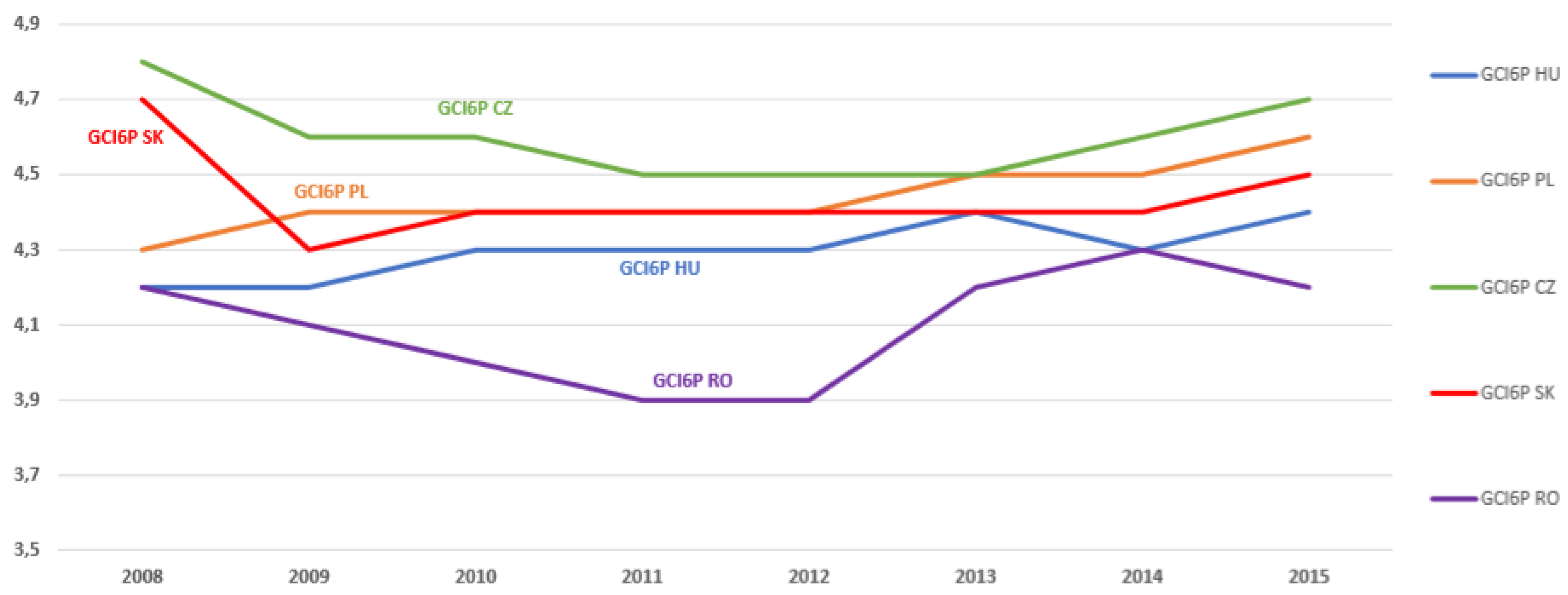
Finally, we selected a direct competitiveness index, GCI, which is also officially measured/calculated by European countries. GCI, constructed and applied by the World Economic Forum, is accepted worldwide for indicating market and country competitiveness, including several transport- and logistics-related composites [28]. In our study, we applied GCI as an all-encompassing attribute related to competitiveness of each examined country, the second pillar of GCI related to rail infrastructure quality specifically and the sixth pillar related to market efficiency (The Global Competitiveness report 2011–2012).

Based on the ones detailed in the literature review, concentrating merely on rail freight attributes, the following influencers were applied in the model (

Table 2. Influencing attributes applied to rail freight market competitiveness.

Attribute Number	Attribute Name	Contraction	[Unit]	Averages HU	Averages PL	Averages CZ	Averages SK	Averages RO
1	Biggest Market Player	BMP	percentage	77.0	50.0	80.0	80.0	47.0
2	Domestic Traffic	DT	mill. Tons	12,541	175,901	40,255	7398	46,207
3	Export	EX	mill. Tons	12,873	19,522	19,545	10,924	3207
4	GCI 6 Pillar (6) Goods Market Efficiency	GCI6P	no unit of measurement	4.3	4.3	4.6	4.5	4.1
5	GCI index	GCI	no unit of measurement	4.3	4.5	4.6	4.2	4.2
6	GCI 2. Pillar 2. 03 Quality Of Railway Infr.	GCI2P	no unit of measurement	3.8	2.9	4.5	4.3	2.7
7	Import	IM	mill. Tons	13,198	32,093	20,833	16,628	5874
8	International (Export + Import + Transit)	INT	mill. Tons	35,844	54,763	48,225	38,680	9521
9	Market Concentration	MC	percentage	0.6	0.4	0.7	0.7	0.3
10	Number Of Market Players	NMP	piece	24.0	55.0	27.0	18.0	22.0
11	Rail Share From The Total Vol.	RS	percentage	18.3	16.0	22.4	21.9	22.2
12	Smallest Market Player	SMP	percentage	0.0	1.3	0.5	0.0	0.0
13	Total Rail Traffic	TRT	mill. Tons	48,550	207,619	89,436	46,225	55,418
14	Track Access Fee	TAF	Euro	2.3	4.4	3.8	5.6	3.4
15	Transit Traffic	TT	mill. Tons	9772	3147	7846	11,127	439

). For better readability, we provide the 8-year average (2008–2015) values of each country for the 15 attributes, while the entire raw data table is presented in Appendix A of the paper.

3. Materials and Methods

In our research, countries are entities characterized by 15 attributes represented on different scales. The use of calculating the Euclidian distance between these entities in this high-dimensional space is non-applicable. Therefore, we have to use a method which reduces the number of dimensions of the space in a way that this reduction preserves as much information as possible.

Principal Component Analysis (PCA) is a statistical procedure that uses an orthogonal transformation to convert correlated variables into a set of linearly uncorrelated features which are called principal components [29].

The advantage of using PCA is twofold. On the one hand, a large attribute space can be compressed into a smaller space; on the other hand, it can be used in the visualization of the data with simple plots.

As for our case, in

Table 3. Correlation matrix (R) of the attributes.

	INT	EX	IM	DT	TT	MC	NMP	TRT	BMP	SMP	RS	TAF	GCI	GCI2P	GCI6P
INT	1	0.95	0.92	0.45	0.42	0.46	0.45	0.62	0.28	0.63	0.00	0.09	0.62	0.34	0.63
EX	-	1	0.84	0.47	0.29	0.42	0.49	0.63	0.23	0.61	0.01	−0.02	0.71	0.33	0.62
IM	-		1	0.74	0.08	0.18	0.63	0.85	−0.03	0.85	0.08	0.12	0.60	0.03	0.49
DT	-	-	-	1	−0.6	−0.43	0.80	0.98	−0.61	0.90	0.16	−0.06	0.36	−0.53	0.05
TT	-	-	-	-	1	0.76	−0.38	−0.40	0.81	−0.32	−0.19	0.13	0.02	0.75	0.40
MC	-	-	-	-	-	1	−0.44	−0.24	0.91	−0.27	0.26	0.49	0.20	0.71	0.48
NMP	-	-	-	-	-	-	1	0.81	−0.57	0.78	−0.14	−0.22	0.40	−0.33	0.24
TRT	-	-	-	-	-	-	-	1	−0.47	0.93	0.14	−0.03	0.45	−0.39	0.18
BMP	-	-	-	-	-	-	-	-	1	−0.5	0.15	0.31	0.06	0.76	0.35
SMP	-	-	-	-	-	-	-	-	-	1	0.01	−0.05	0.51	−0.26	0.21
RS	-	-	-	-	-	-	-	-	-	-	1	0.50	−0.07	−0.06	−0.02
TAF	-	-	-	-	-	-	-	-	-	-	-	1	−0.03	0.09	0.27
GCI	-	-	-	-	-	-	-	-	-	-	-	-	1	0.26	0.73
GCI2P	-	-	-	-	-	-	-	-	-	-	-	-	-	1	0.49
GCI6P	-	-	-	-	-	-	-	-	-	-	-	-	-	-	1

, it is clear that many of the attributes are highly correlated. This means that PCA can be used in order to reduce the dimensionality of the space that is the number of attributes. As a result, we will obtain a lower-dimension space defined by so-called PCA components, features or background variables.

The basic idea behind PCA is to compress the high-dimensional space into a lower-dimensional space such that it preserves as much variance as possible. After space compression into a convenient two-dimensional space, we can run a clustering algorithm in order to define clusters which group similar entities. This can help us analyze the connection between the different influencers (random variables) of rail freight market competitiveness and the entities. We expect that the representation in the two-dimensional space, defined by the obtained “background variables”, will help us better understand market competitiveness.

In the following, we will present the main steps of the method, and we relate the steps to our practical problem.

Let us suppose we have n entities in an ${ℝ}^p$ space. Each entity is characterized by p variables ($X_1,\dots ,X_p)$. Based on this, an X matrix of nxp dimensions can be constructed in which $x_{ij}$ numbers denote the value of the j-th variable in the i-th entity, the rows correspond to entities, and the columns correspond to variables.

The application of PCA has two main points of interest. The first one is related to the case of the entities when we use the rows of the X matrix. The second one is related to the case of the variables (attributes) in which we deal with the columns of the X matrix.

The fact that the variables are measured on different scales poses a regular problem. To overcome this drawback, we standardize the values as follows. We calculate the arithmetic means and standard deviations of each variable then the standardized values are computed by Formula 1.

$$z_{ij}=\frac{x_{ij}-{\overline{x}}_j}{s_j}$$

(1)

where $\overline{x_j}$stands for the mean value and $s_j$ for the variance of variable j.

Note that the final objective of PCA is substituting $X_1,\dots ,X_p$ by the principal components $C_1,\dots ,C_p$ and then reducing the p dimension by selecting the principal components with the highest explanation powers (of variance) and omitting the rest.

It is easy to see that the new variables $Z_j$ associated with the columns will have 0 mean and all the standard deviations equal to 1.

3.1. Phase 1. PCA Applied to the Entities

Two entities are similar when they are close to each other in the p-dimension space.

In this subsection, we want to find the lower dimension space, where the entities (points associated with the row vectors of X) are projected in the space defined by the principal components such that as much variation as possible is preserved. First, we define the first axis for which the sum of squares of projections is maximal. We denote this by u1, then it can be proved that the two-dimensional plane with this property is determined by u1 and u2 which is orthogonal to u1. The projection of the entities in the plane are called scores. If two scores are close, then the entities have similar properties.

Now we consider the projections of each entity i to the component k. We denote this by $F_{ik}$. The vector with coordinates $F_{ik}, i=1,\dots n$ is denoted by ${\mathit{F}}_{.\mathit{k}}, k=1,\dots p.$ We obtain, for each component, an n dimensional vector since we projected n points.

3.2. Phase 1. Variables Represented in the Space Defined by the Principal Components

In this subsection, we express the correlation between $\mathit{x}{.}_{.\mathit{k}}, k=1,\dots p$, which are the column vectors of the X matrix corresponding to the variables (attributes) and ${\mathit{F}}_{.\mathit{k}},k=1,\dots ,p$. If we project only into the two-dimensional space defined by the two principal components, then we calculate the correlations between $\mathit{x}{.}_{.\mathit{k}}, k=1,\dots p$ and ${\mathit{F}}_{\mathbf{.1}}$, respectively $\mathit{x}{.}_{.\mathit{k}}, k=1,\dots p$ and ${\mathit{F}}_{\mathbf{.2}}$, In this way, variable $\mathit{x}{.}_{.\mathit{k}}$ has the coordinates $r\left({\mathit{F}}_{\mathbf{.1}},\mathit{x}{.}_{.\mathit{k}}\right)$ respectively $r\left({\mathit{F}}_{\mathbf{.2}},\mathit{x}{.}_{.\mathit{k}}\right)$. This means that the variables are projected inside a circle with a unit radius of 1 known as the correlation circle.

Since one of the main objectives of PCA is to determine which variables are correlated to each other, we need the correlations matrix between the variables. The covariance of the standardized j-th variable and the standardized l-th variable is:

$$s_{ij}=\frac{1}{n}{{\displaystyle \sum }}_{i=1}^n{z}_{ij}{z}_{il}j, l=1,\dots p$$

(2)

The strength of the linear relation between two variables (attributes) of a particular phenomenon is expressed by the correlation coefficient:

$$r_{jl}=\frac{s_{jl}}{s_j{s}_l}$$

(3)

where 0 ≤ │r_jl│ ≤ 1.

The closer the absolute value of r_jl lies to the unit, the stronger the linear relationship between the two variables is. This is the basis behind formulating the model through linear functions. From a geometrical point of view, the correlation between the centered variables represents the cosine of the angle ${\theta }_{kl}$between the vectors associated with the two variables.

$$cos \left({\theta }_{kl}\right)=r\left(x_l,x_k\right)$$

(4)

The problem is that these variables are in a high-dimensional space. So, it is impossible to interpret the angles and therefore the closeness between the variables. The idea is to project these variables onto a two-dimensional space. Based on their projection and with the help of the angles we obtain between the projections, we can obtain information on which of the variables are “close” to each other.

We emphasize here that only those variables which have an associated vector width and length close to 1 are deemed well represented. If not, then those variables are not well represented and the angles which appear are not meaningful. We used this in our data analysis.

The low-dimensional space can also be created in a way that it retains as much variance as possible.

Let us consider the correlation matrix:

$$R=\left(\begin{array}{cccccc}1& r_{12}& \dots & r_{1l}& \dots & r_{1p}\\ r_{21}& 1& \dots & r_{2l}& \dots & r_{2p}\\ ⋮& ⋮& & ⋮& & ⋮\\ r_{j1}& r_{j2}& \dots & r_{jl}^{}& \dots & r_{jp}\\ ⋮& ⋮& & ⋮& \dots & ⋮\\ r_{p1}& r_{p2}& \dots & r_{pj}& \dots & 1\end{array}\right)$$

(5)

Accordingly, the correlation matrix and for Formulas (2) and (3) the correlation matrix can also be written as follows:

$$R=\frac{1}{n}{Z}^{T}Z$$

(6)

The R matrix for the standardized variables will be used to determine the principal components.

3.3. Phase 2. Determination of the Principal Components

The idea is to find the component v1 such that

$$v_1=argma{x}_v{\displaystyle \sum }_{k=1}^{p}r{\left(v,z_k\right)}^2$$

(7)

And then find the direction $v_2$ orthogonal to it and so on. These directions are orthogonal to each other and have the property of maximizing the variance of the projections.

The principal components can be found by singular value decomposition or by diagonalizing the correlation matrix to extract the eigenvectors and the eigenvalues. We denote by ${\mathit{u}}_s$ the eigenvectors corresponding to the eigenvalues ${\lambda }_S$. Let us note that ${\lambda }_S$ represents the variance of the entities projected to the ${\mathit{u}}_s$ component. The eigenvalues will appear in decreasing order.

3.4. Phase 2. The Representation of the Entities and Variables

The representation of the entities with respect to the attributes are expressed by the scores with respect to the loadings in the following two formulae:

$$F_{is}=\frac{1}{{\lambda }_s}{{\displaystyle \sum }}_{k=1}^p{z}_{ik}{G}_{ks},\mathrm{coordinate}\mathrm{s}\mathrm{for}\mathrm{entity}i$$

(8)

$$G_{ks}=\frac{1}{{\lambda }_s}{{\displaystyle \sum }}_{k=1}^p{z}_{ik}{F}_{is} \mathrm{coordinate}s\mathrm{of}\mathrm{the}\mathrm{variable}k$$

(9)

These formulae imply the very important conclusion that entities are on the same side as their corresponding variables with high values.

Some important concluding assertions:

• The entities which have close projections have similar attributes, the entities which are far from each other are different in their subsets of attributes.
• Attributes (variables) that are close to each other correlate in a similar way with the principal components, i.e., their angle with the principal components is similar (see Figure 1).
• The attributes are projected in the subspace of the two principal components such that their length is maximum 1. Variables that have lengths close to 1 are well represented and can be interpreted in this subspace (Figure 1).
• The entities that are on the same side as each other have corresponding variables with high values. If the entities are in the opposite direction to each other, then they have small values for these variables.

Based on these assertions, we can analyze our rail freight-related dataset and formulate some findings.

4. Results

Following the general procedure of the PCA, first, the standardized raw data matrix must be constructed. In our case, the 15 influencing factors, as Table 2 demonstrates, are the variables. So, the value of p is 15. The entities are the countries, whose freight market data we gathered from 2008 to 2015 (we were able to obtain a reliable complete dataset only for this period to include all countries for all 16 factors). So, the number of entities is five times eight (the number of years). Thus n = 40 in our model. All five countries had liberalized their rail freight market by the initial date of the examined period.

Afterwards, we constructed the R correlation matrix of the 15 variables, presented in Table 3. Elements under the main diagonal represent the density plots of the pair of random variables. Elements on the diagonal represent the histograms of the univariate variables.

For the scope of this study, the elements above the main diagonal are the most essential; they are the pairwise correlations of the variables.

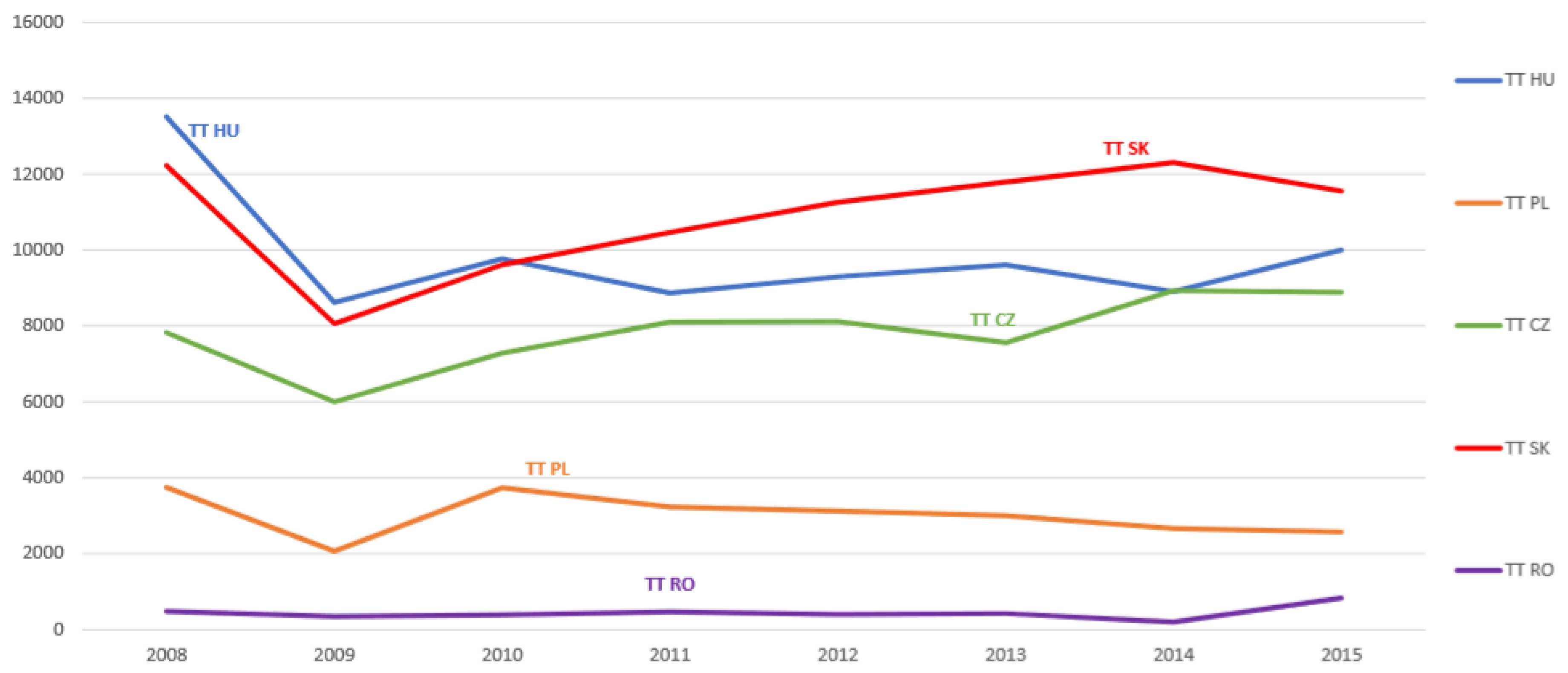
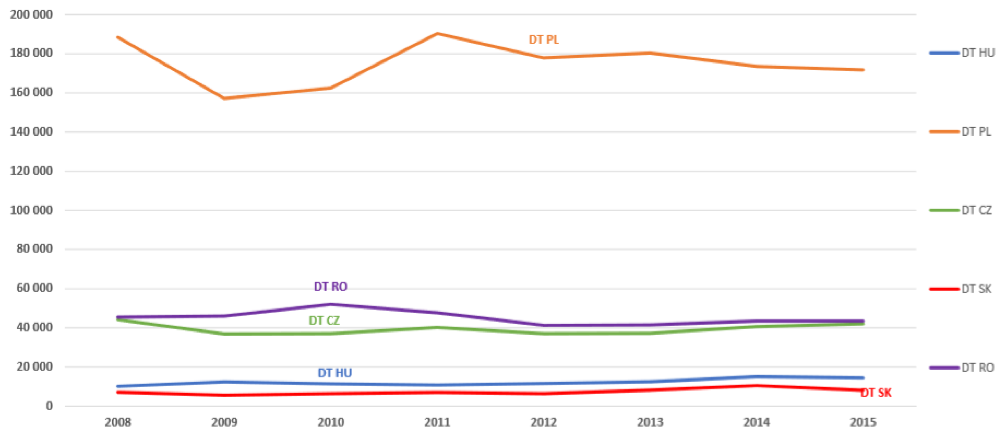
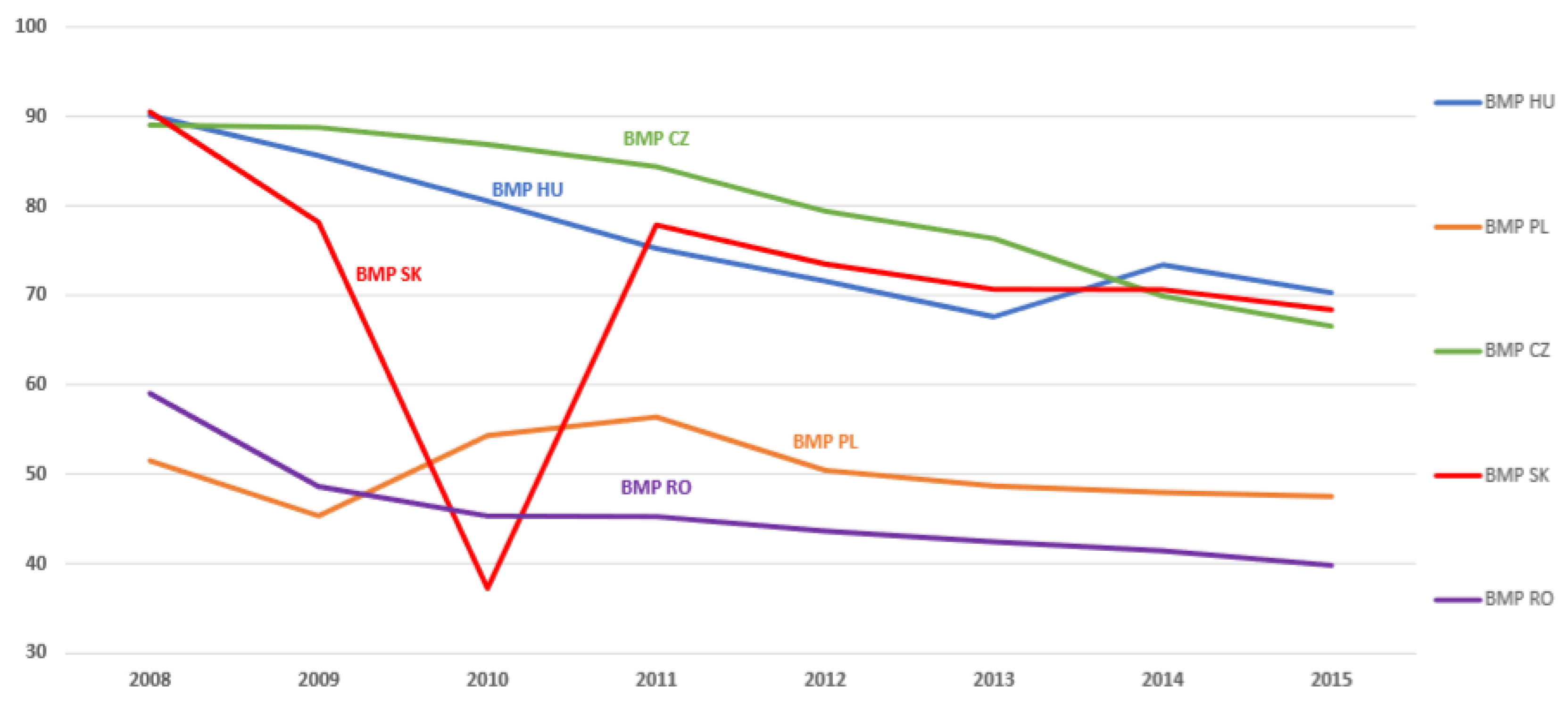
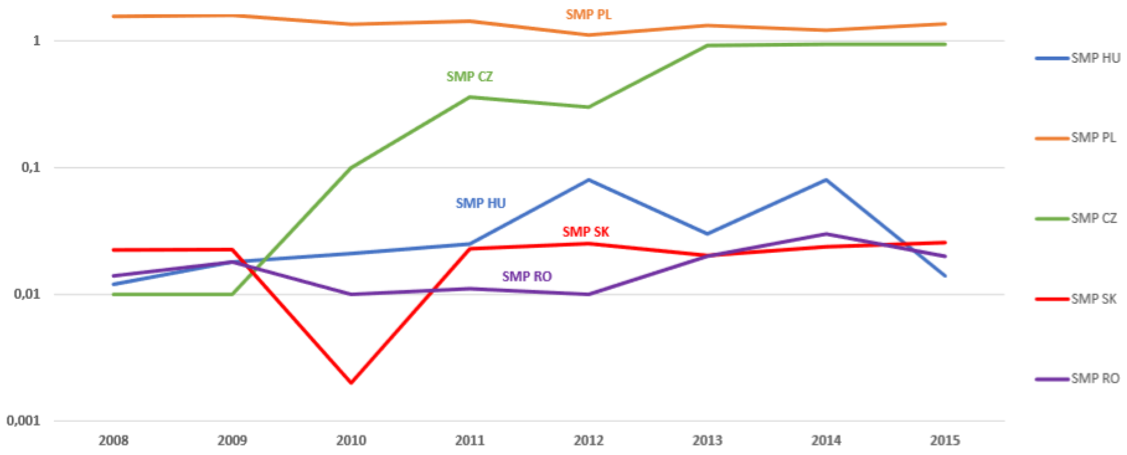
Table 3 justifies the selection of PCA, since it demonstrates not only the high degree of correlation of the analyzed attributes, but also the complexity of these interrelations. This complexity can be interpreted more appropriately by the reduction in dimensions applying PCA. The data represented in this table are official data of the five Central-European countries through eight years. Strong correlation (over 0.8) could be detected—except for the rather trivial ones—between some pairs of attributes. Interestingly, the percentage share of the smallest market player out of the total rail freight volume of the country (SMP) is in strong correlation with domestic traffic (DT, intensity: 0.9); import (IM, intensity: 0.85) and total rail traffic (TRT, intensity: 0.93). Moreover, the number of market players (NMP) is strongly correlated with domestic traffic (DT, intensity: 0.8) and total rail traffic (TRT, intensity: 0.8). Furthermore, between the percentage of the biggest market player (BMP) and transit traffic (TT, intensity: 0.81), a strong correlation could also be detected. This could suggest that the composition of the rail freight market in terms of the size of its competitors has an impact (or at least interrelation since we do not know the direction of the effect) on domestic, import and transit traffic (Figure 2). It is also exhibited in Table 3, that the directly measured market efficiency (by GCI 6th pillar, GCI6P) is correlated with international and export freights (which was quite expectable), but also interrelated with market concentration (MC) with the third strongest intensity, 0.48. The direct measure of rail infrastructure quality (GCI 2nd pillar, GCI2P) is bounded to total traffic, which is quite obvious. However, there is also significant correlation between GCI2P and market concentration (0.7) and the biggest market player (0.76). Based on the above, PCA is worth performing in order to reveal more complex interrelations of the variables and their connections to the entities.

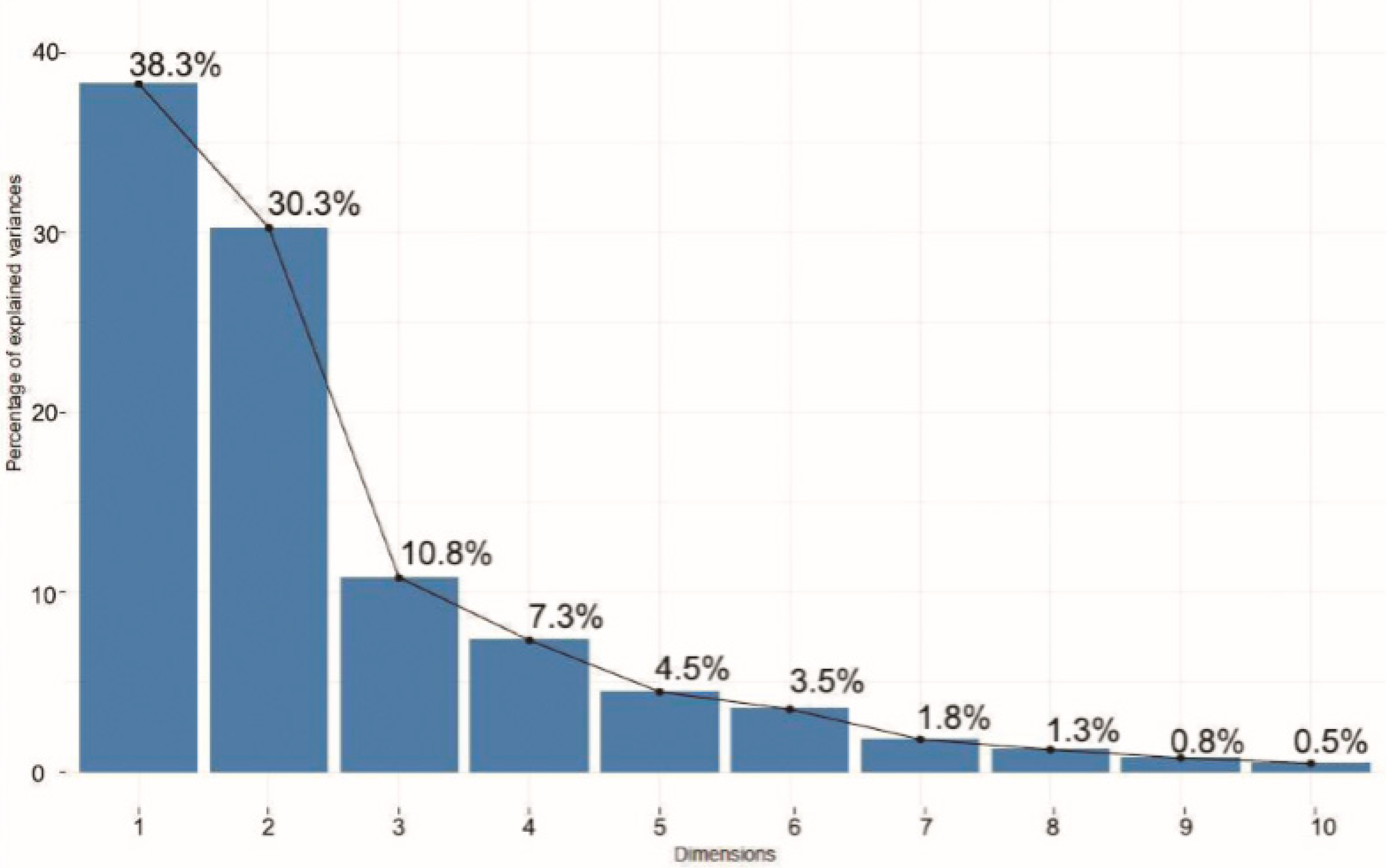
Applying Formulas (4) and (5) described in the Methodology section, the steps of principal components determination can be conducted. In our case, the 16 influencers are substituted by 16 principal components. After reducing the dimensions, only those principal components remain in the model, which explains the dominance of the total variance (this could be reached by determining the eigenvalues because it can be proven that the standard deviation of the principal components equals the square root of the eigenvalues). Having calculated the unstandardized first and then the standardized principal components, the following was deduced.

Figure 3 shows that the first two principal components explain 67% of the total variance. Thus, selecting these two can be sufficient for the analysis. Therefore, the space generated by PC1 and PC2 (which is a rotated and projected space now compared to the original 15-dimensional space of the raw variables) is applied to describe the interrelations of the variables and entities. The first three principal components would have explained 79.5% of the total variance but the contribution of the third one would only have been 10.8% and the interpretation of the results would have been much more difficult in a three-dimensional space so we decided to consider the first two principal components. 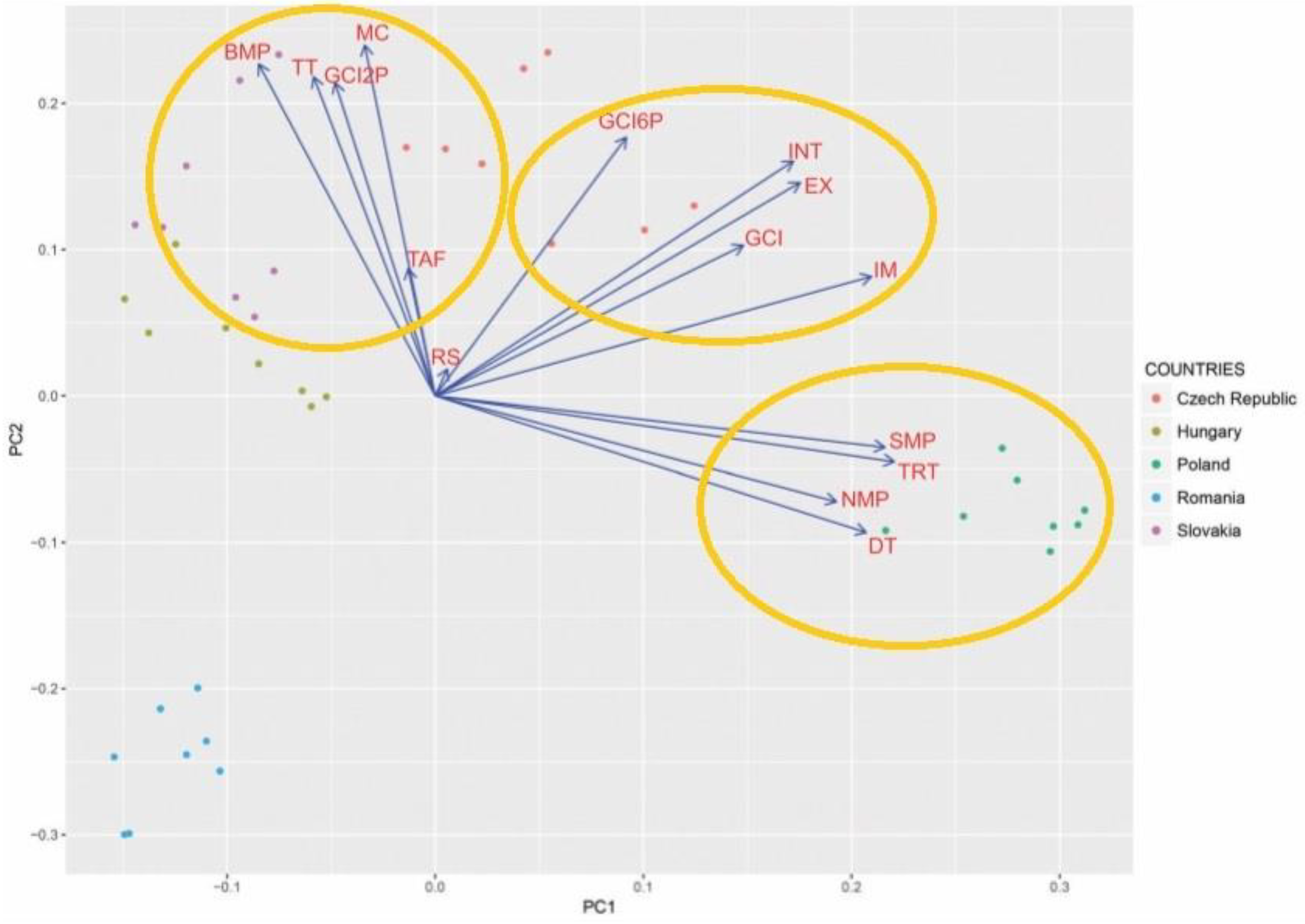Figure 1 exhibits the situation of the 15 attributes in this two-dimensional space.

The PCA technique constructed two axes, PC1 and PC2, and the proximity of the attributes demonstrates the weight of each variable in the linear combination for the construction of PC1 and PC2. Consequently, in the case of PC2, the attributes ‘Biggest market player’ and ‘Market concentration’ play the most significant roles (these have the highest PC2 coordinates). Based on this, the “shadow attribute” is most likely the degree of liberalization (not legislative but the real situation). For PC1, the most significant attributes are ‘Total rail traffic’, ‘Smallest market player’, ‘Import’ and ‘Domestic traffic’. Evidently, PC1 “shadow attribute” is the quantity of rail transport, measured in tons. It is interesting that the ‘Smallest market player’ has significant weight in constructing the PC1 axis.

We note that some conclusions can be drawn by the directions of the vectors in this space. Opposite direction means negative correlation of an attribute on another or between an attribute and an axis. Also, the position of the entity points means positive or negative correlation with the others in the constructed PCA space. In our case, the Romanian points (marked with light blue color) are remote from the other ones in the negative area of the coordinate space, which means that their data correlate negatively with the other countries’ data.

Another remarkable issue in PCA is that in the created space, the position of the attributes shows the degree of their correlation. If two variables are close to each other, that means they are strongly interrelated. Based on this, the strong interrelation of transit traffic and the quality of railway infrastructure is visible and also the connection between the smallest market player and the total rail traffic. The proximity of ‘International traffic’ and ‘Export’ indicates that the majority of railway transport in Eastern-Central European countries is motivated by export transportation.

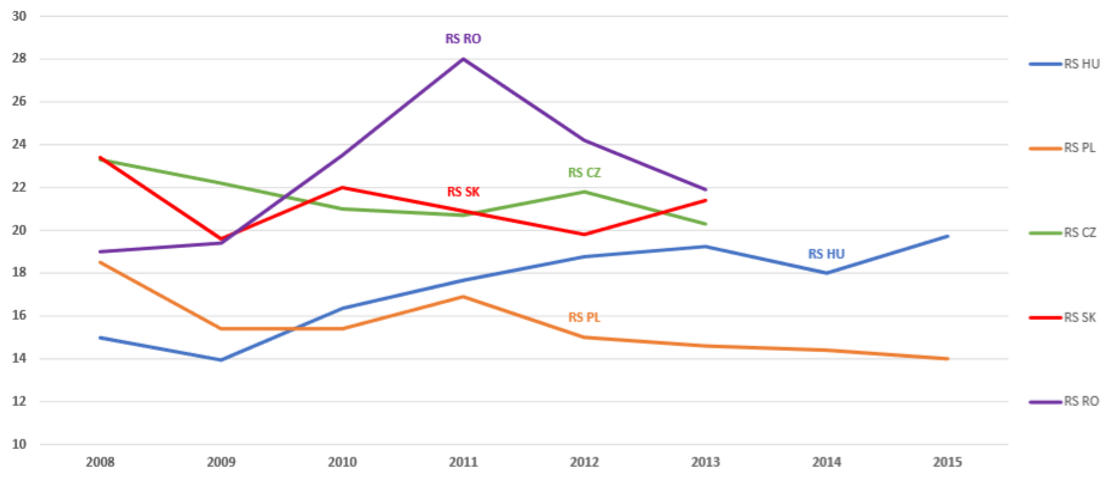
In Figure 1, we consider only the variables for which the associated vectors have lengths close to one (in the current scaling, 0.1). Only those vectors are well represented, so ‘Rail share’ and ‘Track access fee’ can be omitted from the PCA analysis, their projection is not significant in the constructed vector space of PC1 and PC2 axis. One can observe that in Figure 3, three main attribute groups can be determined.

The first consists of biggest market player (BMP), transit traffic (TT), quality index of infrastructure (GCI2P), market concentration (MC) and track access fee (TAF) can be also connected here. This group demonstrates best the intensity of freight competition. If the market is very concentrated and the biggest company is very dominating in the C-E region, then high infrastructure quality and low fees could be expected with big volumes of transit traffic.

Market efficiency (GCI6P), international traffic (INT), export (EX), import (IM), rail share (RS) and the global competitiveness index (GCI) constitute the second group of variables. This group can be called international competitiveness indicators, since GCI is a direct measure of it and the others all reflect the global capability of the national rail system. Based on the conducted PCA, however, market liberalization and thus market concentration have no serious impact on the international competitiveness, because there is no significant correlation between this second group and the ‘Market Concentration’ and ‘Number of Market players’ attributes. However, increasing market efficiency instead of further liberalization might have a positive impact on the international competitiveness of the countries, which supports the findings of Bougna and Crozet (2016) cited in the Introduction. The third group consists of domestic traffic (DT), smallest market player (SMP), number of market players (NMP) and total rail traffic (TRT). Hence, we can conclude that for national rail freight, the existence of small freight forwarders is essential and has a positive impact on the total rail freight performance. In conclusion, market liberalization implementation should concentrate on motivating the small forwarders in order to increase domestic traffic, but it does not contribute to international competitiveness.

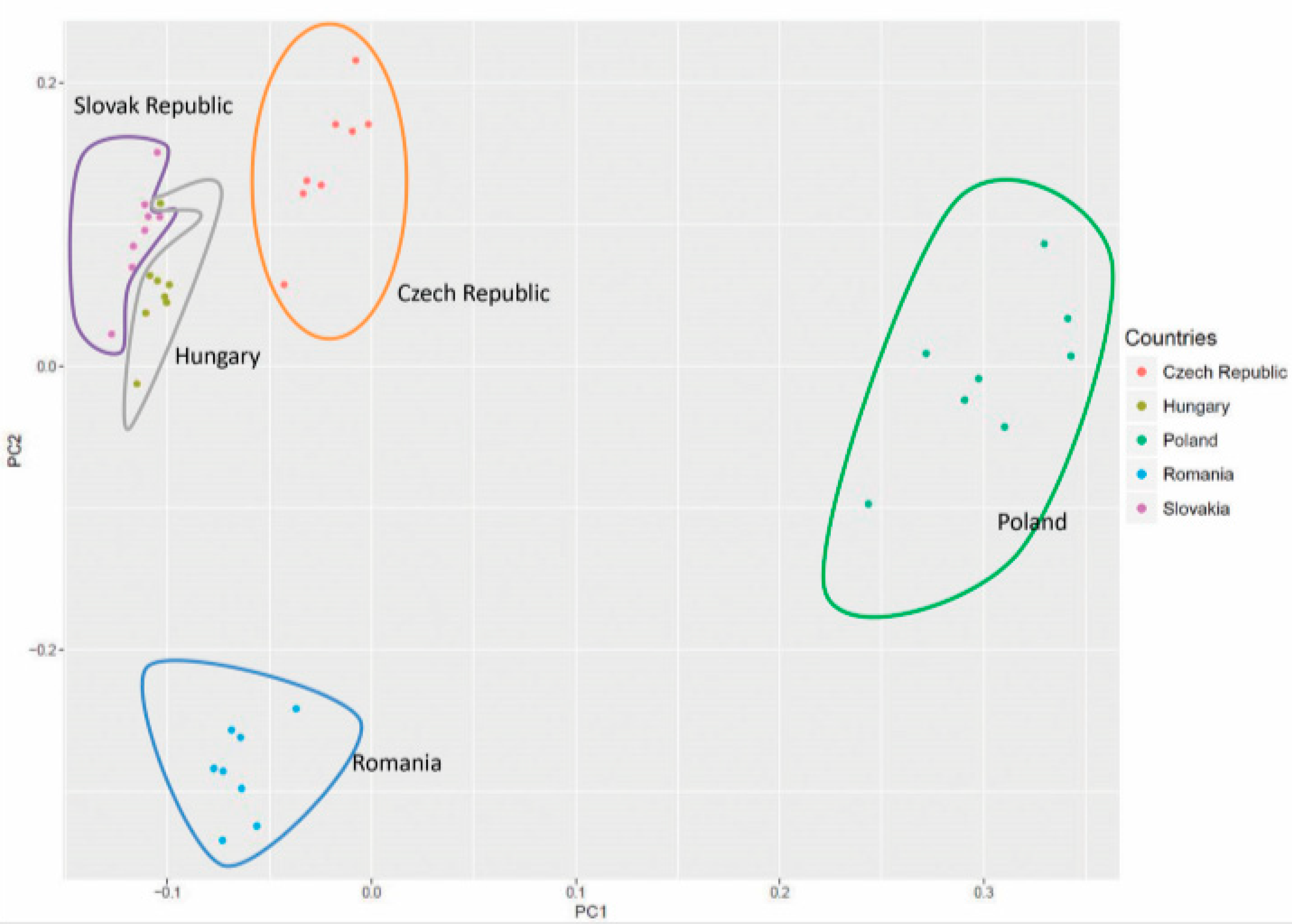
Figure 1 also includes the positions of the examined five Eastern-Central European countries in the two-dimensional principal component space. The results strengthen the findings of Feuerstein et al. [14], who stated that different competitiveness influencers have different impact and importance in EU countries. Based on the attribute effects, the clusterization of the examined national rail freight markets can be completed—for better visualization, we constructed Figure 2.

National characteristics can be easily detected in this figure. Since the rail freight market of Poland is very much related to the other examined countries, in their case domestic factors are dominant. For Slovakia and Hungary, transit traffic is very important. So, their position is situated near the transit factors. The Czech Republic is also situated next to transit-like factors but also close to international competitiveness variables. Romania seems to be in the opposite direction to the variables, meaning that it is characterized by low values for these variables, which can be explained by the relative closeness of its rail freight market (lower proportion of international freight volumes) and different features compared to the other Eastern-Central European countries.

Regarding the recommended national transport policy implications, Figure 1 is also rather telling. For Slovakia and Hungary, measures related to infrastructure developments and market concentration (focusing on the biggest participants of the competition) can be the most effective in terms of raising competitiveness. As for the Czech Republic, market efficiency issues have to be prioritized. In Poland, the situation of small freight forwarders is the most crucial issue and many more small rail freight companies would be necessary. For Romania, further expansion of the railway to international traffic can be recommended.

The analysis revealed the interrelation of market liberalization and international competitiveness in a way that the roles of cause and effect are not trivial. Based on the results of the correlations of influencers and positions of countries, we can state that market liberalization issues do not necessarily cause increased international competitiveness in the rail market. Merely opening the market and motivating new players to enter in the market does not automatically cause higher competitiveness; see the different/opposite cases of Poland and Hungary. Because of the complex relations between railway attributes and the relative remote positions of liberalization and competitiveness influencers demonstrated by PCA, and also considering the significant distance between the examined countries, we emphasize the need for country-specific analyses before taking market liberalization measures.

5. Conclusions

Improving railway markets is essential both from economic and sustainability perspectives, which have been recognized by many states all over the world. However, the best ways of raising rail competitiveness are not trivial and need thorough analysis because a general solution may not exist for the different cases of national markets.

This paper aimed to contribute to the ongoing debate about the relation of rail freight market liberalization and competitiveness by applying the complex multivariate method of PCA. The contradiction between the high expectations of railway market liberalization and the stagnation of the Central-Eastern European rail freight sector has been palpable in recent years. The findings of our analysis can partly explain this discrepancy.

Our results support the findings of Bougna and Crozet in terms of international competitiveness; dealing with market efficiency questions appears to be more important than the drive for liberalization. However, for domestic rail freight markets—especially in countries with big volumes of rail freight and a large national market—focusing on small forwarder companies can be even more advisable.

Rail infrastructure developments contribute most directly to transit traffic and, in these cases, the biggest rail forwarders play the most significant role.

National characteristics of railway markets could be also detected, which supports the robustness of our study results.

Furthermore, the statements of Zunder et al. (2013) [30], that liberalization alone cannot explain the different rail freight performance of the countries in the EU, have also been verified. They found that organizational and managerial bottlenecks strongly determine this performance and, thus, market competitiveness. Our results support this idea as market concentration and market efficiency issues have not been positioned closely in our PCA vector space. Thus, liberalization measures cannot be the only means to improve rail freight performance.

Involving more data from databases of other countries (from other regions beyond the territory of the European Union or analyzing the data of old EU members but regarding a different period due to their earlier liberalization) might be a promising subject of further research and also selecting and integrating other attributes might improve on our findings in the future.