Research in Meteorological Modeling Oriented Comprehensive Surface Complexity (CSC)

Abstract

Ground surface characteristics (i.e., topography and landscape patterns) are important factors in geographic dynamics. Thus, the complexity of ground surface is a valuable indicator for designing multiscale modeling concerning the balance between computational costs and the accuracy of simulations regarding the resolution of modeling. This study proposes the concept of comprehensive surface complexity (CSC) to quantity the degree of complexity of ground by integrating the topographic complexity indices and landscape indices representing the land use and land cover (LULC) complexity. Focusing on the meteorological process modeling, this paper computes the CSC by constructing a multiple regression model between the accuracy of meteorological simulation and the surface complexity of topography and LULC. Regarding the five widely studied areas of China, this paper shows the distribution of CSC and analyzes the window size effect. The comparison among the study areas shows that the CSC is highest for the Chuanyu region and lowest for the Wuhan region. To investigate the application of CSC in meteorological modeling, taking the Jingjinji region for instance, we conducted Weather Research and Forecasting Model (WRF) modeling and analyzed the relationship between CSC and the mean absolute error (MAE) of the temperature at 2 meters. The results showed that the MAE is higher over the northern and southern areas and lower over the central part of the study area, which is generally positively related to the value of CSC. Thus, it is feasible to conclude that CSC is helpful to indicate meteorological modeling capacity and identify those areas where finer scale modeling is preferable.

1. Introduction

Characterization of surface complexity is essential throughout the earth sciences, since each geographic process operating at the ground surface encounters and affects the ground surfaces (i.e., topography, land use and land cover, soil) [1]. Given this significance of the ground surface, the complexity is widely applied in many different scenarios, such as identification of active landslides based on topographic complexity [2], design of multiresolution approach to estimate snow water equivalent [3], and so on. Similar to these study, this paper analyzes the surface complexity to describe the spatial heterogeneity of ground surface in a specific area. To quantify the surface complexity, a number of different techniques have emerged over the years, although they usually focus on one of the variables, including topography, land use and land cover [4,5], and so on.

From the perspective of topography, usually topographic complexity (TC) is considered to be the same as surface roughness, representing the degree of the difference in elevation among the adjacent cells of a digital elevation model (DEM). The topographic complexity index (TCI) is derived to reflect the average elevation change between any point on a grid and its surrounding areas [6]. This TCI is widely applied in geographic research. For instance, Li et al. [7] argued that the uncertainties in volume calculations based on a DEM are primarily related to the discrete error, which is usually caused by DEM resolution and the TCI. In the dynamic process simulation, the TCI is also considered to achieve better simulation performance. In meteorological simulation, the modeling accuracy is related to the TCI of the study area, since the presence of complex terrain causes spatial (in both horizontal and vertical directions) and temporal variations in air flow and turbulence, which strongly influence the meteorological conditions [8].

Concerning land use and land cover (LULC), the structural complexity of LULC is essential for the analysis of the patterns in structural elements and processes that occur [9]. On the one hand, it is highly relevant to the accuracy of data collection. When LULC information is obtained using satellite images and the proposed spectral-temporal-spatial classification method is applied, the results are of highest to lowest classification accuracy with different land cover complexity, including South Dakota, Illinois, and Texas [10]. On the other hand, research utilizing LULC data is also affected by the LULC complexity [11]. Studies of ecosystem service (ES) maps indicate that the utility of coarse LULC data for ES mapping is limited to relatively homogeneous landscapes and that reliance on finer resolution LULC data may alter the estimated ES values [12]. Thus, a set of (landscape) indices was developed to quantify the LULC complexity. For instance, Miller and Brewer [13] applied hydrologically relevant landscape metrics to represent the diversity of LULC to refine flood estimation in urbanized catchments.

Along with the extensive research into dynamic geographic processes [14,15], increasing number of geographers realize that ground surface characteristics (i.e., topography, landscape patterns, vegetation, and soil) may imperatively affect the modeling of meteorological processes, hydrological processes, and so on. Since most processes represented in dynamic models are nonlinear, a change in spatial resolution of model can introduce bias in the simulated variables [16]. On the one hand, fine resolution simulations can provide fine-scale process representation but can be costly to apply over large domains. On the other hand, coarser spatial resolutions are more computationally inexpensive but at the expense of fine-scale model accuracy. In this context, surface complexity is proposed to facilitate multiresolution modeling, with finer resolution modeling covering the area with more complex surface complexity [17]. However, to our knowledge, such surface complexity for meteorological process modeling has never been done, although it is well known that meteorological modeling is highly affected by the surface condition, including topography and LULC [18,19].

The objective of this paper is therefore to propose a simple index—comprehensive surface complexity (CSC)—to coherently quantify the heterogeneity of topography and LULC for meteorological modeling and to compute and compare the complexity for different study regions in China. The remainder of the paper is organized as follows. Section 2 provides a brief introduction of the study area and the data used to express the topography and LULC. Based on topographic index and landscape index, Section 3 presents the quantification method of CSC, the CSC metrics for the study areas, and thoroughly analyzes the scale effect from moving window size. Section 4 presents one application of CSC indicating the meteorological modeling performance. The article finishes with a discussion and summary.

2. Study Area and Data

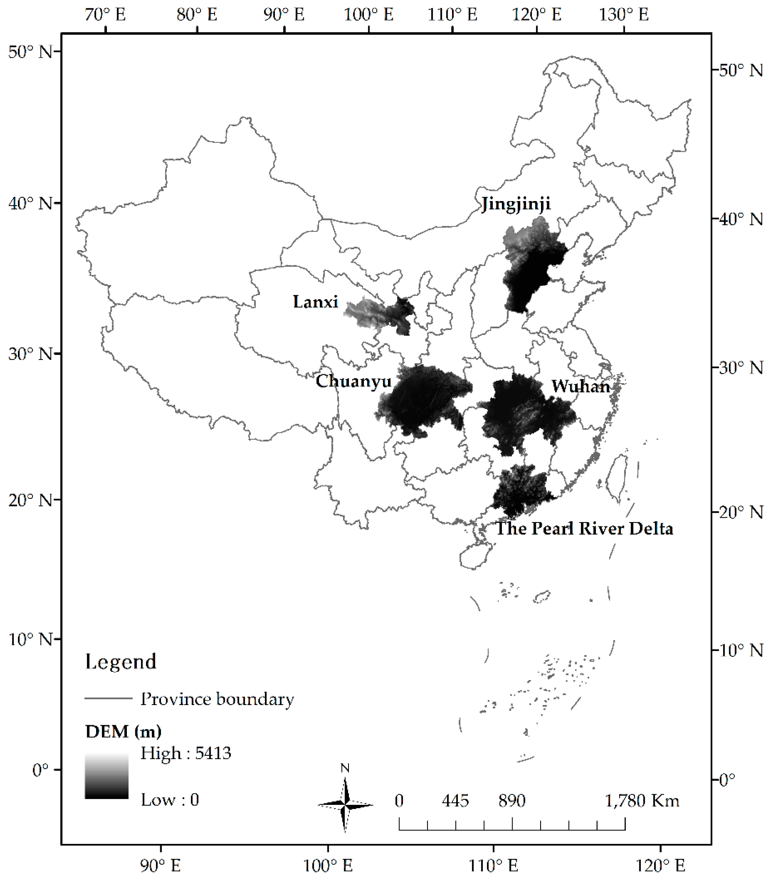
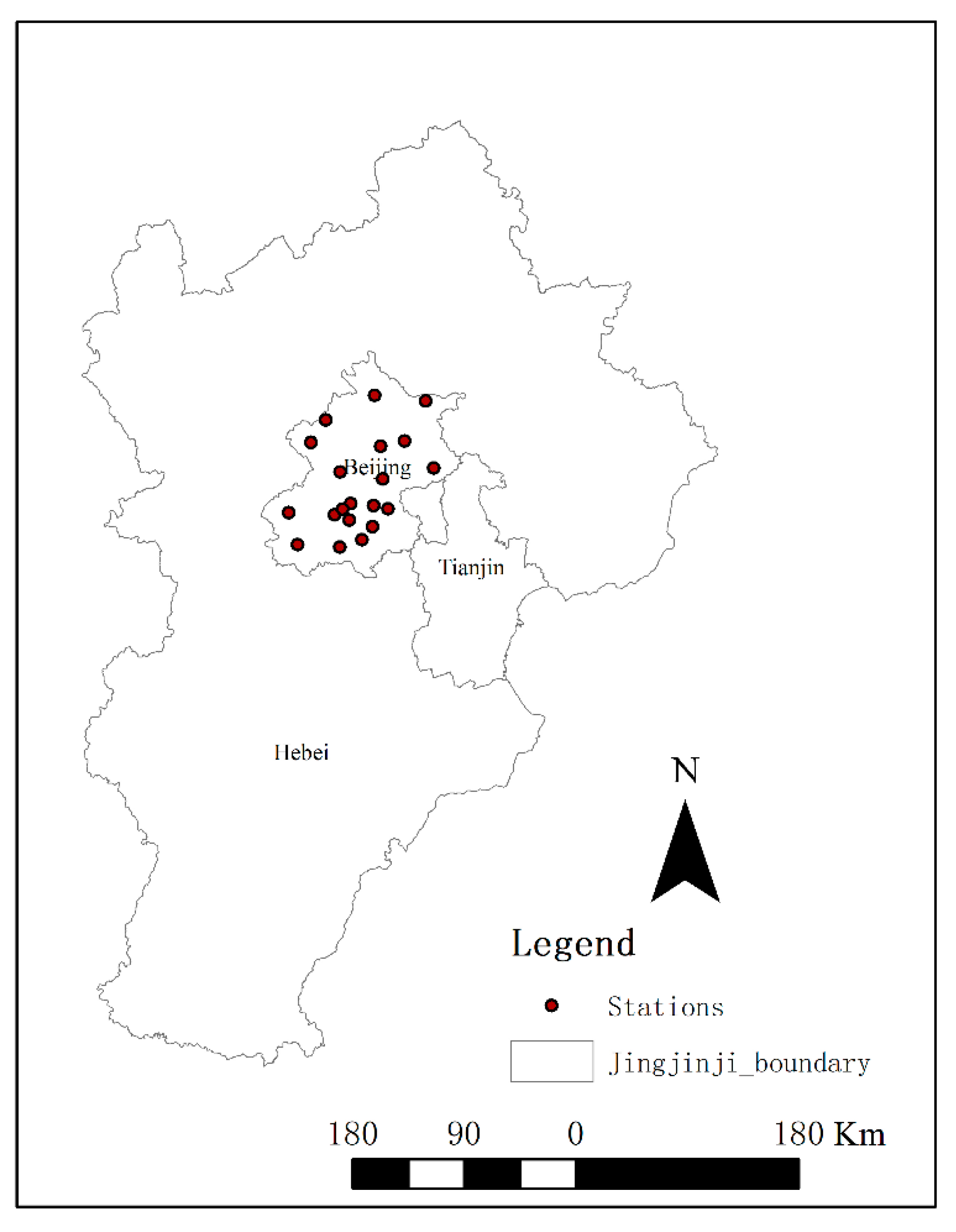
2.1. Study Area

This study focuses on five urban agglomerations of China (Figure 1): Beijing-Tianjin-Hebei urban agglomeration, Lanzhou—Xining-Yinchuan city area, Triangle of Central China, Chengdu-Chongqing City Group, and the Pearl River Delta. To make the areas readable, this paper marks the regions as Jingjinji, Lanxi, Wuhan, Chuanyu, and the PRD, respectively, instead of using acronyms. These urban agglomerations are of high population, accounting for nearly one-third (27%, in 2014) of the total population of China. Because of the intense impacts induced by human activities, the environment and ecosystem here are vulnerable [20] and meteorological modeling is widely studied. The study area has diverse climate conditions, including temperate monsoon, semi-humid/semi-arid continental monsoon, subtropical monsoon climate, and so on. Concerning such high populations, fragile environments, and various types of climate, this area deserves our attention to quantify the ground surface characteristics to provide information for geographic process modeling.

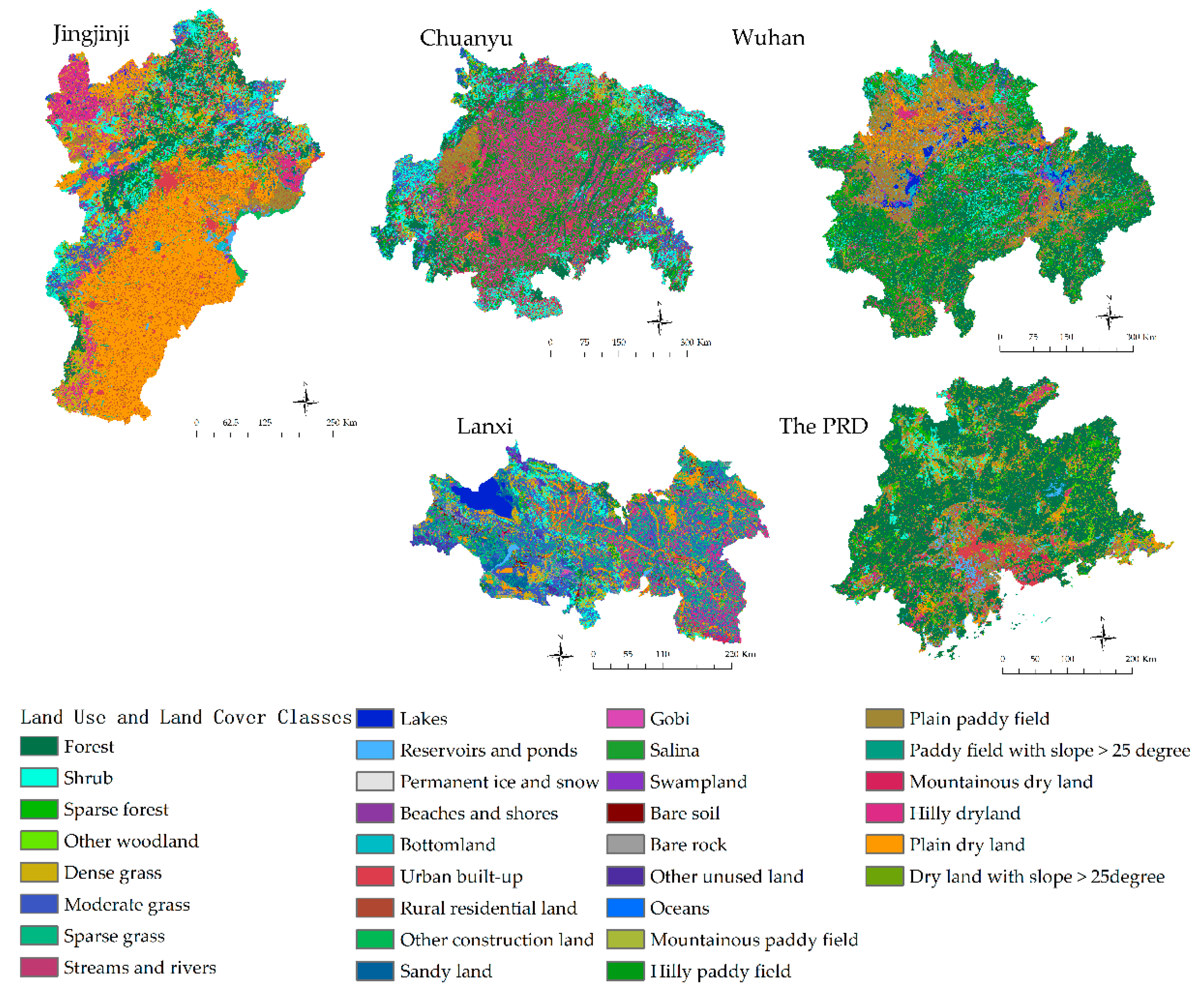
2.2. Topographic and LULC Data

The initial DEM data were derived from the Shuttle Radar Topography Mission (SRTM) data with a horizontal grid spacing of 90 m [21] (Figure 1). The DEM data were then aggregated to 1 × 1 km resolution using simple averaging aggregation in ArcGIS version 10.0, so that it has the same resolution as LULC data for 2015 (Figure 2), which was provided by Data Center for Resources and Environmental Sciences, Chinese Academy of Sciences (RESDC) (http://www.resdc.cn). In this way, these two variables can be together analyzed to compute the CSC. In processing the LULC data, a unified quality check and data integration for each set of the data sets were conducted, and the comprehensive evaluation accuracy of the land use classification exceeded 91.2% [22].

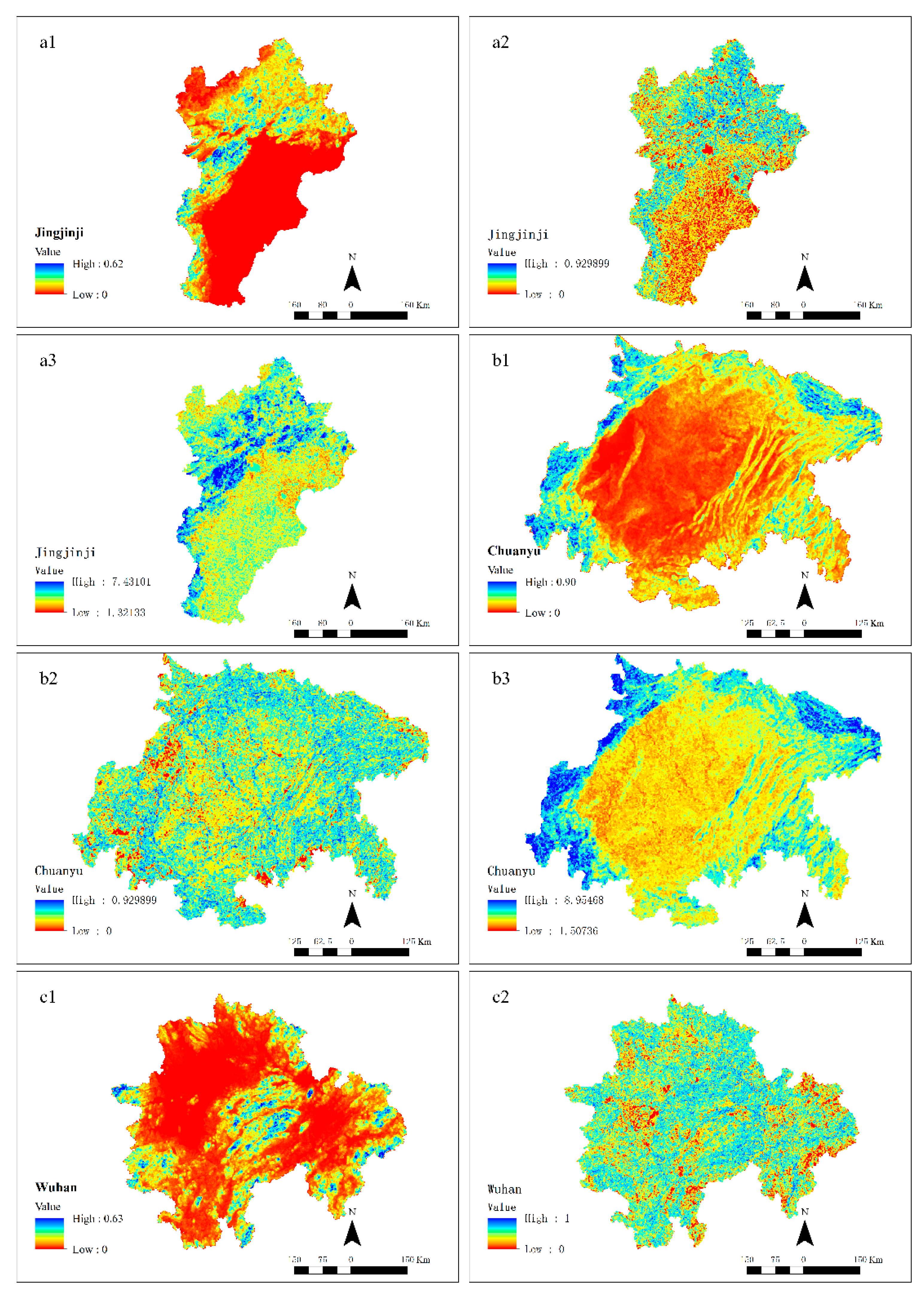
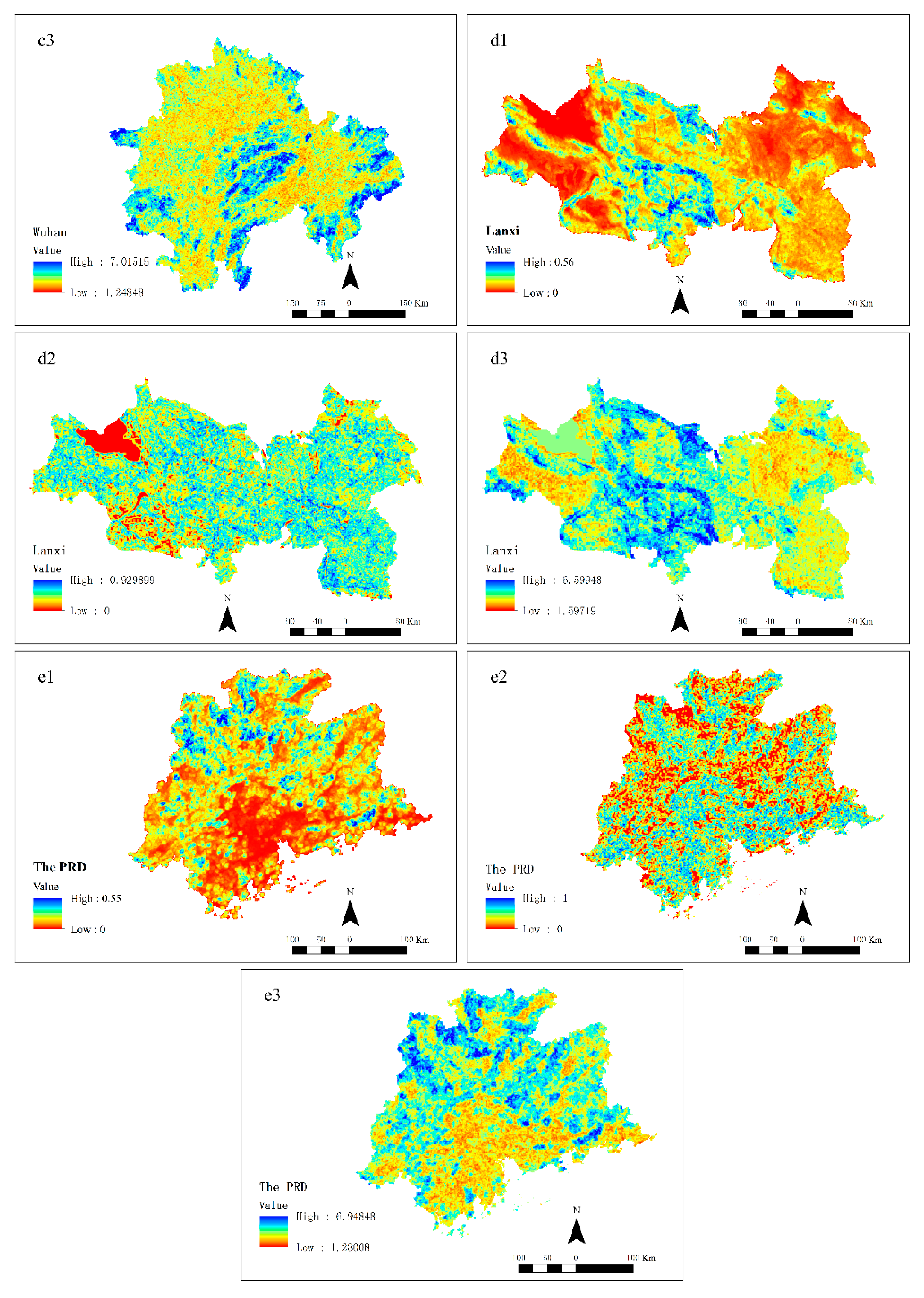
3. Comprehensive Surface Complexity Maps

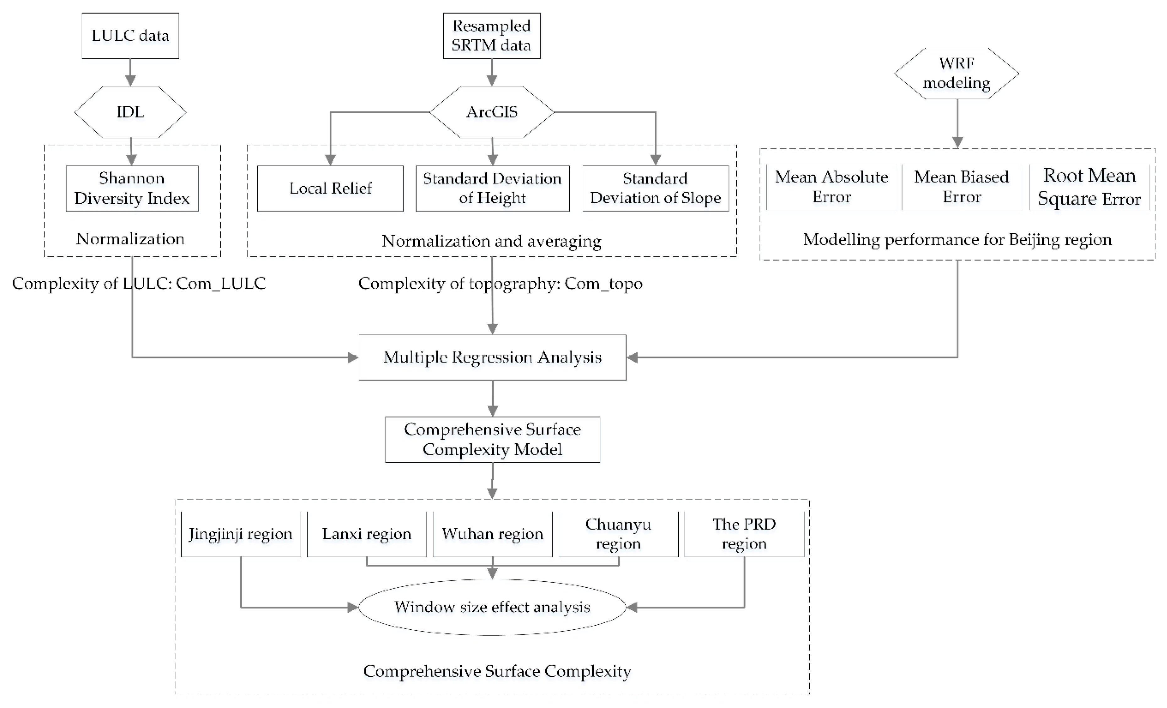
3.1. Research Method

The concept of CSC is proposed to investigate the integrated effect from topography and LULC in geographic process modeling (Figure 3).

To quantify the CSC, Shannon’s diversity index (SHDI), one popular measure of diversity borrowed from community ecology, was employed to quantify the complexity of LULC. The SHDI increases as the number of different LULC types increases and/or the proportional distribution of area among LULC types becomes more equitable. The SHDI equals 0 when the moving window contains only 1 LULC type (i.e., no diversity) and approaches 0 as the distribution of area among the different LULC types becomes increasingly uneven (i.e., dominated by 1 type); and the SHDI equals 1 when the distribution of area among LULC types is perfectly even (i.e., proportional abundances are the same). For the complexity of topography, this study utilizes the local relief (LR), standard deviation of height (SDH), and standard deviation of slope (SDS) to portray the multiple aspects of the complexity. The equations for both LULC and topography are listed in

Table 1. Surface complexity metrics for land use and land cover (LULC) and topography.

Descriptor/Metric	Equation	Parameters	Range
Shannon’s diversity index (SHDI)	$H^{\prime }=-\sum (Pi)(\ln Pi)$	$P_i$= proportion of the landscape occupied by LULC type i.	SHDI ≥ 0, without limit
Local relief (LR)	$\Delta H=H\max -H\min$	H is the height of any point in a moving window	LR ≥ 0, without limit
Standard deviation of height (SDH)	$\sigma =\sqrt{\frac{{\displaystyle \sum _{i=1}^N{(Hi-\overline{H})}^2}}{N-1}}$	$H_i$ is the height of any point in a moving window and N is the number of points in a moving window	SDH ≥ 0, without limit
Standard deviation of slope (SDS)	$\alpha =\sqrt{\frac{{\displaystyle \sum _{i=1}^N{(\theta i-\overline{\theta })}^2}}{N-1}}$	${\theta }_i$ is the slope of any point in a moving window and N is the number of points in a moving window	SDS ≥ 0, without limit

.

The values of each equation in Table 1 are calculated in a moving window over the LULC and DEM data, where the values are reported in the central cell. Among them, the SDS value is based on the slope map, which is calculated first based on the DEM data. The main steps to compute these values are shown in Figure 4, where we implement the interactive data language (IDL) for the LULC complexity index and in ArcGIS 10.2 for the topographic complexity index. To make the values of these indices on different scales compatible with a notionally common scale, normalization concerning all the five study regions is applied prior to finding the weighted average. The normalization method is that the value of each cell is divided by the max value of all the five regions.

To construct the model for CSC, this paper applies the multiple regression analysis method based on the complexity of LULC and topography and the station-based modeling performance in the Beijing region (Figure 5). Based on the observation from each station (an hourly series) with coordinates, we extracted the simulation results from the Weather Research and Forecasting Model (WRF). Then, the mean absolute error (MAE), mean biased error (MBE), and the root mean square error (RMSE) are considered to quantify the modeling performance from WRF [18].

The modeling is run for July 2012; the detailed experiment setup and modeling results are illustrated in [23]. Based on the coordinates of these stations, we extracted the SHDI and complexity of topography with the moving window size of 3 × 3 km which is computed as the mean of the LR, SDH and SDS. For 2 m temperature, one typical meteorological variable, we get the regression between MAE, MBE, and RMSE and the complexity of topography and LULC (

Table 2. Multiple regression analysis for CSC model.

	MAE	MBE	RMSE
Intercept	3.15	3.15	3.56
Complexity of LULC	−1.99	−2.37	−1.78
Complexity of topography	6.88	7.09	7.13
Multiple R	0.45	0.43	0.46

). So in each regression, the MAE, MBE, and RMSE are the dependent variables. The regression model is shown in Equation (1). It can be seen that the Multiple R is approximately 0.45, and the CSC is negatively correlated with the SHDI, positively correlated with the complexity of topography, and generally stable for the AME, ME, and RMSE. Thus, this paper applies the MAE in the CSC model, which is shown in Equation (1). By such regression model, we get the relationship between modeling performance and the surface complexity.

$$\mathrm{CSC}=3.15-1.99\ast SHD{I}_{normalization}+6.88\ast \frac{1}{3}\ast \left(L{R}_{normalization}+SD{H}_{normalization}+SD{S}_{normalization}\right)$$

(1)

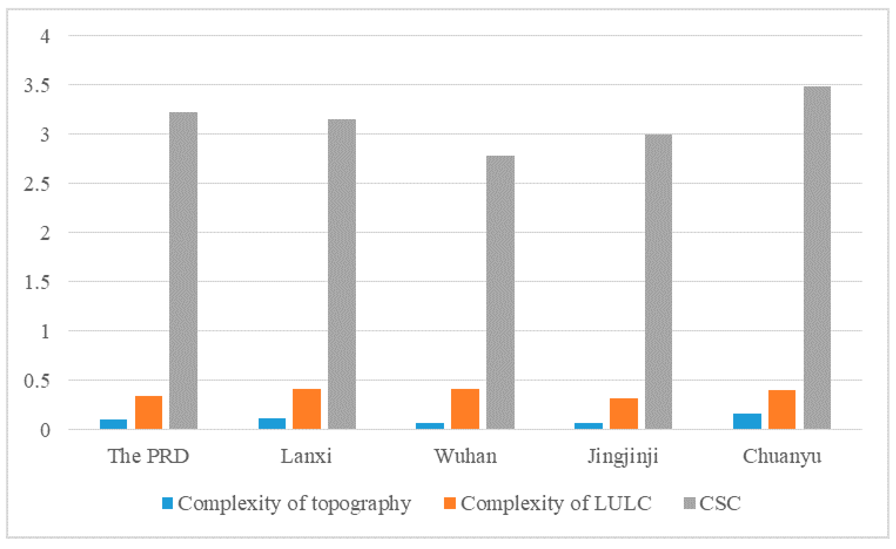
3.2. CSC Metrics and Analysis

3.2.1. CSC Metrics

Based on the CSC model, the LULC, topographic complexity, and CSC maps with moving window size of 3 × 3 km are shown in Figure 6. Along with the data from Figure 7, it can be seen that both the Chuanyu and Lanxi regions have relatively high CSC. Referring to the geographic location from Figure 1, we can see that these two regions are located in the western part of China with high and complex topography. However, the Jingjinji region is of the lowest CSC, which indicates that the ground surface is relatively simple. In addition to the comparison among the different regions concerning the mean value of CSC, the spatial heterogeneity is still obvious in all the study areas from Figure 6.

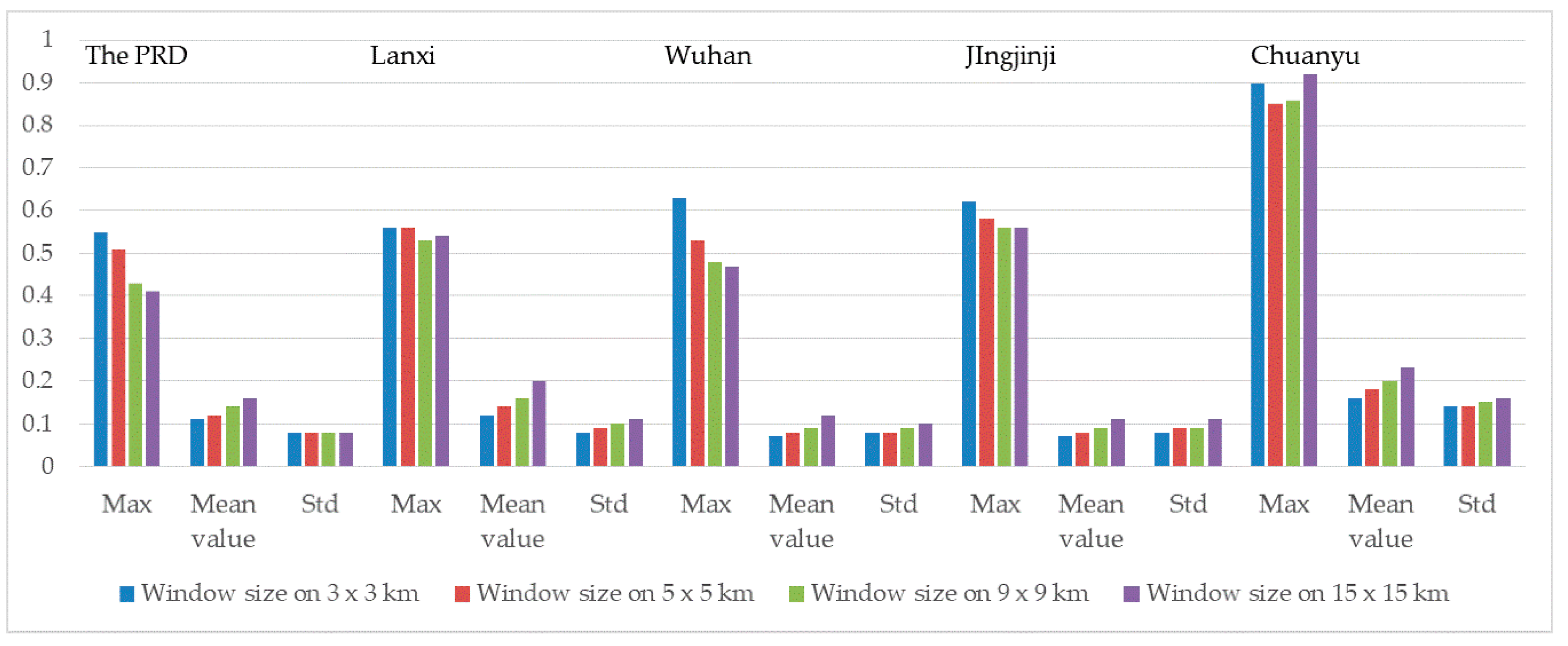
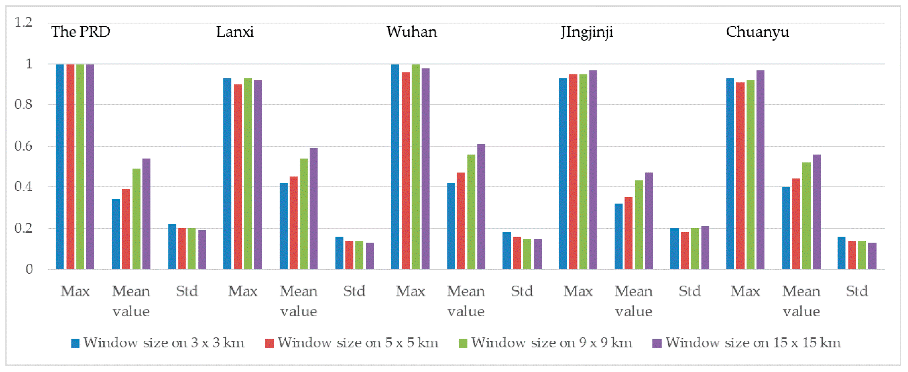
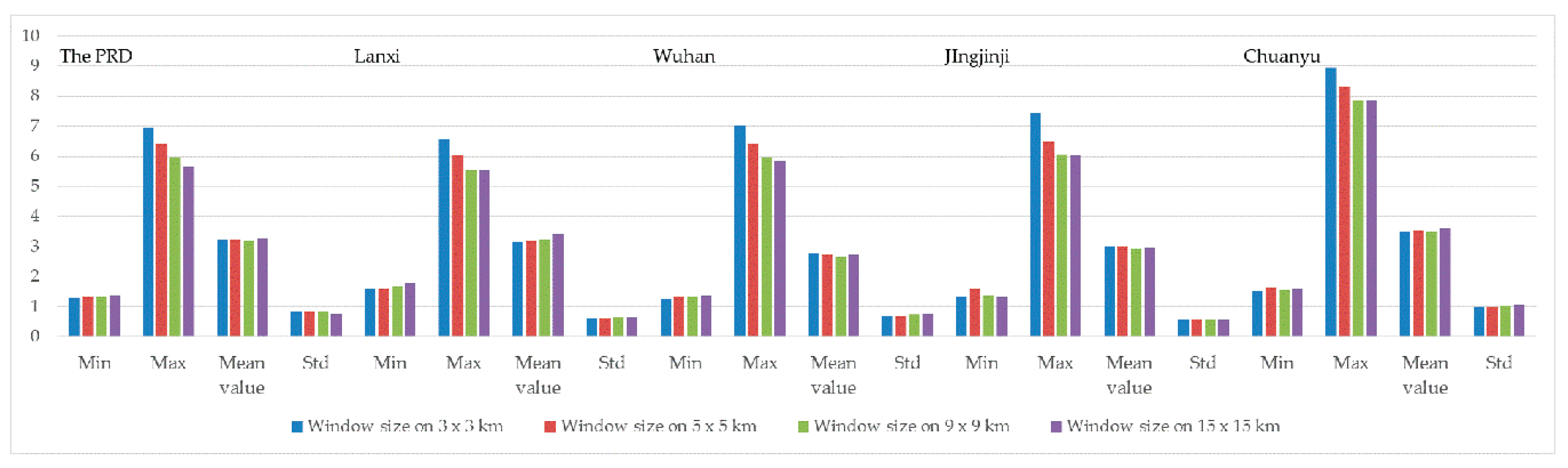
3.2.2. Window Size Effect Analysis

Since CSC is scale dependent like other ground surface indices [24], for values of each equation in Table 1, the width of the moving window varied between 3 and 15 km for each region. Figure 8, Figure 9 and Figure 10 show the statistical values of the complexity of topography and LULC and CSC computed for the five study areas (Figure 1). All the values from different window sizes seem to provide similar results. In detail, the mean and minimum values of CSC increase slightly, and the maximum and standard deviation values decrease or remain the same with the increase in window size. Furthermore, concerning the difference from the five study regions, Jingjinji is of the lowest CSC but has the highest standard deviation. This result means that CSC in this region is more spatially heterogeneous. Based on such analysis, the results from the window size on 3 × 3 km comprehensively describe the complexity of the ground surface.

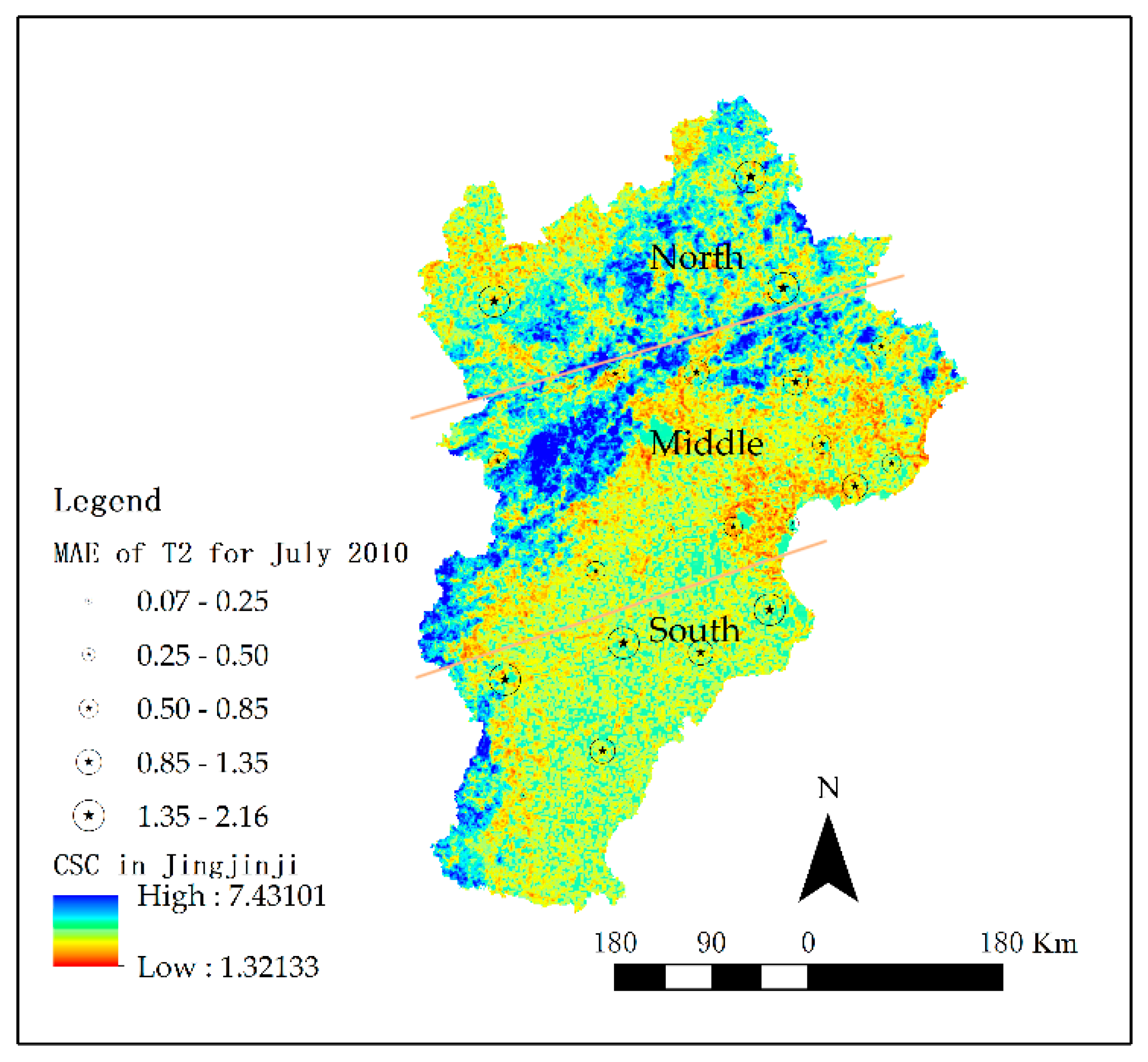
4. Application of CSC in Meteorological Modeling

With geographic data to express the ground surface characters, the WRF model is widely applied to simulate the meteorological situation on the mesoscale. Despite the acknowledged performance, in each simulation domain the modeling accuracy is always spatially heterogeneous. Liu et al. [25] conducted six simulation scenarios with different parameters, but the modeling result is always poor for the site of Shijingshan in Beijing. This result may be affected by the poor expression of the status of topography and LULC [26]. As mentioned in Section 3, the Jingjinji region has a relatively lower mean value of CSC but a higher standard deviation of CSC. We use the Jingjinji region as an example to study the relationship between the heterogeneity of temperature at a 2 meter (T2) modeling performance and the feature of ground surface, which is expressed by CSC.

In this study, we use WRF 3.5 to simulate the meteorology in the Jingjinji region for July 2010. In addition to the U.S. Geological Survey (USGS), topographic and LULC data are preprocessed and reclassified to make the data compatible with the WRF. The T2 accuracy of the WRF simulation is verified by observational data from the Meteorological Data Center at the China Meteorological Administration. The MAE of T2 was applied to describe the modeling performance. For detailed information concerning modeling setup and validation, please refer to Li et al. [19].

The CSC and the MAE of T2 expressed as the size of circle around each station are shown in Figure 11. From the figure, we can see that the MAE is higher over the northern and southern areas and lower over the central part of the study area, which is generally relevant to the value of CSC. Thus, it is feasible to suggest that CSC is helpful to indicate the meteorological modeling capacity and identify those areas where finer scale modeling is preferable.

5. Discussion and Conclusions

5.1. Discussion

1. Complexity and roughness

For topography, complexity is usually identical to roughness. However, for LULC, these two terms are different in research. In this work, the complexity is defined to describe the degree of complexity in spatial patterns of LULC patches in a specific window. Therefore, in this paper, we utilize the landscape index to compute the complexity to LULC.

2. Multiple regression model of CSC

In this work, we compute the CSC by a multiple regression model between meteorological modeling performance and the topographic index and landscape index. The regression parameters show that meteorological modeling performance is quantitatively relevant to surface characteristics, although Multiple R is low. Meteorological modeling performance may be affected by many factors, such as boundary and initial conditions, modeling physical setting, and so on. Surface condition is just one factor, so Multiple R may be low. However, the parameters of such model may still be improved by more observations or evaluation from other regions. However, the application of CSC computed here is favorable concerning the positive relationship in the Jingjinji region. Thus, for more detailed applications on different study regions, the model can be refined accordingly. Furthermore, different index may also be considered to quantify the complexity of topography and LULC [27,28].

3. Concept of CSC

This work is valuable concerning the new concept of CSC, which is a new perspective to forecast and explain the performance of geographic process modeling from the ground surface. The research method used in this paper can be extended to other geographic process modeling in addition to meteorological processes. For instance, concerning the surface hydrological process, surface variables, such as topography, LULC type, and soil type, can be comprehensively considered to quantify the CSC to facilitate process modeling. Meanwhile, the specific parameters in the multiple regression model of CSC for different processes may also vary accordingly, which deserves more evaluation in practice.

5.2. Conclusions

In regard to the close relationship between surface complexity and the performance of geographic process modeling, this paper proposed the concept of CSC, which was quantified comprehensively based on topographic and LULC data. Such CSC is helpful in geographic modeling concerning two aspects. On the one hand, for multiscale modeling, those areas with higher CSC are preferable to set finer scale modeling and vice versa. On the other hand, those areas with higher CSC are usually of relatively poor modeling performance in one modeling domain, which deserves our focused attention.

This paper applied the topographic index and the landscape index to compute the CSC. Based on the multiple regression model between these indices and the modeling performance, we constructed the CSC model and computed the CSC for the five study areas. For the CSC in different study regions, the Chuanyu region had the highest CSC and Wuhan region had the lowest CSC, which gives the indication that for meteorological modeling, it is better to apply a finer setting of modeling for the Chuanyu region in regard to the characteristics of ground surface.

The scale effect concerning the moving window size was also discussed. Based on the window size on 3 × 3, 5 × 5, 9 × 9, and 15 × 15 km, we found an increasing trend for the mean and minimum values of CSC, and nearly decreasing trend for the maximum and standard deviation values along with the increase in window size.

To evaluate the capacity of CSC in indicating the modeling performance, we analyzed the relationship between the CSC and modeling performance of T2 from the WRF model in the Jingjinji region. The result qualitatively showed the positive relationship. In detail, the north and south part is of high CSC with relatively worse modeling performance, and the middle part is of relatively low CSC with better modeling performance.

References

1. Smith, M.W. Roughness in the Earth Sciences. Earth Sci. Rev. 2014, 136, 202–225. [Google Scholar] [CrossRef]
2. Berti, M.; Corsini, A.; Daehne, A. Comparative analysis of surface roughness algorithms for the identification of active landslides. Geomorphology 2013, 182, 1–18. [Google Scholar] [CrossRef]
3. Baldo, E.; Margulis, S.A. Assessment of a multiresolution snow reanalysis framework: A multidecadal reanalysis case over the upper Yampa River basin, Colorado. Hydrol. Earth Syst. Sci. 2018, 22, 3575–3587. [Google Scholar] [CrossRef]
4. Cao, M.; Zhu, Y.; Quan, J.; Zhou, S.; Lü, G.; Chen, M.; Huang, M. Spatial sequential modeling and predication of global land use and land cover changes by integrating a global change assessment model and cellular automata. Earth’s Future 2019. [Google Scholar] [CrossRef]
5. Cao, M.; Huang, M.; Xu, R.; Lü, G.; Chen, M. A grey wolf optimizer–cellular automata integrated model for urban growth simulation and optimization. Trans. GIS. 2019. [Google Scholar] [CrossRef]
6. Mukherjee, S.; Mukherjee, S.; Garg, R.D.; Bhardwaj, A.; Raju, P.L.N. Evaluation of topographic index in relation to terrain roughness and DEM grid spacing. J. Earth Syst. Sci. 2013, 122, 869–886. [Google Scholar] [CrossRef] [Green Version]
7. Li, C.; Wang, Q.; Shi, W.; Zhao, S. Uncertainty modelling and analysis of volume calculations based on a regular grid digital elevation model (DEM). Comput. Geosci. 2018, 114, 117–129. [Google Scholar] [CrossRef]
8. Carvalho, J.C.; Anfossi, D.; Castelli, S.T.; Degrazia, G.A. Application of a model system for the study of transport and diffusion in complex terrain to the TRACT experiment. Atmos. Environ. 2002, 36, 1147–1161. [Google Scholar] [CrossRef]
9. Simova, P.; Gdulova, K. Landscape indices behavior: A review of scale effects. Appl. Geogr. 2012, 34, 385–394. [Google Scholar] [CrossRef]
10. Zhai, Y.; Qu, Z.; Hao, L. Land Cover Classification Using Integrated Spectral, Temporal, and Spatial Features Derived from Remotely Sensed Images. Remote Sens. 2018, 10, 383. [Google Scholar] [CrossRef]
11. Cao, M.; Zhu, Y.; Lü, G.; Chen, M.; Qiao, W. Spatial distribution of global cultivated land and its variation between 2000 and 2010, from both agro-ecological and geopolitical perspectives. Sustainability 2019, 11, 1242. [Google Scholar] [CrossRef]
12. Zhao, C.; Sander, H.A. Assessing the sensitivity of urban ecosystem service maps to input spatial data resolution and method choice. Landsc. Urban Plan. 2018, 175, 11–22. [Google Scholar] [CrossRef]
13. Miller, J.D.; Brewer, T. Refining flood estimation in urbanized catchments using landscape metrics. Landsc. Urban Plan. 2018, 175, 34–49. [Google Scholar] [CrossRef] [Green Version]
14. Zhang, C.; Chen, M.; Li, R.; Fang, C.; Lin, H. What’s going on about geo-process modeling in virtual geographic environments. Ecol. Model. 2016, 319, 147–154. [Google Scholar] [CrossRef]
15. Lü, G.; Batty, M.; Strobl, J.; Lin, H.; Zhu, A.X.; Chen, M. Reflections and speculations on the progress in Geographic Information Systems (GIS): A geographic perspective. Int. J. Geogr. Inf. Sci. 2019, 33, 346–367. [Google Scholar] [CrossRef]
16. Goodchild, M.F. Scale in GIS: An overview. Geomorphology 2011, 130, 5–9. [Google Scholar] [CrossRef]
17. Zhang, C.; Lin, H.; Chen, M.; Li, R.; Zeng, Z. Scale compatibility analysis in geographic process research: A case study of a meteorological simulation in Hong Kong. Appl. Geogr. 2014, 52, 135–143. [Google Scholar] [CrossRef]
18. Zhang, C.; Lin, H.; Chen, M.; Yang, L. Scale matching of multiscale digital elevation model (DEM) data and the Weather Research and Forecasting (WRF) model: A case study of meteorological simulation in Hong Kong. Arab. J. Geosci. 2014, 7, 2215–2223. [Google Scholar] [CrossRef]
19. Li, J.; Zheng, X.; Zhang, C.; Chen, Y. Impact of Land-Use and Land-Cover Change on Meteorology in the Beijing–Tianjin–Hebei Region from 1990 to 2010. Sustainability 2018, 10, 176. [Google Scholar] [CrossRef]
20. Peng, J.; Ma, J.; Liu, Q.; Liu, Y.; Li, Y.; Yue, Y. Spatial-temporal change of land surface temperature across 285 cities in China: An urban-rural contrast perspective. Sci. Total Environ. 2018, 635, 487–497. [Google Scholar] [CrossRef]
21. CGIAR-CSI. SRTM 90m Digital Elevation Data. 2012. Available online: http://srtm.csi.cgiar.org/index.asp (accessed on 21 August 2012).
22. Liu, J.; Kuang, W.; Zhang, Z.; Xu, X.; Qin, Y.; Ning, J.; Wan, C.; Zhou, S.W.; Zhang, R.D.; Li, C.Z.; et al. Spatiotemporal characteristics, patterns, and causes of land-use changes in China since the late 1980s. J. Geogr. Sci. 2014, 24, 195–210. [Google Scholar] [CrossRef]
23. Wang, J.; Feng, J.; Yan, Z. Potential sensitivity of warm season precipitation to urbanization extents: Modeling study in Beijing-Tianjin-Hebei urban agglomeration in China. J. Geophys. Res. Atmos. 2015, 120, 9408–9425. [Google Scholar] [CrossRef]
24. Lane, S.N. Roughness-time for a re-evaluation? Earth Surf. Process. Landf. 2005, 30, 251–253. [Google Scholar] [CrossRef]
25. Liu, R.; Han, Z.; Wu, J.; Hu, Y.; Li, J. The impacts of urban surface characteristics on radiation balance and meteorological variables in the boundary layer around Beijing in summertime. Atmos. Res. 2017, 197, 167–176. [Google Scholar] [CrossRef]
26. Muro, J.; Strauch, A.; Heinemann, S.; Steinbach, S.; Thonfeld, F.; Waske, B.; Diekkrüger, B. Land surface temperature trends as indicator of land use changes in wetlands. Int. J. Appl. Earth Obs. Geoinf. 2018, 70, 62–71. [Google Scholar] [CrossRef]
27. Abrantes, P.; Rocha, J.; Marques da Costa, E.; Gomes, E.; Morgado, P.; Costa, N. Modelling urban form: A multidimensional typology of urban occupation for spatial analysis. Environ. Plan. B Urban Anal. City Sci. 2017, 46, 1–19. [Google Scholar] [CrossRef]
28. Almeida, D.; Rocha, J.; Neto, C.; Arsénio, P. Landscape metrics applied to formerly reclaimed saltmarshes: A tool to evaluate ecosystem services? Estuar. Coast. Shelf Sci. 2016, 181, 100–113. [Google Scholar] [CrossRef]
Figure 1. Location map of the study areas with elevation.
Sustainability 11 04081 g001
Figure 2. Land use and land cover of the study areas.
Sustainability 11 04081 g002
Figure 3. Definitions of comprehensive surface complexity.
Sustainability 11 04081 g003
Figure 4. Main steps used in computing the comprehensive surface complexity (CSC) for the study areas.
Sustainability 11 04081 g004
Figure 5. Station based observations for multiple regression analysis to construct the CSC model.
Sustainability 11 04081 g005
Figure 6. Complexity maps for the study areas. For each region, in the Figure 6, (a1e1) are for the complexity of LULC, (a2e2) are for the topographic complexity, and (a3e3) are for the CSC maps.
Sustainability 11 04081 g006aSustainability 11 04081 g006b
Figure 7. Average complexity values for each study area.
Sustainability 11 04081 g007
Figure 8. Window size effect analysis of the complexity of topography.
Sustainability 11 04081 g008
Figure 9. Window size effect analysis of the complexity of LULC.
Sustainability 11 04081 g009
Figure 10. Window size effect analysis of CSC.
Sustainability 11 04081 g010
Figure 11. Map of observation stations and CSC of the Jingjinji region, with the size of circles indicating the value of mean absolute error (MAE).
Sustainability 11 04081 g011