Do Overnight Returns Truly Measure Firm-Specific Investor Sentiment in the KOSPI Market?

Abstract

This study analyzes the effect of overnight returns on subsequent stock market returns and investigates whether they do capture investor sentiment in the Korean stock market. Recent study showed that overnight returns are similar to existing sentiment measures, and, thus, are suitable for measuring firm-specific investor sentiment in the U.S. market. Similarly, we found that, for firms in the Korean market, high overnight returns are followed by higher stock returns in the short term (i.e., two or three trading days) but lower stock returns in the long term. However, these effects do not differ for different types of firms (i.e., hard-to-value firms), whereas classical firm-specific sentiment indicators capture these differences. Overall, we found that overnight returns do not truly measure firm-specific investor sentiment in the Korean stock market even though they are partially related to investor sentiment.

1. Introduction

Although the classical asset pricing framework, which is based on the concepts of investor rationality, optimization, and market efficiency, governs economic studies, the recent financial crises and episodes of irrational exuberance bring the validity of rational asset pricing models into question. Both academics and market practitioners are beginning to focus on investor irrationality and behavior to explain market anomalies and abnormal asset price movements. As a result, the field of behavioral finance has emerged. Behavioral finance studies, which examine investors’ overreactions, underreactions, disposition effects, noise trading, herding phenomena, moods, and sentiments, empirically analyze both developed (Branch and Evans, 2010 [1]; Devault, Sias, and Starks, 2019 [2]; Kothari, Lewellen, and Warner, 2006 [3]) and emerging (Ryu, 2013 [4]; Shim, Kim, Kim, and Ryu, 2015 [5]; Shim, Kim, and Ryu, 2017 [6]; Yang, Ahn, Kim, and Ryu, 2017 [7]) markets.

In recent studies, academics developed the concept of “investor sentiment” and incorporated this concept into financial and economic models to better explain asset price dynamics (Hwang, 2011 [8]; Li and Luo, 2016 [9]; Yu and Yuan, 2011 [10]). Following the seminal study of Baker and Wurgler (2006) [11], most studies in this field adopted and extended Baker and Wurgler’s (2006) [11] market-wide sentiment indicators (Berger and Turtle, 2015 [12]; Huang, Jiang, Tu, and Zhou, 2015 [13]; Kim, Ryu, and Seo, 2014 [14]; Stambaugh, Yu, and Yuan, 2014 [15]). However, aggregate sentiment indicators in the style of Baker and Wurgler (2006) [11] have some shortcomings in that they do not precisely capture individual firm characteristics and they often lose their explanatory power for stock market returns when macroeconomic variables are considered (Kim and Na, 2018 [16]). Recent studies develop new sentiment indicators for emerging financial markets that capture different firm characteristics and are available at higher frequencies. For example, Yang and Zhou (2015 [17], 2016 [18]) and Yang and Yang (2019 [19]) constructed a measure that describes investor sentiment dynamics at the individual firm level in the Chinese financial market. Ryu, Kim, and Yang (2017 [20]) and Yang, Ryu, and Ryu (2017 [21]) extended these firm-level sentiment indicators to analyze the behavior of the Korean stock market. In these recent studies, the new sentiment measures are called “firm-specific” sentiment indicators.

The applications of these firm-specific sentiment indicators are remarkable. Specifically, using these indicators, Seok, Cho, and Ryu (2019a [22]) found that the sentiment influences the relationship between earnings news and stock market returns. Kim, Ryu, and Yang (2019 [23]) analyzed the associations among analyst recommendation changes, stock returns, and investor sentiment. These recent, innovative studies focus on the role of investor sentiment in explaining market dynamics, which previous studies overlook.

In this study, we validate the effectiveness of firm-specific sentiment indicators and compare them with other candidate indicators of sentiment (i.e., overnight returns) in the Korean market, a representative and leading emerging market (Chung, Cho, Ryu, and Ryu, 2019 [24]; Lee and Ryu, 2019 [25]). This study is also motivated by the importance of the Korean market, as demonstrated by its influence on other emerging markets, its open economy, and its rapidly growing economic power. The importance, influence, openness, and other unique characteristics of the Korean financial market are well documented by previous studies, including those of Chun, Cho, and Ryu (2018) [26]; Chung, Kang, and Ryu (2018) [27]; Lee, Ryu, and Kutan (2016) [28]; Ryu, Ryu, and Hwang (2016 [29], 2017 [30]); and Shim, Kim, and Ryu (2017) [6].

Specifically, we analyze the effect of overnight returns in the Korean Composite Stock Price Index (KOSPI) market by following a similar methodology to that of Aboody, Even-Tov, Lehavy, and Trueman (2018) [31]. We investigate whether overnight returns truly measure investor sentiment and, thus, can replace the existing firm-level sentiment indicators in this market. The KOSPI market is highly dependent on the U.S. (Kim, Ryu, and Seo, 2015 [32]; Kim and Ryu, 2015 [33]; Park, Kutan, and Ryu, 2019 [34]; Song, Park, and Ryu, 2018 [35]; Song, Ryu, and Webb, 2016 [36], 2018 [37]) and other foreign stock markets, and, thus, stock returns when the KOSPI market is closed might meaningfully affect subsequent returns. Overnight returns in the KOSPI market may, therefore, be driven by factors besides investor sentiment, and our results confirm that these returns are only partially related to investor sentiment. Firms with high overnight returns outperform firms with low overnight returns in the short term but underperform them in the long term. This result indicates that overnight returns do measure investor sentiment in the KOSPI market. However, this effect is not stronger for difficult-to-arbitrage firms. For example, large firms and firms with low idiosyncratic volatilities, high profitability levels, and high institutional trade ratios are more affected by overnight returns. This result contradicts those of previous studies of investor sentiment. However, when we control for other pricing factors such as the market, size, value, and momentum, the effects of overnight returns are greater for small firms and for firms with high idiosyncratic volatilities and book-to-market ratios and low institutional trade ratios, that is, difficult-to-arbitrage firms. Thus, although overnight returns are partially related to investor sentiment in the KOSPI market, it is difficult to conclude that they genuinely measure only investor sentiment.

The remainder of this paper is organized as follows. Section 2 reviews the related literature on the sentiment. Section 3 describes the empirical approach, and Section 4 presents the data used in this study. Section 5 presents the empirical results, and Section 6 concludes.

2. Literature Review

This study investigates the relationship between overnight returns and investor sentiment in the KOSPI market. Investor sentiment refers to investors’ beliefs about the stock market’s prospects regardless of its fundamental value. Uninformed investors tend to trade as a group according to each other’s trades, leading to irrational price co-movement. This co-movement is termed investor sentiment. Traditional financial theory denies that sentiment affects the market because it assumes an efficient market and rational investors. Thus, according to these theories, price movement caused by irrational sentiment should be offset by the actions of rational arbitrageurs. However, recent studies found that investor sentiment plays a vital role in stock market mispricing, especially when arbitrage opportunities are limited.

Early studies in this field attempted to model investor sentiment (Barberis, Shleifer, and Vishny, 1998 [38]; Campbell and Kyle, 1993 [39]), but noise is hard to measure directly, thus researchers try to use market co-movement as a proxy for the sentiment. For example, Lee, Shleifer, and Thaler (1991) [40] and Ben-Rephael, Kandel, and Wohl (2012) [41] used discounts on closed-end funds and mutual fund flow, respectively, to measure sentiment. Fisher and Statman (2003) [42] and Schmeling (2009) [43] used the consumer confidence level to measure sentiment, and Yang and Zhang (2014) [44] tried to measure sentiment using the turnover rate. Also, researchers used various proxies for sentiments, such as market liquidity, IPO data, trading volumes, and news or Twitter data (Baker and Stein, 2004 [45]; Dorn, 2009 [46]; Da, Engelberg, and Gao, 2015 [47]; Liao, Huang and Wu, 2011 [48]). Using these proxies, previous studies estimated the effect of sentiment on subsequent stock returns (Baker and Wurgler, 2006 [11]; Bathia and Bredin, 2013 [49]; Corredor, Ferrer, and Santamaria, 2013 [50]; Gao and Yang, 2017 [51]; Mangee, 2017 [52]; Ryu, Kim, and Yang, 2017 [20]; Schmeling, 2009 [43]; Yang, Ryu, and Ryu, 2017 [21]). In particular, Baker and Wurgler (2006) [11] measured market-wide investor sentiment using a principal component analysis of sentiment proxies (i.e., closed-end fund discounts, the turnover ratio, the number of initial public offerings (IPOs), the first-day returns of IPOs, dividend premiums, and the share of total equity and debt issues that are equity issues). They found that periods of high sentiment are followed by low stock returns on a yearly or monthly basis as the overpricing caused by sentiment is corrected. They also showed that this effect is stronger for difficult-to-arbitrage firms—that is, small, young, highly volatile, or unprofitable firms. Baker, Wurgler, and Yuan (2012) [53] expanded this analysis to a global sample and found similar results, and Brzeszczynski, Gajdka, and Kutan (2015) [54], Chen and Lien (2017) [55], and Seok, Cho, and Ryu (2019a) [22] investigated the relationship between sentiment and news and found that investors react more strongly to good news when sentiment is high.

One disadvantage of these sentiment measures is that they are market-wide measures. Investor sentiment should differ across firms; thus, Ryu, Kim, and Yang (2017 [20]), Seok, Cho, and Ryu (2019a [22]), and Yang and Zhou (2015 [17], 2016 [18]) tried to measure firm-specific investor sentiment using high-frequency data such as price and trading volume data. These studies considered the relationship between sentiment and short-term returns. They found that the mispricing caused by investor sentiment is not immediately corrected, but rather lasts for two or three trading days, for example. As a result, firms with high investor sentiment have higher stock returns in the short term, and this effect is stronger for difficult-to-arbitrage firms. Additionally, Aboody, Even-Tov, Lehavy, and Trueman (2018) [31] investigated overnight returns in the U.S. stock market and argued that such returns effectively measure firm-specific investor sentiment. They showed that overnight returns exhibit short-term persistence and that this persistence is stronger for difficult-to-arbitrage firms. Furthermore, they found that firms with high overnight returns underperform other firms in the long term.

3. Methodology

To investigate whether overnight stock returns indeed reflect firm-specific investor sentiment, we adopt two primary methodologies. The first methodology comes from Seok, Cho, and Ryu (2019a [22], 2019b [56]), and the second comes from Baker and Wurgler (2006) [11]. Specifically, we first analyze daily stock returns based on overnight returns. Many previous studies show that high investor sentiment causes overpriced stocks, and, thus, firms with high investor sentiment later experience lower stock returns over subsequent months or years as the overpricing is corrected (Baker and Wurgler, 2006 [11]; Baker, Wurgler, and Yuan, 2012 [53]; Schmeling, 2009 [43]). Recent studies analyzed daily investor sentiment and showed that mispricing caused by investor sentiment is not immediately corrected but rather persists for at least one to three days. Thus, firms with high investor sentiment experience higher stock returns in the short term, but these returns decrease after a few days as the mispricing is corrected (Yang, Ryu, and Ryu, 2018 [57]; Yang and Zhou, 2015 [17], 2016 [18]). Thus, if overnight returns truly measure firm-specific investor sentiment, firms with high overnight returns should have higher short-term stock returns that decrease after a few days. To confirm this hypothesis, we use Fama–MacBeth regressions to analyze long–short portfolio returns for portfolios formed based on overnight returns. Fama–MacBeth regressions estimate the parameters of asset pricing models and, thus, we can use this regression method to analyze whether overnight returns significantly affect subsequent returns. Moreover, Fama–MacBeth regressions have the advantage of working well with multiple assets across time (i.e., panel data). Thus, they are widely used to analyze asset pricing or portfolio returns and are appropriate for analyzing the pricing effects of specific factors such as sentiment. Ryu, Kim, and Yang (2017 [20]) and Seok, Cho, and Ryu (2019b) [56] investigated the effect of sentiment on corresponding stock returns using this methodology. Equation (1) shows the detailed methodology.

$$\begin{array}{c}Re{t}_{i,t+k}={\alpha }_i+{\beta }_{\mathrm{i}}\times Ove.Re{t}_{i,t}+{\beta }_{i,MKT}\times MK{T}_{t+k}+{\beta }_{i,SMB}\times SM{B}_{t+k}+\\ {\beta }_{i,HML}\times HM{L}_{t+k}+{\beta }_{i,UMD}\times UM{D}_{t+k}+{\epsilon }_{i,t+k},\end{array}$$

(1)

Here, Ret_i,t+k denotes firm i’s return on day t+k; Ove.Ret_i,t denotes firm i’s overnight return on day t; and MKT_t+k, SMB_t+k, HML_t+k, and UMD_t+k are Carhart’s [58] four factors on day t+k. Specifically, MKT is the excess market (i.e., KOSPI) return over the risk-free rate (i.e., the 91-day certificate of deposit rate); SMB is the difference between the returns to small and large portfolios; HML is the difference between the returns to high and low BE/ME portfolios; and UMD is the difference between the returns to high-momentum and low-momentum portfolios, where momentum is measured from month t – 12 to month t – 2. We expect that the coefficient of the overnight return, β_i, is positive in the short term but negative in the long term, as is the case for other sentiment measures (Seok, Cho, and Ryu, 2019a [22], 2019b [56]).

The second methodology used in this study is that of Baker and Wurgler (2006) [11]. They showed that the effect of sentiment is stronger for difficult-to-arbitrage firms using a sorting test and long–short portfolio regressions on sentiment, where portfolios are formed based on firm characteristics. Aboody, Even-Tov, Lehavy, and Trueman (2018) [31] and Shen, Yu, and Zhao (2017) [59] also used sorting and long–short portfolio tests and found similar results to those of Baker and Wurgler (2006) [11]. Thus, we use these methodologies to investigate whether the effects of overnight returns are more prominent for difficult-to-arbitrage firms. More specifically, we create ten value-weighted portfolios based on firm characteristics at each quarter end and calculate the value-weighted and overnight returns for each portfolio. Then, we divide the full sample period into periods of high and low overnight returns (i.e., above and below the median, respectively) for each portfolio and also analyze the next-day returns of each portfolio. We also analyze the differences between the returns in high and low periods. Then, we construct a long–short portfolio based on firm characteristics and analyze the effect of overnight returns on the returns to this long–short portfolio.

4. Empirical Data

In this study, we analyze Korean manufacturing firms listed on the KOSPI market. We exclude data from the day before the beginning of the suspension to the day after the end of the suspension to avoid data-related issues. We ultimately analyze 152,909 daily returns for 451 manufacturing firms from January 2001 to October 2018. We measure each firm’s overnight return as the difference between its opening price on the current day and its closing price on the previous operating day divided by its closing price on the previous operating day. Here, we use the adjusted share price to avoid any sharp decreases or increases in stock prices due to rights issues or stock splits. The stock price data come from the FnGuide database. Equation (2) shows the full expression for a firm’s overnight return.

$$Overnigh{t}_{i,t}=\frac{Openin{g}_{i,t}-Closin{g}_{i,t-1}}{Closin{g}_{i,t-1}},$$

(2)

where Opening_i,t is the adjusted opening price for firm i on day t and Closing_i,t−1 is the adjusted closing price for firm i on day t − 1.

We use quarterly data to measure firm characteristics such as size, idiosyncratic volatility, profitability, book-to-market ratio, leverage, and the institutional trading ratio. These variables are constructed following Seok, Cho, and Ryu’s (2019b [56]) methodology, and we obtain 25,493 quarterly observations for the firm-characteristic variables. Firm size (i.e., ME) is measured as the product of outstanding shares and the closing price at the end of the quarter. Smaller firms are harder to value and, thus, should be more affected by investor sentiment (Baker and Wurgler, 2006 [11]). Small firms should, therefore, be more affected by overnight returns if overnight returns measure investor sentiment (Aboody, Even-Tov, Lehavy, and Trueman, 2018 [31]). Idiosyncratic volatility (i.e., IVOL) is calculated as the standard deviation of the residuals of Carhart’s four-factor model. IVOL reflects risk, which deters arbitrage (Stambaugh, Yu, and Yuan, 2014 [15]) and, thus, firms with high IVOL are more influenced by investor sentiment (Seok, Cho, and Ryu, 2019b [56]). The book-to-market ratio (i.e., BE/ME) represents a firm’s opportunity for growth and is measured as shareholder equity divided by firm size at quarter end. Seok, Cho, and Ryu (2019b [56]) argued that firms with high book-to-market ratios have greater opportunity for growth and, thus, are harder to value and more affected by investor sentiment in the KOSPI market. E/BE, which represents net earnings divided by shareholder equity, and D/E, which represents total debt divided by total equity, capture a firm’s profitability and financial distress, respectively. Baker and Wurgler (2006) [11] showed that less profitable firms and firms with higher financial distress are more affected by investor sentiment. Finally, the institutional trade ratio (i.e., Inst), directly captures the ease of arbitrage. Because institutional traders are considered arbitrage traders, a higher institutional trade ratio implies that more arbitrage traders trade that firm’s stock. We calculate the institutional trade ratio as the sum of a stocks’ institutional sales and purchases divided by its total sales and purchases.

Table 1. Summary statistics of firm-characteristic variables.

	N	Mean	SD	Min	Max
Panel A. Stock Returns and Sentiment for Individual Firms (Daily Data)
Return (%)	1,562,909	0.08	3.17	−30.00	30.00
Overnight (%)	1,562,909	0.07	1.83	−30.00	30.00
Panel B. Firm Characteristics (Quarterly Data)
Ln (ME)	25,493	25.56	1.69	21.70	31.73
IVOL (%)	25,493	2.49	1.25	0.52	9.68
E/BE	25,493	0.02	0.05	−0.61	0.79
BE/ME	25,493	1.62	1.38	−15.11	13.25
D/E	25,493	1.19	1.60	−12.31	39.12
INST	25,493	0.22	0.23	0.00	0.97

shows the summary statistics for each variable, where Panel A summarizes the daily data on stock returns and overnight returns and Panel B summarizes the quarterly data on the firm-characteristic variables. For size, we present the log value of market equity because this variable takes large values. N is the number of observations and Mean and SD denote the average and the standard deviation, respectively. Min indicates minimum values and Max indicates maximum values.

5. Results and Discussion

5.1. Overnight Returns and Individual Stock Returns

Panel A of

Table 2. Overnight returns and short-term stock returns.

Panel A. Fama–MacBeth Regression
	t+1		t+2		t+3		t+4		t+5
Intercept	0.0000	−0.0001	0.0004	0.0002 **	0.0004	0.0002 ***	0.0004	0.0002 ***	0.0004	0.0003 ***
	(−0.19)	(−0.85)	(1.50)	(2.79)	(1.64)	(3.26)	(1.64)	(3.39)	(1.68)	(3.54)
Overnight	0.6280 ***	0.5268 ***	0.0438 ***	0.0368 ***	0.0188 *	0.0116 ***	−0.0043	−0.0032	−0.0184 **	−0.0068 ***
	(46.64)	(18.29)	(4.43)	(9.07)	(1.97)	(3.38)	(−0.42)	(−1.38)	(−2.47)	(−3.58)
MKT		0.7540 ***		0.9340 ***		0.9344 ***		0.9344 ***		0.9347 ***
		(60.71)		(120.29)		(131.90)		(129.70)		(127.52)
SMB		0.5895 ***		0.7139 ***		0.7139 ***		0.7152 ***		0.7154 ***
		(44.98)		(46.21)		(47.08)		(46.48)		(45.80)
HML		0.1456 **		0.1917 ***		0.1930 ***		0.1938 ***		0.1934 ***
		(2.23)		(3.00)		(3.04)		(3.04)		(3.06)
UMD		−0.0136		−0.0357 **		−0.0342 *		−0.0352 *		−0.0351 *
		(−0.62)		(−2.15)		(−2.05)		(−2.11)		(−2.10)
Adj R2	0.1260	0.2052	0.0011	0.1230	0.0007	0.1226	0.0006	0.1225	0.0004	0.1225
Panel B. Long–Short Return
Return	0.0162 ***		0.0009 ***		0.0004 ***		0.0002 **		0.0001 *
	(120.05)		(8.88)		(4.79)		(2.08)		(1.66)
Alpha	0.0158 ***		0.0005 ***		0.0000		−0.0002 **		−0.0002 ***
	(118.91)		(5.64)		(0.27)		(−2.15)		(−2.64)

Notes: ^*, ^**, and ^*** denote statistical significance at the 10, 5, and 1% levels, respectively.

shows the results of estimating Equation (1). The left columns for each value of t+k show the results of univariate regression models that only include overnight returns, and the right columns for each value of t+k show the results of regressions including Carhart’s four factors (MKT, SMB, HML, and UMD). Here, t+k denotes the return after k days. Panel B of Table 2 shows the raw returns and the four-factor alphas resulting from a long–short strategy that buys stocks with high overnight returns and sells stocks with low overnight returns. Here, we define high overnight returns as those in the top three deciles and low overnight returns as those in the bottom three deciles. In Table 2, t-statistics are given in brackets, and the superscripts ^*, ^**, and ^*** denote statistical significance at the 10, 5, and 1% levels, respectively.

Panel A of Table 2 shows that overnight returns positively affect returns the following day. This effect diminishes as time passes but remains positive until three days have passed. However, overnight returns negatively affect returns after five days. This result is similar to those of Seok, Cho, and Ryu (2019b [56]) and other studies that analyze the effect of daily sentiment. The overpricing caused by sentiment is not corrected immediately and, thus, sentiment positively affects returns in the short term. However, the mispricing is eventually corrected after a few days and, thus, stocks with high sentiment have lower returns in the long term. The results in Panel B support the results in Panel A. Specifically, stocks with high overnight returns outperform stocks with low overnight returns in the short term, but this phenomenon is reversed in the long term. In short, the effect of overnight returns on short-term and long-term returns is similar to that of sentiment.

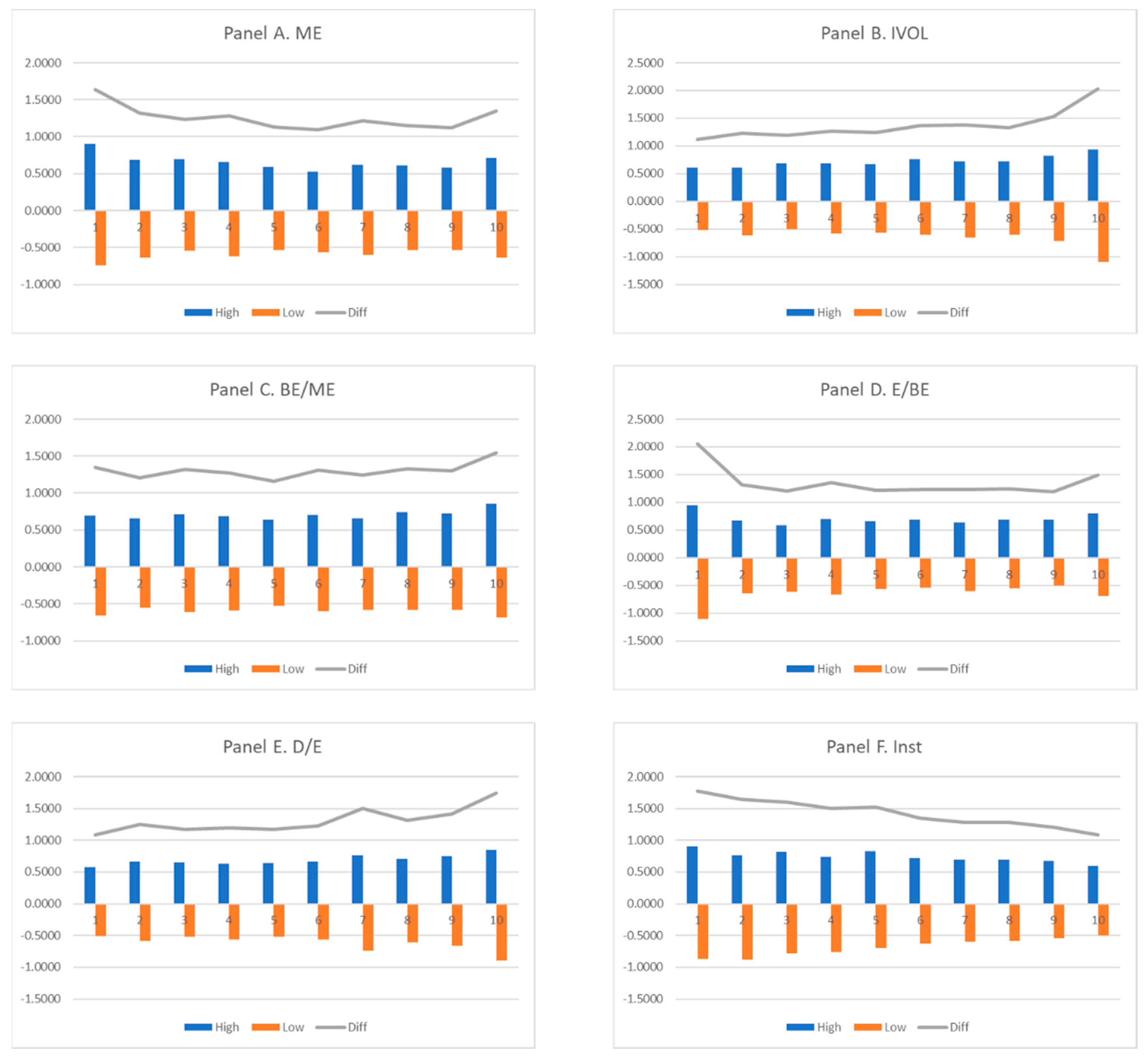
5.2. Individual Stock Returns by Firm Characteristics and Overnight Returns

In this subsection, we investigate whether the effect of overnight returns differs according to firm characteristics.

Table 3. Next-day stock returns sorted by firm characteristics.

		Decile
	Overnight	1	2	3	4	5	6	7	8	9	10
ME	High (%)	0.897	0.685	0.690	0.661	0.594	0.530	0.616	0.612	0.586	0.712
	Low (%)	−0.739	−0.636	−0.542	−0.624	−0.537	−0.561	−0.604	−0.534	−0.538	−0.641
	Difference (%)	1.640	1.320	1.230	1.280	1.130	1.090	1.220	1.150	1.120	1.350
IVOL	High (%)	0.604	0.613	0.681	0.681	0.672	0.761	0.724	0.722	0.819	0.938
	Low (%)	−0.513	−0.620	−0.506	−0.585	−0.564	−0.606	−0.652	−0.608	−0.714	−1.090
	Difference (%)	1.120	1.230	1.190	1.270	1.240	1.370	1.380	1.330	1.530	2.030
BE/ME	High (%)	0.698	0.659	0.713	0.681	0.635	0.705	0.655	0.745	0.720	0.858
	Low (%)	−0.655	−0.555	−0.607	−0.592	−0.529	−0.604	−0.581	−0.586	−0.585	−0.685
	Difference (%)	1.350	1.210	1.320	1.270	1.160	1.310	1.240	1.330	1.300	1.540
E/BE	High (%)	0.946	0.673	0.588	0.693	0.655	0.684	0.629	0.687	0.681	0.798
	Low (%)	−1.100	−0.644	−0.617	−0.669	−0.568	−0.544	−0.599	−0.555	−0.507	−0.688
	Difference (%)	2.050	1.320	1.200	1.360	1.220	1.230	1.230	1.240	1.190	1.490
D/E	High (%)	0.575	0.665	0.652	0.631	0.644	0.667	0.764	0.703	0.749	0.850
	Low (%)	−0.506	−0.587	−0.523	−0.562	−0.525	−0.567	−0.734	−0.606	−0.664	−0.895
	Difference (%)	1.080	1.250	1.170	1.190	1.170	1.230	1.500	1.310	1.410	1.740
Inst	High (%)	0.899	0.760	0.819	0.736	0.830	0.718	0.691	0.691	0.670	0.593
	Low (%)	−0.872	−0.877	−0.782	−0.764	−0.690	−0.629	−0.591	−0.589	−0.542	−0.496
	Difference (%)	1.770	1.640	1.600	1.500	1.520	1.350	1.280	1.280	1.210	1.090

shows the numerical results of the sorting test described in Section 3. All values in this table are significant at the 1% level. Figure 1 shows the results graphically. The blue bars show daily returns following days with high values of Overnight, and the red bars show daily returns following days with low values of Overnight. The solid lines indicate the differences between these two returns.

The first row of Table 3 and Panel A of Figure 1 show the difference in the effect of overnight returns on next-day returns for firms of different sizes. These results indicate no significant difference in overnight returns according to firm size. Similarly, the third and fourth rows of Table 3 and Panels C and D of Figure 1 show that the effects of overnight returns on next-day returns do not differ for firms with different book-to-market ratios or profitability levels. These results suggest that overnight returns do not adequately capture investor sentiment because the effect of sentiment should be more prominent for harder-to-value firms, that is, small firms, firms with high book-to-market ratios, and unprofitable firms (Baker and Wurgler, 2006 [11]). However, the second, fifth, and sixth rows of Table 3 and Panels B, E, and F of Figure 1 suggest that overnight returns do have a stronger effect for firms with higher idiosyncratic volatilities, higher leverage ratios, and lower institutional trade ratios. These results are similar to those found for the sentiment. Thus, the results in Table 3 and Figure 1 suggest that overnight returns partially capture investor sentiment. However, they do not necessarily imply that overnight returns truly measure investor sentiment because the effect of overnight returns on short-term stock returns does not consistently differ across firms of different sizes, idiosyncratic volatilities, book-to-market ratios, profitability levels, leverage amounts, and institutional trade ratios, all of which capture the ease of arbitrage. One explanation for these inconsistencies may be that the effect differs only for firms that are extremely difficult or extremely easy to arbitrage. To confirm this hypothesis, we divide the sample into two subgroups, one with portfolios in the top three deciles and one with portfolios in the bottom three deciles, and we exclude portfolios in the middle deciles. Then, we measure the overnight returns for each subgroup and separately investigate their effects on short-term returns and the difference in these effects. This analysis can capture differences in the effect of overnight returns for extremely difficult-to-arbitrage and extremely easy-to-arbitrage firms. Equation (3) describes the analysis in detail.

$$\begin{array}{c}Re{t}_{p,t}={\alpha }_p+{\beta }_{\mathrm{p}}\times Ove.Re{t}_{p,t}+{\beta }_{p,MKT}\times MK{T}_t+{\beta }_{p,SMB}\times SM{B}_t+\\ {\beta }_{p,HML}\times HM{L}_t+{\beta }_{p,UMD}\times UM{D}_t+{\epsilon }_{p,t},\end{array}$$

(3)

where Ret_p,t denotes the portfolio return (for portfolios in top three and bottom three deciles) on day t; Ove.Ret_p,t denotes the overnight portfolio return on day t; and MKT_t, SMB_t, HML_t, and UMD_t represent Carhart’s four factors on day t.

Table 4. Time series regressions of portfolio returns on overnight returns according to firm characteristics.

	Sentiment			Sentiment with Carhart’s Four Factors
	High	Low	Diff	High	Low	Diff
ME	0.8311 ***	0.7350 ***	0.0993 ***	0.1853 ***	0.5782 ***	−0.3878 ***
	(42.31)	(30.88)	(2.95)	(12.96)	(25.26)	(−11.71)
IVOL	0.7969 ***	0.8648 ***	−0.0810 **	0.4155 ***	0.1485 ***	0.2575 ***
	(36.36)	(45.01)	(−2.39)	(21.10)	(11.49)	(8.31)
BE/ME	0.8666 ***	0.8303 ***	0.0353	0.5416 ***	0.1840 ***	0.3542 ***
	(39.71)	(42.33)	(1.14)	(27.12)	(13.72)	(12.78)
E/BE	0.8330 ***	0.7924 ***	0.0511 *	0.3529 ***	0.4010 ***	−0.0377
	(44.05)	(35.38)	(1.69)	(23.72)	(19.63)	(−1.41)
D/E	0.8406 ***	0.8993 ***	−0.0661 **	0.3226 ***	0.3416 ***	−0.0241
	(40.47)	(47.51)	(−2.19)	(18.64)	(22.97)	(−0.96)
INST	0.8422 ***	0.7963 ***	0.0622 *	0.2050 ***	0.4998 ***	−0.2816 ***
	(44.34)	(33.51)	(1.80)	(16.16)	(22.34)	(−8.59)

Note: ^*, ^**, and ^*** denote statistical significance at the 10, 5, and 1% levels, respectively.

shows the results of regressing portfolio returns on overnight portfolio returns and Carhart’s four factors (i.e., market, size, value, and momentum), as in Equation (3). The left three columns in Table 4 show the results of regressions including only overnight returns (β_p) and the right three columns in Table 4 show the results of regressions including overnight returns and Carhart’s four factors. Here, t-statistics are given in brackets, and the superscripts ^*, ^**, and ^*** denote statistical significance at the 10, 5, and 1% levels, respectively.

The results in Table 4 again indicate that overnight returns do not have consistently different effects for firms with different characteristics. The effect of overnight returns is higher for large firms and for firms with low idiosyncratic volatilities, high profitability levels, low leverage ratios, and high institutional trade ratios when we do not control for Carhart’s four factors, as in the left three columns of Table 4. These results contradict those of previous studies of sentiment. However, when we control for Carhart’s four factors, the coefficient of overnight returns is significantly higher for small firms and for firms with high idiosyncratic volatilities, high book-to-market ratios, and low institutional trade ratios. The coefficient of overnight returns is also high for unprofitable firms, but it remains insignificant. Together with the previous results, the results in Table 4 suggest that overnight returns partially include investor sentiment because stock returns are high in the short term but are lower in the longer term, as shown in Table 2. Moreover, this effect is more prominent for difficult-to-arbitrage firms when we control for other pricing factors. However, it is hard to conclude that overnight returns only measure investor sentiment because the effect of overnight returns does not consistently differ by the ease of arbitrage when we only consider overnight returns, as shown in Table 3 and Figure 1.

6. Conclusions

This study investigates whether overnight returns truly measure investor sentiment in the KOSPI market. Aboody, Even-Tov, Lehavy, and Trueman (2018) [31] argued that overnight returns measure firm-specific investor sentiment in the U.S. stock market, but we show that they are not sufficient for measuring investor sentiment in the KOSPI market. Overnight returns exhibit a somewhat similar pattern to investor sentiment, as high overnight returns are followed by high short-term returns but low long-term returns. This finding suggests that overnight returns are partially related to investor sentiment. However, a sorting test shows that the effect of overnight returns does not differ for firms of different sizes, book-to-market ratios, or profitability levels. Furthermore, a portfolio regression test shows that large firms and firms with low idiosyncratic volatilities, high profitability levels, low leverage ratios, and low institutional trade ratios are more affected by overnight returns, contradicting the results of previous studies of investor sentiment. However, when we control for other factors such as the market, size, value, and momentum, the effect of overnight returns becomes stronger for difficult-to-arbitrage firms, that is, small firm and firms with high idiosyncratic volatilities, high book-to-market ratios, and low institutional trade ratios. In short, this analysis shows that overnight returns are partially related to investor sentiment, but it does not fully show that these returns genuinely measure investor sentiment in the KOSPI market. Thus, we conclude that future research should consider other pricing factors such as size, value, and momentum when estimating investor sentiment using overnight returns in the KOSPI market.

Considering that global financial markets are integrating (Choi, Ryu, and Yang, 2018 [60]) and that Asian financial markets are similar to the Korean market in terms of investor participation rates, market maturities, and asset price movements, our results may suggest economic and trading implications for market practitioners, investors, and regulators in emerging markets. Further, behavioral bias issues are also monitored by governments and regulators, who design legal systems and carry out market reforms (Ryu and Yang 2018 [61]; Yang, Choi, and Ryu, 2017 [62]; Yang, Ryu, and Ryu, 2018 [57]). Our study provides policy implications for such parties.

References

1. Branch, W.A.; Evans, G.W. Asset return dynamics and learning. Rev. Financ. Stud. 2010, 23, 1651–1680. [Google Scholar] [CrossRef]
2. Devault, L.; Sias, R.; Starks, L. Sentiment metrics and investor demand. J. Financ. 2019, 74, 985–1024. [Google Scholar] [CrossRef]
3. Kothari, S.P.; Lewellen, J.; Warner, J.B. Stock returns, aggregate earnings surprises, and behavioral finance. J. Financ. Econ. 2006, 79, 537–568. [Google Scholar] [CrossRef] [Green Version]
4. Ryu, D. What types of investors generate the two-phase phenomenon? Phys. A Stat. Mech. Appl. 2013, 392, 5939–5946. [Google Scholar] [CrossRef]
5. Shim, H.; Kim, H.; Kim, J.Y.; Ryu, D. Weather and stock market volatility: The case of a leading emerging market. Appl. Econ. Lett. 2015, 22, 987–992. [Google Scholar] [CrossRef]
6. Shim, H.; Kim, M.H.; Ryu, D. Effects of intraday weather changes on asset returns and volatilities. Proc. Rij. Fac. Econ. J. Econ. Bus. 2017, 35, 301–330. [Google Scholar] [CrossRef]
7. Yang, H.; Ahn, H.-J.; Kim, M.H.; Ryu, D. Information asymmetry and investor trading behavior around bond rating change announcements. Emerg. Mark. Rev. 2017, 32, 38–51. [Google Scholar] [CrossRef]
8. Hwang, B.-H. Country-specific sentiment and security prices. J. Financ. Econ. 2011, 100, 382–401. [Google Scholar] [CrossRef]
9. Li, X.; Luo, D. Investor sentiment, limited arbitrage, and the cash holding effect. Rev. Financ. 2016, 21, 2141–2168. [Google Scholar]
10. Yu, J.; Yuan, Y. Investor sentiment and the mean-variance relation. J. Financ. Econ. 2011, 100, 367–381. [Google Scholar] [CrossRef]
11. Baker, M.; Wurgler, J. Investor sentiment and the cross-section of stock returns. J. Financ. 2006, 61, 1645–1680. [Google Scholar] [CrossRef]
12. Berger, D.; Turtle, H.J. Sentiment bubbles. J. Financ. Mark. 2015, 23, 59–74. [Google Scholar] [CrossRef]
13. Huang, D.; Jiang, F.; Tu, J.; Zhou, G. Investor sentiment aligned: A powerful predictor of stock returns. Rev. Financ. Stud. 2015, 28, 791–837. [Google Scholar] [CrossRef]
14. Kim, J.S.; Ryu, D.; Seo, S.W. Investor sentiment and return predictability of disagreement. J. Bank. Financ. 2014, 42, 166–178. [Google Scholar] [CrossRef]
15. Stambaugh, R.F.; Yu, J.; Yuan, Y. The long of it: Odds that investor sentiment spuriously predicts anomaly returns. J. Financ. Econ. 2014, 114, 613–619. [Google Scholar] [CrossRef] [Green Version]
16. Kim, D.; Na, H. Investor sentiment, anomalies, and macroeconomic conditions. Asia Pac. J. Financ. Stud. 2018, 47, 751–804. [Google Scholar] [CrossRef]
17. Yang, C.; Zhou, L. Investor trading behavior, investor sentiment and asset prices. N. Am. J. Econ. Financ. 2015, 34, 42–62. [Google Scholar] [CrossRef]
18. Yang, C.; Zhou, L. Individual stock crowded trades, individual stock investor sentiment and excess returns. N. Am. J. Econ. Financ. 2016, 38, 39–53. [Google Scholar] [CrossRef]
19. Yang, C.; Yang, J. Individual stock cash inflow-outflow imbalance, individual stock investor sentiment and excess returns. Emerg. Mark. Financ. Trade 2019. [Google Scholar] [CrossRef]
20. Ryu, D.; Kim, H.; Yang, H. Investor sentiment, trading behavior and stock returns. Appl. Econ. Lett. 2017, 24, 826–830. [Google Scholar] [CrossRef]
21. Yang, H.; Ryu, D.; Ryu, D. Investor sentiment, asset returns and firm characteristics: Evidence from the Korean stock market. Invest. Anal. J. 2017, 46, 132–147. [Google Scholar] [CrossRef]
22. Seok, S.I.; Cho, H.; Ryu, D. Firm-specific investor sentiment and the stock market response to earnings news. North Am. J. Econ. Financ. 2019, 48, 221–240. [Google Scholar] [CrossRef]
23. Kim, K.; Ryu, D.; Yang, H. Investor sentiment, stock returns, and analyst recommendation changes: The KOSPI stock market. Invest. Anal. J. 2019. [Google Scholar] [CrossRef]
24. Chung, C.Y.; Cho, S.J.; Ryu, D.; Ryu, D. Institutional blockholders and corporate social responsibility. Asian Bus. Manag. 2019. [Google Scholar] [CrossRef]
25. Lee, J.; Ryu, D. How does FX liquidity affect the relationship between foreign ownership and stock liquidity? Emerg. Mark. Rev. 2019, 39, 101–119. [Google Scholar] [CrossRef]
26. Chun, D.; Cho, H.; Ryu, D. Macroeconomic structural changes in a leading emerging market: The effects of the Asian financial crisis. Rom. J. Econ. Forecast. 2018, 21, 22–42. [Google Scholar]
27. Chung, C.Y.; Kang, S.; Ryu, D. Does institutional monitoring matter? Evidence from insider trading by information risk level. Invest. Anal. J. 2018, 47, 48–64. [Google Scholar] [CrossRef]
28. Lee, J.; Ryu, D.; Kutan, A.M. Monetary policy announcements, communication, and stock market liquidity. Aust. Econ. Pap. 2016, 55, 227–250. [Google Scholar] [CrossRef]
29. Ryu, D.; Ryu, D.; Hwang, J.H. Corporate social responsibility, market competition, and shareholder wealth. Invest. Anal. J. 2016, 45, 16–30. [Google Scholar] [CrossRef]
30. Ryu, D.; Ryu, D.; Hwang, J.H. Corporate governance, product-market competition, and stock returns: Evidence from the Korean market. Asian Bus. Manag. 2017, 16, 50–91. [Google Scholar] [CrossRef]
31. Aboody, D.; Even-Tov, O.; Lehavy, R.; Trueman, B. Overnight Returns and Firm-Specific Investor Sentiment. J. Financ. Quant. Anal. 2018, 53, 485–505. [Google Scholar] [CrossRef] [Green Version]
32. Kim, J.S.; Ryu, D.; Seo, S.W. Corporate vulnerability index as a fear gauge? Exploring the contagion effect between U.S. and Korean markets. J. Deriv. 2015, 23, 73–88. [Google Scholar] [CrossRef]
33. Kim, J.S.; Ryu, D. Effect of the subprime mortgage crisis on a leading emerging market. Invest. Anal. J. 2015, 44, 20–42. [Google Scholar] [CrossRef]
34. Park, Y.J.; Kutan, A.M.; Ryu, D. The impacts of overseas market shocks on the CDS-option basis. N. Am. J. Econ. Financ. 2019, 47, 622–636. [Google Scholar] [CrossRef]
35. Song, W.; Park, S.Y.; Ryu, D. Dynamic conditional relationships between developed and emerging markets. Phys. A Stat. Mech. Appl. 2018, 507, 534–543. [Google Scholar] [CrossRef]
36. Song, W.; Ryu, D.; Webb, R.I. Overseas market shocks and VKOSPI dynamics: A Markov-switching approach. Financ. Res. Lett. 2016, 16, 275–282. [Google Scholar] [CrossRef]
37. Song, W.; Ryu, D.; Webb, R.I. Volatility dynamics under an endogenous Markov-switching framework: A cross-market approach. Quant. Financ. 2018, 18, 1559–1571. [Google Scholar] [CrossRef]
38. Barberis, N.; Shleifer, A.; Vishny, R. A model of investor sentiment. J. Financ. Econ. 1998, 49, 307–343. [Google Scholar] [CrossRef]
39. Campbell, J.Y.; Kyle, A.S. Smart money, noise trading and stock price behaviour. Rev. Econ. Stud. 1993, 60, 1–34. [Google Scholar] [CrossRef]
40. Lee, C.M.C.; Shleifer, A.; Thaler, R.H. Investor sentiment and the closed-end fund puzzle. J. Financ. 1991, 46, 75–109. [Google Scholar] [CrossRef]
41. Ben-Rephael, A.; Kandel, S.; Wohl, A. Measuring investor sentiment with mutual fund flows. J. Financ. Econ. 2012, 104, 363–382. [Google Scholar] [CrossRef]
42. Fisher, K.L.; Statman, M. Consumer confidence and stock returns. J. Portf. Manag. 2003, 30, 115–127. [Google Scholar] [CrossRef]
43. Schmeling, M. Investor sentiment and stock returns: Some international evidence. J. Empir. Financ. 2009, 16, 394–408. [Google Scholar] [CrossRef] [Green Version]
44. Yang, C.; Zhang, R. Does mixed-frequency investor sentiment impact stock returns? Based on the empirical study of MIDAS regression model. Appl. Econ. 2014, 46, 966–972. [Google Scholar] [CrossRef]
45. Baker, M.; Stein, J.C. Market liquidity as a sentiment indicator. J. Financ. Mark. 2004, 7, 271–299. [Google Scholar] [CrossRef] [Green Version]
46. Dorn, D. Does sentiment drive the retail demand for IPOs? J. Financ. Quant. Anal. 2009, 44, 85–108. [Google Scholar] [CrossRef]
47. Da, Z.; Engelberg, J.; Gao, P. The sum of all FEARS investor sentiment and asset prices. Rev. Financ. Stud. 2014, 28, 1–32. [Google Scholar] [CrossRef]
48. Liao, T.L.; Huang, C.J.; Wu, C.Y. Do fund managers herd to counter investor sentiment? J. Bus. Res. 2011, 64, 207–212. [Google Scholar] [CrossRef]
49. Bathia, D.; Bredin, D. An examination of investor sentiment effect on G7 stock market returns. Eur. J. Financ. 2013, 19, 909–937. [Google Scholar] [CrossRef]
50. Corredor, P.; Ferrer, E.; Santamaria, R. Investor sentiment effect in stock markets: Stock characteristics or country-specific factors? Int. Rev. Econ. Financ. 2013, 27, 572–591. [Google Scholar] [CrossRef] [Green Version]
51. Gao, B.; Yang, C. Forecasting stock index futures returns with mixed-frequency sentiment. Int. Rev. Econ. Financ. 2017, 49, 69–83. [Google Scholar] [CrossRef]
52. Mangee, N. New evidence on psychology and stock returns. J. Behav. Financ. 2017, 18, 417–426. [Google Scholar] [CrossRef]
53. Baker, M.; Wurgler, J.; Yuan, Y. Global, local, and contagious investor sentiment. J. Financ. Econ. 2012, 104, 272–287. [Google Scholar] [CrossRef] [Green Version]
54. Brzeszczynski, J.; Gajdka, J.; Kutan, A.M. Investor response to public news, sentiment and institutional trading in emerging markets: A review. Int. Rev. Econ. Financ. 2015, 40, 338–352. [Google Scholar] [CrossRef]
55. Chen, H.K.; Lien, C.T. Market reaction to macroeconomic news: The role of investor sentiment. Asia Pac. J. Financ. Stud. 2017, 46, 853–875. [Google Scholar] [CrossRef]
56. Seok, S.I.; Cho, H.; Ryu, D. Firm-specific investor sentiment and daily stock returns. North Am. J. Econ. Financ. 2019. [Google Scholar] [CrossRef]
57. Yang, H.; Ryu, D.; Ryu, D. Market reform and efficiency: The case of KOSPI200 options. Emerg. Mark. Financ. Trade 2018, 54, 2687–2697. [Google Scholar] [CrossRef]
58. Carhart, M.M. On persistence in mutual fund performance. J. Financ. 1997, 52, 57–82. [Google Scholar] [CrossRef]
59. Shen, J.; Yu, J.; Zhao, S. Investor sentiment and economic forces. J. Monet. Econ. 2017, 86, 1–21. [Google Scholar] [CrossRef]
60. Choi, H.-S.; Ryu, D.; Yang, H. International transmission of risk factor movements: The case of developed markets. Invest. Anal. J. 2018, 47, 111–126. [Google Scholar] [CrossRef]
61. Ryu, D.; Yang, H. The directional information content of options volumes. J. Futures Mark. 2018, 38, 1533–1548. [Google Scholar] [CrossRef]
62. Yang, H.; Choi, H.-S.; Ryu, D. Option market characteristics and price monotonicity violations. J. Futures Mark. 2017, 37, 473–498. [Google Scholar] [CrossRef]
Figure 1. Next-day stock returns sorted by firm characteristics.
Sustainability 11 03718 g001